Coarse Projective kMC Integration: Forward/Reverse Initial and Boundary Value Problems

Abstract

In “equation-free” multiscale computation a dynamic model is given at a fine, microscopic level; yet we believe that its coarse-grained, macroscopic dynamics can be described by closed equations involving only coarse variables. These variables are typically various low-order moments of the distributions evolved through the microscopic model. We consider the problem of integrating these unavailable equations by acting directly on kinetic Monte Carlo microscopic simulators, thus circumventing their derivation in closed form. In particular, we use projective multi-step integration to solve the coarse initial value problem forward in time as well as backward in time (under certain conditions). Macroscopic trajectories are thus traced back to unstable, source-type, and even sometimes saddle-like stationary points, even though the microscopic simulator only evolves forward in time. We also demonstrate the use of such projective integrators in a shooting boundary value problem formulation for the computation of “coarse limit cycles” of the macroscopic behavior, and the approximation of their stability through estimates of the leading “coarse Floquet multipliers”.

Keywords: Projective Integration, Kinetic Monte Carlo.

Mathematical Reviews Index Classification: 65C05. Numerical Simulation, Monte Carlo Methods.

1 Introduction

In previous work (introduced in [28] and developed in a sequence of publications [18, 19, 25, 26, 5, 7, 23, 29, 16]) whose underlying principles are discussed in detail in [14], we have used coarse time-stepping as a tool for the computer-assisted analysis (under appropriate conditions) of macroscopic process evolution, even when the model of the process is only known at a fine (atomistic, stochastic, microscopic) level. When coarse-grained, closed descriptions exist, but are not available in closed form, our so-called “equation free” approach may provide a framework for bridging microscopic modeling and traditional continuum numerical analysis. The quantities necessary for “systems level” numerical tasks are estimated using short bursts of appropriately initialized microscopic simulations, and tools from systems theory (identification, filtering, variance reduction etc.). This “closure on demand” procedure, coupled with matrix-free techniques of modern iterative large scale linear algebra, enables microscopic simulators to directly perform tasks like accelerated integration, fixed point computation, stability/parametric and bifurcation analysis, controller design and optimization directly, without ever obtaining the coarse level equations in closed form. The extraction of macroscopic dynamics from microscopic simulators is a subject of intense current research interest in disciplines ranging from mathematics to materials science, and from computational biology to weather prediction. An extensive discussion with references can be found in [8]; we mention here, in particular, the early work of Chorin and coworkers on optimal predictors ([1, 2].

A coarse timestepper is based on a pair of transformations between the microscopic (fine) and macroscopic (coarse) descriptions: (a) lifting, $\mu$, which takes a macroscopic initial state into consistent (usually higher-dimensional) microscopic descriptions; and (b) restriction, ${\cal{M}}$, which goes in the other direction, giving macroscopic observations of detailed microscopic states. A coarse time step effectively computes the change in the expected, macroscopic description over a time horizon $\Delta T=n\delta t$ where $\delta t$ is the time step of the microscopic model. One coarse time step starting from the macroscopic initial condition $Y(T)$ consists of

1. Lifting to one (or possibly an ensemble of) consistent initial conditions at the microscopic level: $y(T)=\mu Y(T)$

2. Integrating forward (evolving) at the microscopic level for $n$ time steps to $y(T+n\delta t)$.

3. Restricting the final answer to the coarse variables $Y(T+\Delta T)={\cal{M}}y(T+n\delta t)$.

Applied directly to long time simulation, the coarse time-stepper would do nothing to reduce the cost of computing at the microscopic level. Neither would there be any point to performing lifting operations after the initial one, since detailed microscopic states are available from the end of the previous coarse time step. It is when coarse time-stepping is used in conjunction with other techniques that it provides computational and analytical benefits. These techniques are based on the observation that estimates of certain additional quantities (e.g. of the time-derivative of the coarse evolution, or even Fréchet derivatives, i.e. the action of the linearization of the coarse evolution) can be relatively systematically obtained. The time-derivative of the coarse solution can be estimated through the coarse time-stepper using (in the simplest of several approaches) the chord of the solution over a time interval $N\Delta T$ for integer $N$. Thus, stationary state problems can be approximately solved by finding a state, $Y^{*}$, such that the chord slope is zero. More importantly for the purpose of this paper, the chords can be used as inputs to an outer integrator of the macroscopic variables in a process we called coarse projective integration [5]. In the same spirit, a coarse limit cycle can be found by solving a two-point boundary value problem at the macroscopic level using the same coarse projective integrators in a shooting formulation - i.e., by converging on the fixed point of a coarse Poincaré map.

In computing the chord slope we do not, usually, take just one coarse step, but perform several preliminary ones after the initial lifting operation, and then compute the chord slope of the final one. This is done to allow the initial lifted values to “heal” - that is, to allow for higher-order moments of the microscopically evolving distributions to get “slaved to” (i.e. become functionals of) the lower-order “master” moments used to parametrize the coarse description. The basic assumption is that an attracting “slow manifold” underpins the coarse dynamics; this manifold is parametrized by a set of “coarse variables” (typically the first few moments of the microscopically evolving distributions). In principle, the expected values of the remaining moments can be plotted as an unspecified function of the coarse variables; if detailed simulations are initialized away from this manifold, they quickly evolve towards it and then approximately “on it”. A simple but important observation is that in general, if this “slaving” does not occur quickly (compared to the observation time of the simulator/experimenter), the system cannot be deterministically described in terms of the current set of coarse variables; this means that no deterministic macroscopic equations exist and close at this level of description. This picture, and its association with the ideas of approximate inertial manifolds [3, 27] is discussed in more detail in [14, 7, 18, 13].

Since (in the simplest implementation) the values of the macroscopic variables are only needed for the chord computation, the restriction operation only need be performed at the two points needed to compute the chord. Thus the chord calculation process to find the slope, $S$, of a chord of the solution through the points $Y(T+n_{1}\delta t)$ and $Y(T+n_{2}\delta t)$ starting from $Y(T)$ is:

1. Lift from $Y(T)$ to (possibly several) consistent $y(T)$

2. Perform $n_{1}$ microscopic simulation steps to get $y(T+n_{1}\delta t)$. This is the settling or healing time that allows the initially lifted distribution to “settle” to a realistic distribution before estimating the slope. Alternatively, this is the time for the simulations to approach the coarse slow manifold (i.e. for the higher order moments to become functionals of the lower order, governing moments).

3. Restrict to get $Y(T+n_{1}\delta t)$.

4. Perform $n_{2}-n_{1}$ more microscopic simulation steps to get $y(T+n_{2}\delta t)$.

5. Restrict to get $Y(T+n_{2}\delta t)$.

6. Compute $S=(Y(T+n_{2}\delta t)-Y(T+n_{1}\delta t))/((n_{2}-n_{1})\delta t)$.

If the microscopic model is stochastic, the chord slope of the coarse time-stepper will be noisy. The variance of this noise can be reduced in several ways: the size (number of particles or other components) of the microscopic model can be increased, multiple copies of the microscopic model can be run (in parallel!) and the results averaged, and/or - the method we will use here - the chord can be computed by fitting a straight line to the output of a number of (coarse) time steps. Other approaches to variance reduction are discussed in [20, 21]. In our case the chord calculation process is

1. Lift from $Y(T)$ to $y(T)$

2. Perform $n_{1}$ microscopic simulation steps to get $y(T+n_{1}\delta t)$.

3. Restrict to get $Y(T+n_{1}\delta t)$.

4. Repeat the next two steps for $q=1,2,\cdots,m$

5. Perform $n_{3}$ more microscopic simulation steps to get $y(T+(n_{1}+qn_{3})\delta t)$.

6. Restrict to get $Y(T+(n_{1}+qn_{3})\delta t)$.

7. Compute $S$ as the slope of the least-squares linear fit to $Y(T+(n_{1}+qn_{3})\delta t)$ for $q=1,2,\cdots,m$.

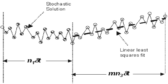
Figure 1: Schematic of the coarse chord slope computation.

The process is illustrated in Fig. 1. In Sections 2 and 3 of this paper we will use this form of chord computation process to perform high-order multistep integration and limit cycles, respectively.

The model problem considered here was chosen (for validation purposes) to be one for which we do know the coarse-grained macroscopic equations - so that comparisons can be made between a coarse stochastic integration based on the microscopic model and the “true” deterministic macroscopic equations for the expected dynamics. We chose one of the examples used in [18]; it is a kinetic Monte Carlo (kMC) realization (using the stochastic simulation algorithm of Gillespie [9, 10]) of a simple surface reaction model for which the mean field evolution equation for the surface coverages ($\theta_{i}$) of the participating species are known [18].

$${{d\theta_{A}}\over{dt}} = \alpha\theta_{*}-\gamma\theta_{A}-4k_{r}\theta_{A}\theta_{B}$$

$${{d\theta_{B}}\over{dt}} = 2\beta\theta_{*}^{2}-4k_{r}\theta_{A}\theta_{B}$$

$${{d\theta_{C}}\over{dt}} = \mu\theta_{*}-\eta\theta_{C}$$ (1)

This is a simplified model of the oxidation of CO ($A$) by dissociatively adsorbing oxygen ($B$) on a Pt catalyst surface in the presence of an additional inert species ($C$). Here $\theta_{*}=1-\theta_{A}-\theta_{B}-\theta_{C}$. For our computations the values of the parameters are set as follows: $\mu=0.36$, $\eta=0.016$, $\alpha=1.6$, $\gamma=0.04$, $k_{r}=1.0$; $\beta$ was set as cited in the text.

The kMC simulations were performed as described in [18] using $N=(1000)^{2}$ adsorption sites and computing the average over several realizations, typically 100. Comparisons were made with numerical integration of the deterministic model eq. (1) using the implicit solver ODESSA [15].

In the next Section we will describe the multi-step coarse projective integration method we use and some preliminary tests that were made to decide on an appropriate order for the projective method. In Section 3 we will discuss the computation of coarse limit cycles through shooting with a coarse projective integrator. In Section 4 we will show how to perform reverse coarse projective integration through forward kMC simulation, and show that the reverse trajectories approach (in negative time) unstable stationary points. We will conclude with a summary and brief discussion.

2 Forward Projective Integration

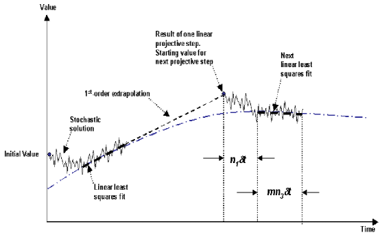
Figure 2: Schematic of first-order coarse projective integration.

Projective integration was introduced in [5]. Its first-order form when used with the estimation of the chord slope from a stochastic integrator is shown in Fig. 2.

In practice we need to use a higher order method. Here we will use an explicit multistep method similar to the Adams-Bashforth method, which can be found in any standard textbook [4]. The third-order method is

$$Y(T+H)=Y(T)+{{H}\over{12}}(23\dot{Y}(T)-16\dot{Y}(T-H)+5\dot{Y}(T-2H))$$

where $H$ is the step size. This formula assumes that we have estimates of the derivatives $\dot{Y}$ that are at least second-order accurate at three places: $T$, $T-H$, and $T-2H$. Higher order methods require correspondingly more derivative estimates of correspondingly higher accuracy ($p$-th order accurate estimates for an order $p+1$ integration method). The formula also assumes that the spacing, $H$, between the integration points is constant. Neither of these assumptions is strictly correct in the stochastic chord slope estimator we are using. Referring to Fig. 1 we see that if the microscopic simulation starts at the point $T$, we will actually estimate the slope of the chord between $T+n_{1}\delta t$ and $T+(n_{1}+mn_{3})\delta t$. This is a first-order accurate estimate of the derivative at $T+(n_{1}+mn_{3}/2)\delta t$, not at $T$. Hence, we need to modify the Adams-Bashforth method in two ways.

To describe the modifications, let us define $T_{n+1}=T_{n}+H$ where $H$ is the “projective step size,” that is, the distance between successive groups of inner steps. Let $T_{n}$ be the center of the chord computed via a least-squares fit. Let $S_{n}$ be the computed slope of that chord. Then we need to integrate from $T_{n}$ to $T_{n}+H-(n_{1}+mn_{3}/2)\delta t$ to get an approximation to the $Y$ value at the start of the next stochastic computation as shown in Fig. 1. This is our first modification to the Adams-Bashforth method. The first order method, which is Euler’s method, is straightforward:

$$Y(T_{n}+H_{0})\approx Y(T_{n})+H_{0}S_{n}$$

where $H_{0}=H-(n_{1}+mn_{3}/2)\delta t$. As long as $S_{n}$ is a zeroth-order accurate approximation to $\dot{Y}(T_{n})$, this is a first-order method. Second and higher-order methods must reflect the fact that the final step is less than the spacing, $H$, between the past points. For example, the second-order method is

$$Y(T_{n}+H_{0})\approx Y(T_{n})+H_{0}(S_{n}+{{H_{0}}\over{2H}}(S_{n}-S_{n-1})).$$

If $S_{n}$ and $S_{n-1}$ are first-order accurate approximations of the derivative, this is a second-order method. Similar modifications apply to higher-order methods, and can be found via routine algebra.

The second modification is due to the fact that we do not compute approximations of the derivatives, but of the slopes of a least-squares linear fit. It is clear that these are first-order approximations to the derivative at the center, so no further adjustment is needed to these integration formulae through second order. However, the order of the difference between $S_{n}$ and $\dot{Y}(T_{n})$ is O($mn_{3}\delta t)$ (ignoring the stochastic noise). The error thereby introduced is of order O($H^{2}(mn_{3}\delta t/H))$. In practice, whether or not an additional correction is needed depends on the size of $mn_{3}\delta t/H$. If it is small, the additional error is unimportant, but if the projective step is not moderately large compared to the length of microscopic integration used to estimate the chord slope, additional corrections to the integration formula are needed if the integration order is higher than two.

Figures 3 and 4 compare the results of projective integration for a trajectory in the vicinity of the periodic oscillations observed at $\beta=20.8$, using $n_{1}\delta t=0.0175$, $mn_{3}\delta t=0.005$, and $H_{0}=0.02$ ($H=0.04$) with an accurate integration using ODESSA. The length of the “settle time”, $n_{1}\delta t$, was based on the size of the fastest time constant corresponding to an eigenvalue around -6. The projective integrator was based on the second-order Adams-Bashforth methods. The order, as well as the projective step size, $H$, were chosen via the comparisons between different order and step sizes shown in Table 1. The values in this table were computed as follows: a point, $(\theta_{A},\theta_{B},\theta_{C})$, in the interior of the attractor in each of the three projected phase-plane plots (as shown in Fig. 4 for the $\theta_{A}-\theta_{B}$ projection) was chosen. Then, the difference between the distances from this point to the “true” limit cycle (as computed by ODESSA) and to the result of a stochastic integration was computed at each integrated output point (or at a sampling of them where they were densely packed). A plot of one such set of errors is shown in Fig. 5. The norm of this error was computed over one limit cycle in each phase plane and the average from the three projected phase planes was used as the error estimate in Table 1.

Projective Step size Euler AB 2nd AB 3rd AB 5th 0.02 0.00025 0.00015 0.00014 0.00017 0.04 0.00102 0.00086 0.00078 unstable 0.06 0.00205 0.00221 0.00301 unstable

Table 1: Average radial deviation from the attractor, for different time-steps and different projective integration methods.

3 Coarse Limit Cycle Computation

When we wish to compute the limit cycle from the output of a coarse time stepper, the main challenges are the noisy nature of the trajectories given by the coarse time-stepper and the fact that the time stepper can only be iterated forward in time.

In order to compute a limit cycle (i.e., write a fixed point algorithm that will converge on the limit cycle), we use the Poincaré map of the trajectory. The Poincaré map is defined by the successive intersections of the time-stepper trajectory with a codimension-1 surface (for this 3D problem we choose conveniently a plane $P(\vec{Y})$) transversal to the flow. For the Poincaré map, a stable periodic trajectory of the original flow becomes an attracting fixed point.

Assuming that $P$ is defined by $\{\vec{Y}\in R^{n}:Y_{j}=C\}$ for the $j-th$ variable, a crossing of the Poincaré plane can be detected when the quantity $(C-Y_{j})$ changes sign [12]. One is only interested in crossings of the surface by the trajectory in the same direction. For noisy systems, care needs to be taken to avoid the detection of false crossings. Uncertainty in any state variable renders the computation of sign changes on such variables unreliable. However, in the presence of sufficient variance reduction, we expect that the ensemble average of many stochastic realizations to be much more reliable, and devise the following procedure to detect a crossing of the Poincaré surface:

1. Monitor the difference $|Y_{j}-C|$ along the trajectory.

2. If $|Y_{j}-C|<\delta$ at some time ($t_{0}$), gather a fixed number of points (M, until $t=t_{0}+M\Delta t$) along the trajectory. With these points, approximate the trajectory of the state variables ($k=1,2,...,n$) via a linear mapping: $Y_{k}=a_{k}t+b_{k}$.

3. Assisted by this local model, confirm that a crossing has occurred. That is, $Y_{j}=C$ for some $t\in[t_{0},t_{0}+M\Delta t]$. If this condition is not met, return to step 1.

Note that this algorithm also gives information about the direction of the crossing (the sign of the slope of the local model for $x_{i}$); thus, the relevant crossings at the Poincaré surface (the ones having the same sign of $a_{i}$) are obtained.

In the neighborhood of a simple stable periodic trajectory, the dynamics on the Poincaré section will appear as a sequence of points approaching the fixed point. Implementing a Newton-Raphson-type contraction mapping on the coarse return map, the convergence to the fixed point of the sequence (i.e., to the periodic trajectory of the flow) can be accelerated. This contraction map is defined as follows. Let x be the vector of components of $Y$ excluding $Y_{i}$ used to define the Poincaré section.

$${\bf x}^{k+1}={\bf x}^{k}=-J({\bf x}^{k})^{-1}({\bf x}^{k}-{\bf x}^{k-1})$$

where $J$ is the Jacobian of the linearization of the Poincaré map (corresponding to the monodromy matrix for the limit cycle).

The Jacobian can be estimated by applying perturbations around the current Poincaré crossing. A “centered difference” ensemble of perturbations are used to estimate numerical derivatives, which are naturally sensitive to noise. For problems with many coarse variables, Newton-Krylov type methods based on coarse timesteppers are being explored (such as the Recursive Projection Method of Shroff and Keller, or Newton-Picard methods [24, 17]); the sensitivity of these matrix-free methods to noise is an important focus of current research.

3.1 Results

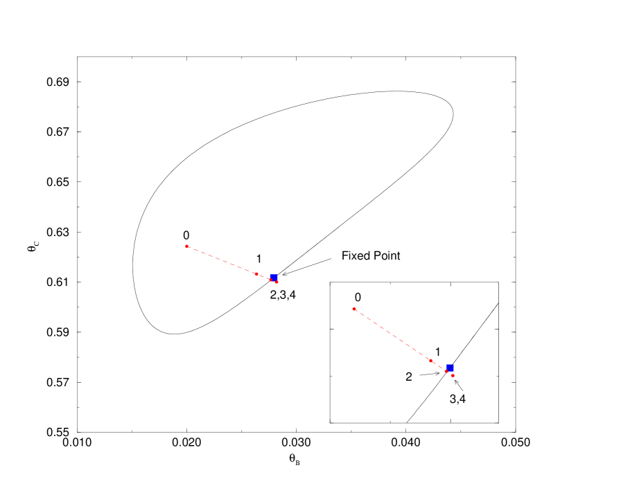
Figure 6: Fixed point iteration and convergence to the coarse limit cycle with $\beta=20.24$. The initial point is marked 0, remaining points are given by a coarse Newton-type iteration formula.

The kMC simulations were performed as described in Section 2 using $N=(1000)^{2}$ adsorption sites and computing the average over 100 realizations for $\beta=20.24$ . The deterministic (mean-field approximation) system exhibits, at these conditions, a single, attracting periodic trajectory. Observing on a Poincaré map defined by the plane $\theta_{A}=0.33$ and considering only crossings with negative slope, the fixed point of the Poincaré section is found at $(\theta_{B},\theta_{c})=(0.027947,0.61173)$. It is indicated with a filled square in Fig. 6. In addition to the ubiquitous Floquet multiplier at 1, the leading multiplier is 0.72147 while the second multiplier is $2.92\times 10^{-8}$. The return time is 183.89 time units. For the selected value of $\beta$, trajectories converge very slowly on the limit cycle.

3.1.1 Converging to the Limit cycle

Note the drastic time-scale separation implied by the orders of magnitude difference of the Floquet multipliers of the deterministic, mean field limit cycle. This suggests that perturbations along one direction of the two-dimensional Poincaré section decay very quickly. In order to avoid large numerical sensitivity during the Jacobian estimation, we exploit this separation of time scales by resorting to an effectively one-dimensional approach. In the time interval of even a single return time, we can consider that $\theta_{C}$ at the Poincaré crossing becomes slaved to $\theta_{B}$. This fast slaving is “embodied” in the eigenvector of the fast (strongly stable) Floquet multiplier (we can “read” it in the corresponding eigenvector of the linearization around the fixed point for the deterministic – mean-field – system). The resulting line equation (see Fig. 6 all points of the NR iteration lie on it) is:

$$\theta_{C}=(1.0-2.63149316\theta_{B})/1.51747895$$

Performing the contraction mapping computations in the remaining one dimension converges to the coarse fixed point with an an error $O(10^{-4})$, commensurate with the expected uncertainty level from the kMC simulation. Our convergence criterion (maximum deviation) was set to 0.0001 on the coarse iteration variable $\theta_{B}$. Our contraction mapping converges after 4 iterations (point 0 on Fig. 6 is the initial point). The derivatives of the map were estimated using three perturbations around the current point and fitting a least-squares line (3 points); the perturbations were 0.0005, 0.0, and -0.0005 on $\theta_{B}$. The estimated coarse leading multiplier was 0.7274 and the coarse return time 188.19 time units; the location of the coarse fixed point is estimated to be at $(0.0282,0.6101)$, all in good agreement with the mean-field approximation.

4 Reverse Projective Integration

Reverse projective integration, described in [6], is a version of projective integration in which the inner integrator proceeds in the forward direction while the projective step is taken in the reverse direction. It was used in [6] because of its unusual stability properties that enabled us to find certain classes of stationary points. Here we use it to integrate backward in time when the microscopic system can only be evolved forward in time, either because of its nature or because it is defined by a legacy code which cannot easily be modified.

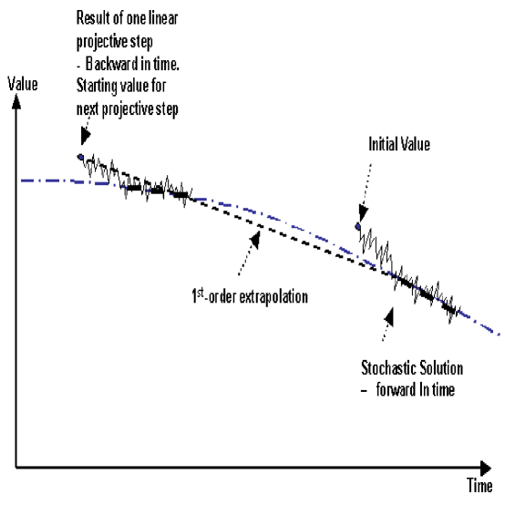
Figure 7: Schematic of reverse coarse projective integration.

Reverse integration is illustrated in Fig. 7 with a linear projective step. In [6] it was shown that reverse projective integration damps components corresponding to large negative eigenvalues - components that would be unstable in normal reverse integration were the latter possible. The reverse projective step causes the method to also be damping for components corresponding to small positive eigenvalues since these decay in reverse time. Thus reverse projective integration allows us to approach stationary points that are stable or unstable (including saddle points), provided that the local eigenvalues in the negative half plane have large negative real parts while any in the positive half plane have small real parts.

When the microscopic model is stochastic, it is usually inherently uni-directional in time. For example, a random walk will give rise to effective diffusion, even if the sign of all movements (and thus, time) was reversed. This has been exploited in [13] to guide molecular dynamics simulations backwards on a free energy surface, and in the location of transition states. Here, we will combine a stochastic microscopic model with a reverse projective integrator to approach, backward in time, a stationary saddle point of a KMC model.

Note that many types of fixed points can be located performing contraction mappings “wrapped around” the coarse timestepper (e.g. the Shroff and Keller RPM [24]). That procedure, however, requires a good initial condition. Reverse integration gives approximations to backward in time trajectories that will be attracted (in reverse time) to these forwardly unstable points.

To illustrate this method we first use a further simplification of eq. (1) to a single ODE that has an unstable stationary point (its sole eigenvalue is positive). It is given in [18] as

$${{d\theta}\over{dt}}=\alpha(1-\theta)-\gamma\theta-k_{r}(1-\theta)^{2}\theta$$ (2)

where now, $\alpha=1.0$, and $\gamma=0.01$. In this case, eq. (2) can be integrated in reverse time to find the unstable stationary point. Reverse projective integration can also be used to find that stationary point. Fig. 8 shows the comparison between the reverse deterministic and reverse projective-stochastic integrations for a particular initial condition. The parameter $k_{r}$ was set to 5. The trajectories (starting at time=0.0) approach the unstable fixed point at $\theta=0.7357$ whose eigenvalue is about 0.58. The deterministic trajectory was obtained from ODESSA [15] with a reporting horizon of -0.02 units and a tolerance of $1\times 10^{-9}$. The reverse projective method used the stochastic code forward for 0.02 units of time and then the Adams-Bashforth second-order formula, as described above, with a time step of -0.12 time units. As before, we used for this example $10^{6}$ adsorption sites and the results are averaged over 100 simultaneous realizations.

Figure  9 shows similar integrations for the “full” version, eq. (1). The parameter $\beta$ is set to 20.8. The reverse trajectories approach a saddle stationary point in reverse time. The eigenvalues of the linearization of the flow along the deterministic trajectory are presented in Fig. 10(a) and (b). In this case, the deterministic trajectory was also calculated using reverse projective integration with ODESSA as the inner integrator in the forward direction. (This was necessary because of the saddle nature of the stationary point, meaning that direct reverse integration would be unstable and explode backward in time.) ODESSA was used to integrate for one unit of time in the forward direction and then a projective Adams-Bashforth step was used in the reverse direction for two units of time. We confirmed, by starting at the “end” of the reverse trajectory, and using ODESSA normally forward in time, that the reverse projective trajectory was indeed traced by the code in forward time Fig. 12. The projective stochastic solution was calculated with the same steps, but the forward evolution was carried out with the stochastic code. Significant numerical noise arises along the stochastic trajectory. This noise can be partially explained by studying the linearization of the vectorfield (computed or estimated) along the trajectory and in particular the eigenvalues closer to zero. A small perturbation along the trajectory is amplified by the factors plotted in Fig. 10(c) (these are $e^{\lambda\delta t}$ for the largest $\lambda$, where $\delta t$ is the total reverse integration time step). Even when such perturbations (that are a natural part of the stochastic simulation results) are not amplified, they decay very slowly. The choice of time-step is critical, as we need to use a relatively long forward “inner” integration to damp the stiff eigencomponents which would otherwise blow up the backward trajectory. Fig. 9(b) and (c) shows that the deterministic and the stochastic reverse projective trajectories are similar when plotted in phase-space.

Figure 11 shows the same results when the reverse trajectory is initiated closer to the saddle point, beyond the region where perturbations are amplified (at the point of the deterministic trajectory of Fig. 9 where time=-180 s). The agreement is better, although still not noise-free. The important point is that the reverse trajectory asymptotically tends to the saddle point.

5 Conclusion

We have demonstrated the use of projective integration techniques for simulating the coarse dynamic behavior of models described by microscopic models. In this paper, the “inner” microscopic model was a kinetic Monte Carlo simulation of surface reaction schemes based on the Stochastic Simulation Algorithm of Gillespie. It is worth noting more recent work by Gillespie on the so-called “tau-leaping” method, which can be used under some circumstances to accelerate stochastic simulation algorithms (SSAs) [11]. Our coarse projective integration schemes are computational “wrappers” around “inner evolution” schemes; as such, they can be wrapped around a “tau-leaping” inner SSA. Implicit versions of coarse projective integrators have been introduced in [5]; studying the analogies and differences between these methods and the “implicit tau-leaping” schemes of Rathinam et al. [22] is a subject of current research.

Beyond the illustration of coarse projective integration in a kinetic Monte Carlo context, the focus of this paper was in the use of such schemes to perform tasks beyond direct simulation. Reverse coarse projective integration was demonstrated; its ability, under certain circumstances, to approach unstable, saddle-like objects in coarse phase space may prove helpful in the location of transition states in computational chemistry (see the coarse MD example in [13]). We also illustrated the use of projective integration in the solution of coarse boundary value problems, in particular the location and computer-assisted stability analysis of coarse limit cycles for the expected behavior of the microscopic simulator.

Remarkably, these algorithms have counterparts in the case of continuum numerical analysis also; these counterparts are particularly meaningful in the context of accelerating legacy simulators for continuum problems (see for example the stability analysis in [5] and [6]). They also constitute the inspiration for further algorithms, like telescopic projective integrators [5] for problems with several gaps in their eigenvalue spectrum, as well as coarse Langevin-based acceleration techniques for problems whose dynamics are governed by rare events. The extraction of macroscopic dynamics from microscopic/stochastic simulators constitutes the current frontier in multiscale/complex system computation [8]. Equation-free techniques, based on coarse time-stepping, aim at solving these macroscopic equations without ever deriving them in closed form; as such, techniques like the coarse projective integration illustrated here constitute a bridge between traditional continuum numerical analysis and detailed physical modeling of complex systems.

Acknowledgements This work was partially supported by AFOSR (Dynamics and Control), an NSF-ITR grant (IGK, CWG) and Fulbright- García Robles and CONACYT Fellowships (RRM). Discussions with Profs. Li Ju, P. G. Kevrekidis, L. Petzold and Dr. G. Hummer are gratefully acknowledged.

Figure 3: An illustration of forward coarse projective integration. Periodic trajectory of the model system computed using the mean-field equations (solid line), and the kMC simulator (dashed line). A second-order Adams-Bashforth integrator was used to compute the kMC trajectory with $n_{1}\delta t=0.0175$, $mn_{3}\delta t=0.005$, and $H_{0}=0.02$ ($H=0.04$) for the projective algorithm. For this example $\beta=20.8$, other parameters of the model were set as indicated in the text.

Figure 4: Attractor comparison in the $\theta_{A}-\theta_{B}$ projection for the results presented in Fig. 3.

Figure 5: Local errors (angle parametrization, around the point (0.22,0.07,0.7)) for the $\theta_{A}-\theta_{B}$ phase plane projection of the attractor. Results of several integrator orders using the example illustrated in Fig. 3 are presented.

Figure 8: Backward projective integration for the simplified model. The trajectory approaches an unstable fixed point.

Figure 9: Backward integration for the full model with $\beta=20.8$. (a) Time-series of $\theta_{A}$ evolution, (b) and (c) Projections of the trajectory in phase-space. The parameters of the projective integrator, and other parameters of the model, are described in the text.

Figure 10: Backward integration for the full model. (a) and (b) eigenvalues along the trajectory. (c) amplification factor for perturbations at various locations along the trajectory.

Figure 11: Backward integration for the full model. (a) Time-series of $\theta_{A}$ evolution, (b) and (c) Projections of the trajectory in phase-space.

Figure 12: Comparison of backward and forward integration for the example in Fig. 9. The forward integration trajectory (dashed line) was obtained by using, as a starting point, the final point of the backward integration.

References

- [1] Chorin, A. J., Kast, A. and Kupferman, R., Optimal prediction of underresolved dynamics, Proc. Nat. Acad. Sci. USA, 95:4094-4098 (1998).
- [2] Chorin, A. J., Hald, O. H. and Kupferman, R., Optimal prediction and the Mori-Zwanzig representation of irreversible processes, Proc. Nat. Acad. Sci. USA, 97:2968-2973 (2000).
- [3] Constantin, P., Foias, C., Nicolaenko, B. and Temam, R., Integral Manifolds and Inertial Manifolds for Dissipative Partial Differential Equations, Springer Verlag, NY (1988).
- [4] Gear, C. W., Numerical Initial Value Problems in Ordinary Differential Equations, Prentice Hall, Englewood Cliffs, NJ, 1971.
- [5] Gear, C. W. and Kevrekidis, I. G, Projective Methods for Stiff Differential Equations: Problems with gaps in their eigenvalue spectrum, SIAM J. Sci. Comput., 24:1091–1106 (2003).
- [6] Gear, C. W. and Kevrekidis, I. G, Computing Stationary Points of Unstable Stiff Systems, unpublished. Can be obtained at nlin.CD/0302055 at arXiv.org.
- [7] Gear, C. W., Kevrekidis, I. G and Theodoropoulos, C., “Coarse” integration/bifurcation analysis via microscopic simulators: Micro-Galerkin methods, Comput. Chem. Eng., 26:941–963 (2002).
- [8] Givon, D., Kupferman, R. and Stuart, A., Extracting Macroscopic Dynamics: model problems and algorithms. University of Warwick, Preprint 11/2003.
- [9] Gillespie, D.T., General method for numerically simulating stochastic time evolution of coupled chemical-reactions, J. Comput. Phys., 22:403–434 (1976).
- [10] Gillespie, D.T., Exact stochastic simulation of coupled chemical reactions, J. Phys. Chem., 81:2340–2361 (1977).
- [11] Gillespie, D.T., Approximate accelerated stochastic simulation of chemically reacting systems, J. Chem. Chem., 115:1716–1733 (2001).
- [12] Hénon, M., On the numerical computation of Poincaré maps, Physica D, 5:412-414 (1982).
- [13] Hummer, G. and Kevrekidis, I. G, Coarse molecular dynamics of a peptide fragment: Free energy, kinetics, and long-time dynamics computations, J. Chem. Phys., 118:10762–10773 (2003).
- [14] Kevrekidis, I. G., Gear, C. W., Hyman, J. M., Kevrekidis, P. G., Runborg, O. and Theodoropoulos, K., Equation-free multiscale computation: enabling microscopic simulators to perform system-level tasks, Submitted to Comm. Math. Sciences. (also NEC Technical Report, NEC-TR 2002-010N, http://www.neci.nj.nec.com/homepages/cwg/), August 2002.
- [15] Leis, J. R. and Kramer M. A., ODESSA – An ordinary differential equation solver with explicit simultaneous sensitivity analysis, ACM Trans. Math. Software, 14:61–67 (1988).
- [16] Li, J., Kevrekidis, P.G., Gear, C.W. and Kevrekidis, I.G., Deciding the nature of the coarse equation through microscopic simulations: The baby-bathwater scheme, Multiscale Model. Simul., in press (2003).
- [17] Lust, K., Roose, D., Spence, S. and Champneys, A. R., An adaptive Newton-Picard algorithm with subspace iteration for computing periodic solutions, SIAM J. Sci. Comput., 19:1188–1209 (1998).
- [18] Makeev, A. G., Maroudas D. and Kevrekidis, I.G., “Coarse” stability and bifurcation analysis using stochastic simulators: Kinetic Monte Carlo Examples, J. Chem. Phys., 116:10083–10091 (2002).
- [19] Makeev, A.G., Maroudas, D., Panagiotopoulos, A. Z. and Kevrekidis, I.G., Coarse bifurcation analysis of Kinetic Monte Carlo Simulations: A lattice-gas model with lateral interactions, J. Chem. Phys., 117:8229–8240 (2002).
- [20] Melchior, M. and Oettinger, H.C., Variance reduced simulations of polymer dynamics, J. Chem. Phys., 105:3316–3331 (1996).
- [21] Melchior, M. and Oettinger, H.C., Variance reduced simulations of stochastic differential equations, J. Chem. Phys., 103:9506–9509 (1995).
- [22] Rathinam, M., Petzold, L. R., Cao, Y. and Gillespie, D.T., Stiffness in stochastic chemically reacting systems: The implicit Tau-leaping method, preprint, University of Maryland Baltimore County, Department of Mathematics and Statistics (2003).
- [23] Runborg, O., Theodoropoulos, C. and Kevrekidis, I. G., Effective bifurcation analysis: A time-stepper-based approach, Nonlinearity, 15:491-511 (2002).
- [24] Shroff, G.M. and Keller, H. B., Stabilization of unstable procedures– The recursive projection method, SIAM J. Numer. Anal., 30:1099–1120 (1993).
- [25] Siettos, C. I., Armaou, A., Makeev, A. G. and Kevrekidis, I. G., Microscopic/Stochastic timesteppers and Coarse Control: A kinetic Monte Carlo example, AIChE J., in press (2003).
- [26] Siettos, C. I., Graham, M. D. and Kevrekidis, I. G., Coarse Brownian dynamics for nematic liquid crystals: Bifurcation, projective integration, and control via stochastic simulation, J. Chem. Phys., 118:10149–10156 (2003).
- [27] Temam, R., Infinite Dimensional Dynamical Systems in Mechanics and Physics Springer Verlag, NY (1988).
- [28] Theodoropoulos, C., Qian, Y. H. and Kevrekidis, I. G., Coarse stability and bifurcation analysis using time-steppers: A reaction-diffusion example, PNAS, 97:9840–9843 (2000).
- [29] Theodoropoulos, K., Sankaranarayanan, S., Sundaresan, S. and Kevrekidis, I. G., Coarse bifurcation studies of bubble flow microscopic simulations, Chem. Eng. Sci., in press (2003). Can also be obtained at nlin.PS/0111040 at arXiv.org.