Asymptotic Behavior of a Model of Characteristic Earthquakes and its Implications for Regional Seismicity

Abstract

The recently introduced Minimalist Model [Vázquez-Prada et al, 2002] of characteristic earthquakes provides a simple representation of the seismicity originated in a single fault. Here, we first characterize the properties of this model for large systems. Then, assuming, as it has been observed, that the size of the faults in a big enough region is fractally distributed, with a fractal dimension $D=1.7$, we describe the total seismicity produced in that region. The resulting catalogue accounts for the addition of all the characteristic events triggered in the faults and also includes the rest of non-characteristic earthquakes. The global accumulated size-frequency relation correctly describes a Gutenberg-Richter form, with a $b$ exponent of around 0.7.

LÓPEZ-RUIZ ET AL. A MODEL OF CHARACTERISTIC EARTHQUAKES J. B. Gómez, Departmento de Ciencias de la Tierra, Universidad de Zaragoza, Pedro Cerbuna 12, Facultad de Ciencias, Edificio C, 50009 Zaragoza, España. (jgomez@unizar.es)

1 Introduction

In regional and global seismicity, there is a well established fractal relation, the Gutenberg-Richter law, that can be expressed in the form

$$\dot{N}\propto S^{-b},$$ (1)

where $\dot{N}$ is the number of observed earthquakes in a year with rupture area greater than $S$, and $b$ is the so-called $b$-value, which is in the range 0.5-1.5. The Gutenberg-Richter law implies that earthquakes are, on a regional or global scale, a self-similar phenomenon without any characteristic length scale.

It is important to notice, however, that the Gutenberg-Richter law is a property of regional seismicity, appearing when we average seismicity over big enough areas and long enough time intervals. In the last ten years, a wealth of data has been collected to extract statistics on individual systems of earthquake faults [Wesnousky, 1994; Sieh, 1996; Petersen et al., 1996]. Interestingly, it has been found that the distribution of earthquake magnitudes may vary substantially from one fault to another and that, in general, this type of size-frequency relationship is different from the Gutenberg-Richter law. Many single faults or fault zones display power-law distributions only for small events (small compared with the maximum earthquake size a fault can support, given its area), which occur in the intervals between roughly quasi-periodic earthquakes of much larger size which rupture the entire fault. These large quasi-periodic earthquakes are termed “characteristic” [Schwartz and Coppersmith 1984], and the resulting size-frequency relationship, Characteristic Earthquake distribution.

With the purpose of representing the seismicity originated in a single fault, we have recently introduced a simple model called “Minimalist” [Vázquez-Prada et al, 2002]. In this model, a one-dimensional vertical array of length $N$ is considered. The ordered levels of the array are labelled by an integer index $i$ that runs upwards from 1 to $N$. This system performs two basic functions: it is loaded by receiving stress particles in its various levels and unloaded by emitting groups of particles through the first level $i=1$. These emissions which relax the system are considered to be earthquakes, and the number of consecutively empty lower levels, $k$, in each event is assumed to be equal to the ruptured area.

The main goal of this paper is the study of the total seismicity produced in a region, using the Minimalist Model for the description of the seismicity coming from each individual fault. Thus in the coming paragraphs, we will briefly review some properties of the Minimalist Model, and will identify its asymptotic ($N\rightarrow\infty$) behavior. This information, crossed with the observed fractal distribution of fault sizes at a regional level, will give us a size-frequency distribution for the earthquake population which will be discussed and compared with Eq. (1).

2 The Minimalist Model and its Asymptotic Behavior

In the Minimalist Model, the rules for the loading and relaxing functions in the system are:

1. The incoming particles arrive at the system at a constant time rate. Thus, the time interval between each two successive particles will be considered the basic time unit in the evolution of the system.

2. All the positions in the array, from $i=1$ to $i=N$, have the same probability of receiving a new particle. When a position receives a particle we say that it is occupied.

3. If a new particle comes to a level which is already occupied, this particle has no effect on the system. Thus, a given position $i$ can only be either non-occupied when no particle has reached it, or occupied when one or more particles have.

4. The level $i=1$ is special. When a particle goes to this first position a relaxation event occurs. Then, if all the successive levels from $i=1$ up to $i=k$ are occupied, and position $k+1$ is empty, the effect of the relaxation –or earthquake– is to unload all the levels from $i=1$ up to $i=k$. Hence, the size of this relaxation is $k$, and the remaining levels $i>k$ remain unaltered in their occupancy.

Thus, we notice that this model was devised in a spirit akin to the Sand-Pile model of Self- Organized Criticality: physics is not apparent, but the model is able to grasp the basics of the routine of a fault dynamics. In this case, the presence of an asperity controlling the mechanism of relaxation in the system, is a necessary ingredient of this cellular automaton.

From what has been mentioned above, this model has no parameter; the size $N$ is the unique specification to be made, and the spatial correlation is induced by rule 4 above. Now, the state of the system is given by stating which of the ($i>1$) $N-1$ levels are occupied. Each of these states corresponds to a stable configuration, and therefore the total number of possible configurations is $2^{(N-1)}$. We use the term “total occupancy” for the configuration in which all levels except the first are occupied.

As this model is one-dimensional, extensive Monte Carlo simulations can be performed to accurately explore its properties. It can also be studied, for small system sizes, from the perspective of Markov Chains [Vázquez-Prada et al, 2002].

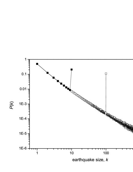
Figure 1: Probability of occurrence of earthquakes of size $k$ in the Minimalist Model. Three simulations are superimposed, corresponding to systems with $N=10$, $N=100$, and $N=1000$ elements.

The results for the earthquake size-frequency relation, $p_{k}$, are drawn in Figure 1. In this figure, there are two notable properties to be commented on. First and most important, we see that the characteristic relaxation, $k=N$, has a much higher probability of occurrence than the big relaxations but with $k<N$. In fact, for $N=10$, $100$ and $1000$, the probability of these three characteristic relaxations differs very little, and is about $10\%$. We can express this fact by saying that in this model, grosso modo, one would likely observe only very small earthquakes and the characteristic one. And secondly, we observe the perfect coincidence of these curves of probability for systems of different size $N$.

This second property of the model is related to what we will call henceforth the “tail splitting” property , which is expressed by the relation

$$P_{N}(N)=P_{N+1}(N+1)+p_{N}(N+1).$$ (2)

The meaning of this expression is as follows. The probability of occurrence of a characteristic earthquake in a system of size $N$ is equal to the sum of the probability of a characteristic in a system of size $N+1$ plus the probability of a non-characteristic of size $N$ in a system of size $N+1$. Thus, capital letter $P$ is reserved for the probability of a characteristic event, and small $p$ for the probability of non-characteristic earthquakes, which are independent of the system size.

This “tail splitting” property holds in a family of models that include the Minimalist Model. Its consequence is that if one knows $p_{k}(N)$ for all $1\leq k<N$, then one knows $P_{M}(M)$ for $1\leq M\leq N$. And vice versa, using Eq. (2), the knowledge of the $P$s leads to the knowledge of the $p$s. In the Minimalist Model, the value of these two sets of probabilities can be easily obtained, for small $N$, by means of diagonalizations of the corresponding Markov matrices, and in general by Montecarlo simulations. For large systems one expects a regular behavior in the decaying rate of these probabilities. This information is shown in Fig. 2. In Fig. 2a, the values of the $P$s are fit by the function

$$P_{N}(N)=c(\log N)^{-\alpha},$$ (3)

where $\alpha=0.95$ and $c$ is a constant. Eq. (3) means that the probability of occurrence of a characteristic earthquake goes to zero as the system size goes to infinity, although very slowly. For example, for a system of size $N=1000$ the probability of a characteristic earthquake is $P_{1000}(1000)=0.07582$; for a system size $N=10^{6}$, $P_{10^{6}}(10^{6})=0.04662$; and for a system size $N=10^{8}$, $P_{10^{8}}(10^{8})=0.02986$. A difference of five orders of magnitude in system size produces a drop in the probability of a characteristic earthquake from 7.5% to 3%. Equating the rupture area of an earthquake with the parameter $N$ in the minimalist model, a difference of five orders of magnitude in rupture area is roughly that which exists between earthquakes of magnitude 3 and 8.

As a verification of the goodness of this fit, in Fig. 2b we have plotted the ratio $P_{N}(N)/P_{N^{\prime}}(N^{\prime})$ of the probability of a characteristic earthquake for two different system sizes ($N$ and $N^{\prime}$) against the ratio $(\log N^{\prime}/\log N)^{\alpha}$ for $\alpha=0.95$. If Eq. (3) does indeed describe well the asymptotic behavior of the probability of occurrence of characteristic earthquakes in the minimalist model, then this plot should be a straight line of slope 1. The points are colour-coded with respect to the offset between the values of $N$ and $N^{\prime}$ used to calculate the ratios $P_{N}(N)/P_{N^{\prime}}(N^{\prime})$ and $(\log N^{\prime}/\log N)^{\alpha}$. An offset of one means that the ratio is calculated for two consecutive data points. An offset of two is for ratios calculated for next-nearest neighbor data points, and so on. As can be seen, all the data points, regardless of the offset, fall on the slope-one straight line, indicating that function (1) is a good description of the asymptotic behavior. To further check that the value $\alpha=0.95$ is statistically different from $\alpha=1$, in Fig. 2c we have plotted again the same ratios as in Fig. 2b but with an exponent $\alpha=1$. The clear departure from the slope-one straight line for big offsets shows that the correct exponent is $\alpha=0.95$ and not $\alpha=1$.

Now, using Eqs. (2) and (3), always for large $N$, we have

$$c(\log N)^{-\alpha}=c(\log(N+1))^{-\alpha}+p_{N}(N+1)$$ (4)

and therefore

$$p_{N}(N+1)=\frac{c\alpha}{N(\log N)^{\alpha+1}}.$$ (5)

3 Implication for the global seismicity and discussion

Observational data seem to show that the frequency-size distribution of faults is fractal [Hirata, 1989, Barton et al., 1996]. Specifically, the results of Barton et al. (1995) in Nevada indicate that the fractal dimension has a mean value of $D=1.7$. Using this information, our result for the probability of occurrence of an earthquake of size $k$ originated in any of the faults of the region is

$$p_{k}\approx\sum^{\infty}_{N=k+1}N^{-D}\frac{c\alpha}{k(\log k)^{\alpha+1}}+k^{-D}\frac{c}{(\log k)^{\alpha}}.$$ (6)

In this formula, the first term accounts for the contribution of the non-characteristic earthquakes originated in the faults, and the second corresponds to the contribution of only the characteristic ones. Eq. (6) is equivalent to

$$p_{k}\approx\frac{c\alpha}{k(\log k)^{\alpha+1}}\sum^{\infty}_{N=k+1}N^{-D}+k^{-D}\frac{c}{(\log k)^{\alpha}}.$$ (7)

After computing the sum in the first term, we obtain

$$p_{k}\approx\frac{c\alpha}{k(\log k)^{\alpha+1}}\frac{k^{1-D}}{D-1}+k^{-D}\frac{c}{(\log k)^{\alpha}}.$$ (8)

Rearranging this equation, we get

$$p_{k}\approx k^{-D}\frac{c}{(\log k)^{\alpha}}\left(1+\frac{\alpha}{D-1}\frac{1}{\log k}\right).$$ (9)

When $k$ is large, Eq. (9) simplifies to

$$p_{k}\propto k^{-D}\frac{1}{(\log k)^{\alpha}}.$$ (10)

In other words, the net result is equivalent to the product of a first factor coming from the fault size distribution times a second factor coming from the seismicity of the individual faults. Note that the impact of the second factor, i.e. the logarithmic term, in the decay rate of $p_{k}$, is very light in comparison to the first power-law factor coming from the assumed fault distribution. This is put in evidence in Fig. 3a, where simulating the regional seismicity, we have drawn all the earthquakes resulting from a large number of minimalist systems, acting simultaneously, and distributed in size in the fractal form $N^{-D}$ with $D=1.7$. In Fig.3b, we have reorganized the information of Fig.3a, in an accumulated distribution for a more direct comparison with Eq. (1). As shown in this figure, our result corresponds to a Gutenberg-Richter relation with an exponent around 0.75.

Hence, our main conclusion in this paper is that, using this model, the slope $b$ appearing in the Gutenberg-Richter graph of the regional seismicity is basically due to the effect of the fractal distribution of fault sizes.

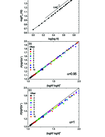
Figure 2: Asymptotic behavior of the Minimalist Model. (a) Logarithmic-decaying fit to the probability of occurrence of the characteristic earthquake in a system of size $N$. (b) Plot of the ratio $P_{N}(N)/P_{N^{\prime}}(N^{\prime})$ against the ratio $(\log N^{\prime}/\log N)^{\alpha}$, for $\alpha=0.95$, where $N$ and $N^{\prime}$ are two different system sizes. If the logarithmic-decaying fit is correct, all the data points in this graph should plot on the diagonal straight line of slope one, as is the case. (c) Same as (b), but with $\alpha=1$ to show that the value $\alpha=0.95$ is statistically different from $\alpha=1$. In this case the large-offset data points plot off the slope one line.

Figure 3: (a) Discrete Gutenberg-Richter relation for earthquakes occurring in minimalist-model faults with a power-law (fractal) size-frequency distribution with fractal dimension $D=1.7$. The slope of the straight line is $-1.78$. (b) Accumulated Gutenberg-Richter relation for earthquakes occurring in minimalist model faults with a power-law (fractal) size-frequency distribution. The slope of the straight line is $-0.75$.

- [1] Barton, Ch.C., Cameron, B.G., and Montgomery, J.R., Fractal scaling of fracture and fault maps at Yucca Mountain, Southwestern Nevada, EOS, 67 (44), 871, 1986.
- [2] Hirata, T., Fractal dimension of fault systems in Japan: fractal structure in rock fracture geometry at various scales, PAGEOPH, 131, 157-170, 1989.
- [3] Petersen, M. D., Bryant, W. A., Cramer, C. H.; Cao, T., Reichle, M., Frankel, A. D., Lienkaemper, J. J., McCrory, P. A., and Schwartz, D. P.: Probabilistic Seismic Hazard Assessment for the State of California. California Department of Conservation s Division of Mines and Geology Open-File Report 96-08, and United States Geological Survey Open- File Report 96-706, 66 pp., 1996.
- [4] Schwartz, D.P., and Coppersmith, K.J., Fault behavior and characteristic earthquakes: Examples from the Wasatch and San Andreas fault zones J. Geophys. Res., 89, 5681, 1984.
- [5] Sieh, K., The repetition of large-earthquake ruptures Proc. Natl. Acad. Sci. USA, 93, 3764-3771, 1996.
- [6] Vazquez-Prada, M., González, A. Gómez, J.B., and Pacheco, A.F., A Minimalist Model of Characteristic Earthquakes, Nonlin. Proc. Geophys., 9(4), 513-519, 2002.
- [7] Wesnousky, S.G., The Gutenberg-Richter or Characteristic Earthquake Distribution, Which is it? Bull. Seismol. Soc. Am, 84, 1940-1959, 1994.