Abstract

In this chapter, I review the main methods and techniques of complex systems science. As a first step, I distinguish among the broad patterns which recur across complex systems, the topics complex systems science commonly studies, the tools employed, and the foundational science of complex systems. The focus of this chapter is overwhelmingly on the third heading, that of tools. These in turn divide, roughly, into tools for analyzing data, tools for constructing and evaluating models, and tools for measuring complexity. I discuss the principles of statistical learning and model selection; time series analysis; cellular automata; agent-based models; the evaluation of complex-systems models; information theory; and ways of measuring complexity. Throughout, I give only rough outlines of techniques, so that readers, confronted with new problems, will have a sense of which ones might be suitable, and which ones definitely are not.

[Overview of Methods and Techniques]Methods and Techniques of Complex Systems Science: An Overview

1 Introduction

A complex system, roughly speaking, is one with many parts, whose behaviors are both highly variable and strongly dependent on the behavior of the other parts. Clearly, this includes a large fraction of the universe! Nonetheless, it is not vacuously all-embracing: it excludes both systems whose parts just cannot do very much, and those whose parts are really independent of each other. “Complex systems science” is the field whose ambition is to understand complex systems. Of course, this is a broad endeavor, overlapping with many even larger, better-established scientific fields. Having been asked by the editors to describe its methods and techniques, I begin by explaining what I feel does not fall within my charge, as indicated by Figure 1.

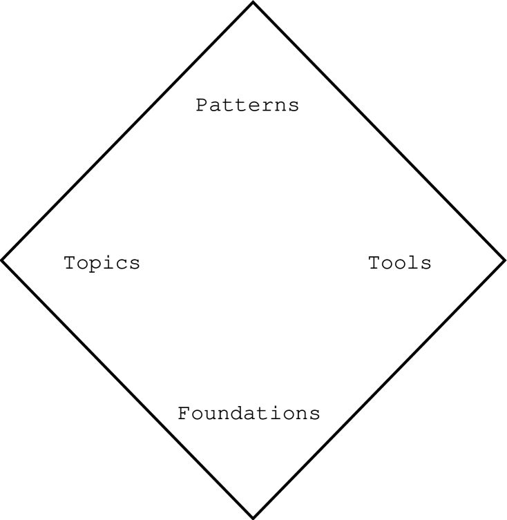
Figure 1: The quadrangle of complex systems. See text.

At the top of Figure 1 I have put “patterns”. By this I mean more or less what people in software engineering do [Design-Patterns-gang-of-four]: a pattern is a recurring theme in the analysis of many different systems, a cross-systemic regularity. For instance: bacterial chemotaxis can be thought of as a way of resolving the tension between the exploitation of known resources, and costly exploration for new, potentially more valuable, resources (Figure 2). This same tension is present in a vast range of adaptive systems. Whether the exploration-exploitation trade-off arises among artificial agents, human decision-makers or colonial organisms, many of the issues are the same as in chemotaxis, and solutions and methods of investigation that apply in one case can profitably be tried in another [Anderson-random-walk-learning, Mueller-et-al-optimization-via-chemotaxis]. The pattern “trade-off between exploitation and exploration” thus serves to orient us to broad features of novel situations. There are many other such patterns in complex systems science: “stability through hierarchically structured interactions” [Simon-architecture], “positive feedback leading to highly skewed outcomes” [Simon-skew], “local inhibition and long-rate activation create spatial patterns” [Turing-morphogenesis], and so forth.

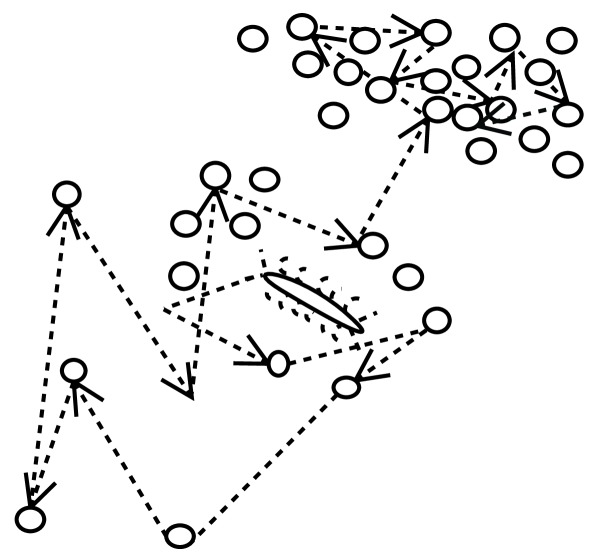
Figure 2: Bacterial chemotaxis. Should the bacterium (center) exploit the currently-available patch of food, or explore, in hopes of finding richer patches elsewhere (e.g. at right)? Many species solve this problem by performing a random walk (jagged line), tumbling randomly every so often. The frequency of tumbling increases when the concentration of nutrients is high, making the bacterium take long steps in resource-poor regions, and persist in resource-rich ones [Strong-et-al-optimal-chemotaxis, Alon-et-al-robustness-of-chemotaxis, Yi-et-al-perfect-adaptation-in-chemotaxis].

At the bottom of the quadrangle is “foundations”, meaning attempts to build a basic, mathematical science concerned with such topics as the measurement of complexity [Badii-Politi], the nature of organization [Fontana-Buss-organization], the relationship between physical processes and information and computation [complexity-entropy-physics-of-info] and the origins of complexity in nature and its increase (or decrease) over time. There is dispute whether such a science is possible, if so whether it would be profitable. I think it is both possible and useful, but most of what has been done in this area is very far from being applicable to biomedical research. Accordingly, I shall pass it over, with the exception of a brief discussion of some work on measuring complexity and organization which is especially closely tied to data analysis.

“Topics” go in the left-hand corner. Here are what one might call the “canonical complex systems”, the particular systems, natural, artificial and fictional, which complex systems science has traditionally and habitually sought to understand. Here we find networks (Wuchty, Ravasz and Barabási, this volume), turbulence [Frisch-turbulence], physio-chemical pattern formation and biological morphogenesis [Cross-Hohenberg, Ball-tapestry], genetic algorithms [Holland-adaptation, MM-on-GAs], evolutionary dynamics [Gintis-game-theory-evolving, Hofbauer-Sigmund], spin glasses [Fischer-and-Hertz-spin-glasses, Stein-spin-glasses-still-complex], neuronal networks (see Part III, 4, this book), the immune system (see Part III, 5, this book), social insects, ant-like robotic systems, the evolution of cooperation, evolutionary economics, etc. These topics all fall within our initial definition of “complexity”, though whether they are studied together because of deep connections, or because of historical accidents and tradition, is a difficult question. In any event, this chapter will not describe the facts and particular models relevant to these topics.

Instead, this chapter is about the right-hand corner, “tools”. Some are procedures for analyzing data, some are for constructing and evaluating models, and some are for measuring the complexity of data or models. In this chapter I will restrict myself to methods which are generally accepted as valid (if not always widely applied), and seem promising for biomedical research. These still demand a book, if not an encyclopedia, rather than a mere chapter! Accordingly, I will merely try to convey the essentials of the methods, with pointers to references for details. The goal is for you to have a sense of which methods would be good things to try on your problem, rather than to tell you everything you need to know to implement them.

1.1 Outline of This Chapter

As mentioned above, the techniques of complex systems science can, for our purposes, be divided into three parts: those for analyzing data (perhaps without reference to a particular model), those for building and understanding models (often without data), and those for measuring complexity as such. This chapter will examine them in that order.

The first part, on data, opens with the general ideas of statistical learning and data mining (§2), namely developments in statistics and machine learning theory that extend statistical methods beyond their traditional domain of low-dimensional, independent data. We then turn to time series analysis (§3), where there are two important streams of work, inspired by statistics and nonlinear dynamics.

The second part, on modeling, considers the most important and distinctive classes of models in complex systems. On the vital area of nonlinear dynamics, let the reader consult Socoloar (this volume). Cellular automata (§4) allow us to represent spatial dynamics in a way which is particularly suited to capturing strong local interactions, spatial heterogeneity, and large-scale aggregate patterns. Complementary to cellular automata are agent-based models (§5), perhaps the most distinctive and most famous kind of model in complex systems science. A general section (6) on evaluating complex models, including analytical methods, various sorts of simulation, and testing, closes this part of the chapter.

The third part of the chapter considers ways of measuring complexity. As a necessary preliminary, §7 introduces the concepts of information theory, with some remarks on its application to biological systems. Then §8 treats complexity measures, describing the main kinds of complexity measure, their relationships, and their applicability to empirical questions.

The chapter ends with a guide to further reading, organized by section. These emphasize readable and thorough introductions and surveys over more advanced or historically important contributions.

2 Statistical Learning and Data-Mining

Complex systems, we said, are those with many strongly interdependent parts. Thanks to comparatively recent developments in statistics and machine learning, it is now possible to infer reliable, predictive models from data, even when the data concern thousands of strongly dependent variables. Such data mining is now a routine part of many industries, and is increasingly important in research. While not, of course, a substitute for devising valid theoretical models, data mining can tell us what kinds of patterns are in the data, and so guide our model-building.

2.1 Prediction and Model Selection

The basic goal of any kind of data mining is prediction: some variables, let us call them $X$, are our inputs. The output is another variable or variables $Y$. We wish to use $X$ to predict $Y$, or, more exactly, we wish to build a machine which will do the prediction for us: we will put in $X$ at one end, and get a prediction for $Y$ out at the other.

“Prediction” here covers a lot of ground. If $Y$ are simply other variables like $X$, we sometimes call the problem regression. If they are $X$ at another time, we have forecasting, or prediction in a strict sense of the word. If $Y$ indicates membership in some set of discrete categories, we have classification. Similarly, our predictions for $Y$ can take the form of distinct, particular values (point predictions), of ranges or intervals we believe $Y$ will fall into, or of entire probability distributions for $Y$, i.e., guesses as to the conditional distribution $\mathrm{Pr}(Y|X)$. One can get a point prediction from a distribution by finding its mean or mode, so distribution predictions are in a sense more complete, but they are also more computationally expensive to make, and harder to make successfully.

Whatever kind of prediction problem we are attempting, and with whatever kind of guesses we want our machine to make, we must be able to say whether or not they are good guesses; in fact we must be able to say just how much bad guesses cost us. That is, we need a loss function for predictions. We suppose that our machine has a number of knobs and dials we can adjust, and we refer to these parameters, collectively, as $\theta$. The predictions we make, with inputs $X$ and parameters $\theta$, are $f(X,\theta)$, and the loss from the error in these predictions, when the actual outputs are $Y$, is $L(Y,f(X,\theta))$. Given particular values $y$ and $x$, we have the empirical loss $L(y,f(x,\theta))$, or $\hat{L}(\theta)$ for short.

Now, a natural impulse at this point is to twist the knobs to make the loss small: that is, to select the $\theta$ which minimizes $\hat{L}(\theta)$; let’s write this $\hat{\theta}=\mathrm{arg}\!\min_{\theta}{\hat{L}(\theta)}$. This procedure is sometimes called empirical risk minimization, or ERM. (Of course, doing that minimization can itself be a tricky nonlinear problem, but I will not cover optimization methods here.) The problem with ERM is that the $\hat{\theta}$ we get from this data will almost surely not be the same as the one we’d get from the next set of data. What we really care about, if we think it through, is not the error on any particular set of data, but the error we can expect on new data, $\mathbf{E}\left[L(\theta)\right]$. The former, $\hat{L}(\theta)$, is called the training or in-sample or empirical error; the latter, $\mathbf{E}\left[L(\theta)\right]$, the generalization or out-of-sample or true error. The difference between in-sample and out-of-sample errors is due to sampling noise, the fact that our data are not perfectly representative of the system we’re studying. There will be quirks in our data which are just due to chance, but if we minimize $\hat{L}$ blindly, if we try to reproduce every feature of the data, we will be making a machine which reproduces the random quirks, which do not generalize, along with the predictive features. Think of the empirical error $\hat{L}(\theta)$ as the generalization error, $\mathbf{E}\left[L(\theta)\right]$, plus a sampling fluctuation, $\epsilon$. If we look at machines with low empirical errors, we will pick out ones with low true errors, which is good, but we will also pick out ones with large negative sampling fluctuations, which is not good. Even if the sampling noise $\epsilon$ is very small, $\hat{\theta}$ can be very different from $\theta_{min}$. We have what optimization theory calls an ill-posed problem [Vapnik-nature].

Having a higher-than-optimal generalization error because we paid too much attention to our data is called over-fitting. Just as we are often better off if we tactfully ignore our friends’ and neighbors’ little faults, we want to ignore the unrepresentative blemishes of our sample. Much of the theory of data mining is about avoiding over-fitting. Three of the commonest forms of tact it has developed are, in order of sophistication, cross-validation, regularization (or penalties) and capacity control.

2.1.1 Validation

We would never over-fit if we knew how well our machine’s predictions would generalize to new data. Since our data is never perfectly representative, we always have to estimate the generalization performance. The empirical error provides one estimate, but it’s biased towards saying that the machine will do well (since we built it to do well on that data). If we had a second, independent set of data, we could evaluate our machine’s predictions on it, and that would give us an unbiased estimate of its generalization. One way to do this is to take our original data and divide it, at random, into two parts, the training set and the test set or validation set. We then use the training set to fit the machine, and evaluate its performance on the test set. (This is an instance of resampling our data, which is a useful trick in many contexts.) Because we’ve made sure the test set is independent of the training set, we get an unbiased estimate of the out-of-sample performance.

In cross-validation, we divide our data into random training and test sets many different ways, fit a different machine for each training set, and compare their performances on their test sets, taking the one with the best test-set performance. This re-introduces some bias — it could happen by chance that one test set reproduces the sampling quirks of its training set, favoring the model fit to the latter. But cross-validation generally reduces over-fitting, compared to simply minimizing the empirical error; it makes more efficient use of the data, though it cannot get rid of sampling noise altogether.

2.1.2 Regularization or Penalization

I said that the problem of minimizing the error is ill-posed, meaning that small changes in the errors can lead to big changes in the optimal parameters. A standard approach to ill-posed problems in optimization theory is called regularization. Rather than trying to minimize $\hat{L}(\theta)$ alone, we minimize

$$\hat{L}(\theta)+\lambda d(\theta)~{},$$ (1)

where $d(\theta)$ is a regularizing or penalty function. Remember that $\hat{L}(\theta)=\mathbf{E}\left[L(\theta)\right]+\epsilon$, where $\epsilon$ is the sampling noise. If the penalty term is well-designed, then the $\theta$ which minimizes

$$\mathbf{E}\left[L(\theta)\right]+\epsilon+\lambda d(\theta)$$ (2)

will be close to the $\theta$ which minimizes $\mathbf{E}\left[L(\theta)\right]$ — it will cancel out the effects of favorable fluctuations. As we acquire more and more data, $\epsilon\rightarrow 0$, so $\lambda$, too, goes to zero at an appropriate pace, the penalized solution will converge on the machine with the best possible generalization error.

How then should we design penalty functions? The more knobs and dials there are on our machine, the more opportunities we have to get into mischief by matching chance quirks in the data. If one machine with fifty knobs, and another fits the data just as well but has only a single knob, we should (the story goes) chose the latter — because it’s less flexible, the fact that it does well is a good indication that it will still do well in the future. There are thus many regularization methods which add a penalty proportional to the number of knobs, or, more formally, the number of parameters. These include the Akaike information criterion or AIC [Akaike-AIC] and the Bayesian information criterion or BIC [Akaike-BIC, Schwarz-BIC]. Other methods penalized the “roughness” of a model, i.e., some measure of how much the prediction shifts with a small change in either the input or the parameters [van-de-Geer-empirical, ch. 10]. A smooth function is less flexible, and so has less ability to match meaningless wiggles in the data. Another popular penalty method, the minimum description length principle of Rissanen, will be dealt with in §8.3 below.

Usually, regularization methods are justified by the idea that models can be more or less complex, and more complex ones are more liable to over-fit, all else being equal, so penalty terms should reflect complexity (Figure 3). There’s something to this idea, but the usual way of putting it does not really work; see §2.3 below.

Figure 3: Empirical loss and generalization loss as a function of model complexity.

2.1.3 Capacity Control

Empirical risk minimization, we said, is apt to over-fit because we do not know the generalization errors, just the empirical errors. This would not be such a problem if we could guarantee that the in-sample performance was close to the out-of-sample performance. Even if the exact machine we got this way was not particularly close to the optimal machine, we’d then be guaranteed that our predictions were nearly optimal. We do not even need to guarantee that all the empirical errors are close to their true values, just that the smallest empirical error is close to the smallest generalization error.

Recall that $\hat{L}(\theta)=\mathbf{E}\left[L(\theta)\right]+\epsilon$. It is natural to assume that as our sample size $N$ becomes larger, our sampling error $\epsilon$ will approach zero. (We will return to this assumption below.) Suppose we could find a function $\eta(N)$ to bound our sampling error, such that $|\epsilon|\leq\eta(N)$. Then we could guarantee that our choice of model was approximately correct; if we wanted to be sure that our prediction errors were within $\epsilon$ of the best possible, we would merely need to have $N(\epsilon)=\eta^{-1}(\epsilon)$ data-points.

It should not be surprising to learn that we cannot, generally, make approximately correct guarantees. As the eminent forensic statistician C. Chan remarked, “Improbable events permit themselves the luxury of occurring” [Behind-that-curtain], and one of these indulgences could make the discrepancy between $\hat{L}(\theta)$ and $\mathbf{E}\left[L(\theta)\right]$ very large. But if something like the law of large numbers holds, or the ergodic theorem (§3.2), then for every choice of $\theta$,

$$\mathrm{Pr}\left(\left|\hat{L}(\theta)-\mathbf{E}\left[L(\theta)\right]\right|>\epsilon\right) \rightarrow 0~{},$$ (3)

for every positive $\epsilon$. We should be able to find some function $\delta$ such that

$$\mathrm{Pr}\left(\left|\hat{L}(\theta)-\mathbf{E}\left[L(\theta)\right]\right|>\epsilon\right) \leq \delta(N,\epsilon,\theta)~{},$$ (4)

with $\lim_{N}{\delta(N,\epsilon,\theta)}=0$. Then, for any particular $\theta$, we could give probably approximately correct [Valiant-learnable] guarantees, and say that, e.g., to have a 95% confidence that the true error is within 0.001 of the empirical error requires at least 144,000 samples (or whatever the precise numbers may be). If we can give probably approximately correct (PAC) guarantees on the performance of one machine, we can give them for any finite collection of machines. But if we have infinitely many possible machines, might not there always be some of them which are misbehaving? Can we still give PAC guarantees when $\theta$ is continuous?

The answer to this question depends on how flexible the set of machines is — its capacity. We need to know how easy it is to find a $\theta$ such that $f(X,\theta)$ will accommodate itself to any $Y$. This is measured by a quantity called the Vapnik-Chervonenkis (VC) dimension [Vapnik-nature]. If the VC dimension $d$ of a class of machines is finite, one can make a PAC guarantee which applies to all machines in the class simultaneously:

$$\mathrm{Pr}\left(\max_{\theta}{\left|\hat{L}(\theta)-\mathbf{E}\left[L(\theta)\right]\right|}\geq\eta(N,d,\delta)\right) \leq \delta$$ (5)

where the function $\eta(N,d,\delta)$ expresses the rate of convergence. It depends on the particular kind of loss function involved. For example, for binary classification, if the loss function is the fraction of inputs mis-classified,

$$\eta(N,d,\delta) = \frac{1}{\sqrt{N}}\sqrt{\left(d(1+\ln{\frac{2N}{d}})+\ln{\frac{4}{\delta}}\right)}$$ (6)

Notice that $\theta$ is not an argument to $\eta$, and does not appear in (6). The rate of convergence is the same across all machines; this kind of result is thus called a uniform law of large numbers. The really remarkable thing about (5) is that it holds no matter what the sampling distribution is, so long as samples are independent; it is a distribution-free result.

The VC bounds lead to a very nice learning scheme: simply apply empirical risk minimization, for a fixed class of machines, and then give a PAC guarantee that the one picked is, with high reliability, very close to the actual optimal machine. The VC bounds also lead an appealing penalization scheme, where the penalty is equal to our bound on the over-fitting, $\eta$. Specifically, we set the $\lambda d(\theta)$ term in (1) equal to the $\eta$ in (5), ensuring, with high probability, that the $\epsilon$ and $\lambda d(\theta)$ terms in (2) cancel each other. This is structural risk minimization (SRM).

It’s important to realize that the VC dimension is not the same as the number of parameters. For some classes of functions, it is much lower than the number of parameters, and for others it’s much higher. (There are examples of one-parameter classes of functions with infinite VC dimension.) Determining the VC dimension often involves subtle combinatorial arguments, but many results are now available in the literature, and more are appearing all the time. There are even schemes for experimentally estimating the VC dimension [Shao-et-al-measuring-VC-dim].

Two caveats are in order. First, because the VC bounds are distribution-free, they are really about the rate of convergence under the worst possible distribution, the one a malicious Adversary out to foil our data mining would choose. This means that in practice, convergence is often much faster than (5) would indicate. Second, the usual proofs of the VC bounds all assume independent, identically-distributed samples, though the relationship between $X$ and $Y$ can involve arbitrarily complicated dependencies. Recently, there has been much progress in proving uniform laws of large numbers for dependent sequences of samples, and structural risk minimization has been extended to what are called “mixing” processes [Meir-nonparametric-time-series], in effect including an extra term in the $eta$ function appearing in (5) which discounts the number of observations by their degree of mutual dependence.

2.2 Choice of Architecture

The basic idea of data mining is to fit a model to data with minimal assumptions about what the correct model should be, or how the variables in the data are related. (This differs from such classical statistical questions as testing specific hypotheses about specific models, such as the presence of interactions between certain variables.) This is facilitated by the development of extremely flexible classes of models, which are sometimes, misleadingly, called non-parametric; a better name would be megaparametric. The idea behind megaparametric models is that they should be capable of approximating any function, at least any well-behaved function, to any desired accuracy, given enough capacity.

The polynomials are a familiar example of a class of functions which can perform such universal approximation. Given any smooth function $f$, we can represent it by taking the Taylor series around our favorite point $x_{0}$. Truncating that series gives an approximation to $f$:

$$f(x) = f(x_{0})+\sum_{k=1}^{\infty}{\frac{{(x-x_{0})}^{k}}{k!}{\left.\frac{d^{k}f}{dx^{k}}\right|}_{x_{0}}}$$ (7)

$$\approx f(x_{0})+\sum_{k=1}^{n}{\frac{{(x-x_{0})}^{k}}{k!}{\left.\frac{d^{k}f}{dx^{k}}\right|}_{x_{0}}}$$ (8)

$$= \sum_{k=0}^{n}{a_{k}\frac{{(x-x_{0})}^{k}}{k!}}$$ (9)

In fact, if $f$ is an $n^{\mathrm{t}h}$ order polynomial, the truncated series is exact, not an approximation.

To see why this is not a reason to use only polynomial models, think about what would happen if $f(x)=\sin{x}$. We would need an infinite order polynomial to completely represent $f$, and the generalization properties of finite-order approximations would generally be lousy: for one thing, $f$ is bounded between -1 and 1 everywhere, but any finite-order polynomial will start to zoom off to $\infty$ or $-\infty$ outside some range. Of course, this $f$ would be really easy to approximate as a superposition of sines and cosines, which is another class of functions which is capable of universal approximation (better known, perhaps, as Fourier analysis). What one wants, naturally, is to chose a model class which gives a good approximation of the function at hand, at low order. We want low order functions, both because computational demands rise with model order, and because higher order models are more prone to over-fitting (VC dimension generally rises with model order).

To adequately describe all of the common model classes, or model architectures, used in the data mining literature would require another chapter. ([tEoSL] and [Ripley-pattern-recognition] are good for this.) Instead, I will merely name a few.

• Splines are piecewise polynomials, good for regression on bounded domains; there is a very elegant theory for their estimation [Wahba-spline-models].

• Neural networks or multilayer perceptrons have a devoted following, both for regression and classification [Ripley-pattern-recognition]. The application of VC theory to them is quite well-advanced [Anthony-Bartlett-neural-network-learning, Zapranis-Refenes], but there are many other approaches, including ones based on statistical mechanics [Engel-and-Van-den-Broeck]. It is notoriously hard to understand why they make the predictions they do.

• Classification and regression trees (CART), introduced in the book of that name [CART-book], recursively sub-divide the input space, rather like the game of “twenty questions” (“Is the temperature above 20 centigrade? If so, is the glucose concentration above one millimole?”, etc.); each question is a branch of the tree. All the cases at the end of one branch of the tree are treated equivalently. The resulting decision trees are easy to understand, and often similar to human decision heuristics [Gigerenzer-Todd-heuristics].

• Kernel machines [Vapnik-nature, Herbrich-learning-kernel-classifiers] apply nonlinear transformations to the input, mapping it to a much higher dimensional “feature space”, where they apply linear prediction methods. The trick works because the VC dimension of linear methods is low, even in high-dimensional spaces. Kernel methods come in many flavors, of which the most popular, currently, are support vector machines [Cristianini-Shawe-Taylor].

2.2.1 Predictive versus Causal Models

Predictive and descriptive models both are not necessarily causal. PAC-type results give us reliable prediction, assuming future data will come from the same distribution as the past. In a causal model, however, we want to know how changes will propagate through the system. One difficulty is that these relationships are one-way, whereas prediction is two-way (one can predict genetic variants from metabolic rates, but one cannot change genes by changing metabolism). The other is that it is hard (if not impossible) to tell if the predictive relationships we have found are confounded by the influence of other variables and other relationships we have neglected. Despite these difficulties, the subject of causal inference from data is currently a very active area of research, and many methods have been proposed, generally under assumptions about the absence of feedback [Pearl-causality, Shafer-causal-conjecture, Spirtes-Glymour-Scheines]. When we have a causal or generative model, we can use very well-established techniques to infer the values of the hidden or latent variables in the model from the values of their observed effects [Pearl-causality, Helmholtz-machine].

2.3 Occam’s Razor and Complexity in Prediction

Often, regularization methods are thought to be penalizing the complexity of the model, and so implementing some version of Occam’s Razor. Just as Occam said “entities are not to be multiplied beyond necessity”, we say “parameters should not be multiplied beyond necessity”, or, “the model should be no rougher than necessary”. This takes complexity to be a property of an individual model, and the hope is that a simple model which can predict the training data will also be able to predict new data. Now, under many circumstances, one can prove that, as the size of the sample approaches infinity, regularization will converge on the correct model, the one with the best generalization performance [van-de-Geer-empirical]. But one can often prove exactly the same thing about ERM without any regularization or penalization at all; this is what the VC bounds (5) accomplish. While regularization methods often do well in practice, so, too, does straight ERM. If we compare the performance of regularization methods to straight empirical error minimization on artificial examples, where we can calculate the generalization performance exactly, regularization conveys no clear advantage at all [Domingos-on-Occams-Razor].

Contrast this with what happens in structural risk minimization. There our complexity penalty depends solely on the VC dimension of the class of models we’re using. A simple, inflexible model which we find only because we’re looking at a complex, flexible class is penalized just as much as the most wiggly member of that class. Experimentally, SRM does work better than simple ERM, or than traditional penalization methods.

A simple example may help illuminate why this is so. Suppose we’re interested in binary classification, and we find a machine $\theta$ which correctly classifies a million independent data points. If the real error rate (= generalization error) for $\theta$ was one in a hundred thousand, the chance that it would correctly classify a million data points would be ${(0.99999)}^{{10}^{6}}\approx 4.5\cdot{10}^{-5}$. If $\theta$ was the very first parameter setting we checked, we could be quite confident that its true error rate was much less than ${10}^{-5}$, no matter how complicated the function $f(X,\theta)$ looked. But if we’ve looked at ten million parameter settings before finding $\theta$, then the odds are quite good that, among the machines with an error rate of ${10}^{-5}$, we’d find several which correctly classify all the points in the training set, so the fact that $\theta$ does is not good evidence that it’s the best machine. What matters is not how much algebra is involved in making the predictions once we’ve chosen $\theta$, but how many alternatives to $\theta$ we’ve tried out and rejected. The VC dimension lets us apply this kind of reasoning rigorously and without needing to know the details of the process by which we generate and evaluate models.

The upshot is that the kind of complexity which matters for learning, and so for Occam’s Razor, is the complexity of classes of models, not of individual models nor of the system being modeled. It is important to keep this point in mind when we try to measure the complexity of systems (§8).

2.4 Relation of Complex Systems Science to Statistics

Complex systems scientists often regard the field of statistics as irrelevant to understanding such systems. This is understandable, since the exposure most scientists have to statistics (e.g., the “research methods” courses traditional in the life and social sciences) typically deal with systems with only a few variables and with explicit assumptions of independence, or only very weak dependence. The kind of modern methods we have just seen, amenable to large systems and strong dependence, are rarely taught in such courses, or even mentioned. Considering the shaky grasp many students have on even the basic principles of statistical inference, this is perhaps wise. Still, it leads to even quite eminent researchers in complexity making disparaging remarks about statistics (e.g., “statistical hypothesis testing, that substitute for thought”), while actually re-inventing tools and concepts which have long been familiar to statisticians.

For their part, many statisticians tend to overlook the very existence of complex systems science as a separate discipline. One may hope that the increasing interest from both fields on topics such as bioinformatics and networks will lead to greater mutual appreciation.

3 Time Series Analysis

There are two main schools of time series analysis. The older one, which has a long pedigree in applied statistics [Klein-statistical-visions], and is prevalent among statisticians, social scientists (especially econometricians) and engineers. The younger school, developed essentially since the 1970s, comes out of physics and nonlinear dynamics. The first views time series as samples from a stochastic process, and applies a mixture of traditional statistical tools and assumptions (linear regression, the properties of Gaussian distributions) and the analysis of the Fourier spectrum. The second school views time series as distorted or noisy measurements of an underlying dynamical system, which it aims to reconstruct.

The separation between the two schools is in part due to the fact that, when statistical methods for time series analysis were first being formalized, in the 1920s and 1930s, dynamical systems theory was literally just beginning. The real development of nonlinear dynamics into a powerful discipline has mostly taken place since the 1960s, by which point the statistical theory had acquired a research agenda with a lot of momentum. In turn, many of the physicists involved in experimental nonlinear dynamics in the 1980s and early 1990s were fairly cavalier about statistical issues, and some happily reported results which should have been left in their file-drawers.

There are welcome signs, however, that the two streams of thought are coalescing. Since the 1960s, statisticians have increasingly come to realize the virtues of what they call “state-space models”, which are just what the physicists have in mind with their dynamical systems. The physicists, in turn, have become more sensitive to statistical issues, and there is even now some cross-disciplinary work. In this section, I will try, so far as possible, to use the state-space idea as a common framework to present both sets of methods.

3.1 The State-Space Picture

A vector-valued function of time, $x_{t}$, the state. In discrete time, this evolves according to some map,

$$x_{t+1} \equiv F(x_{t},t,\epsilon_{t})$$ (10)

where the map $F$ is allowed to depend on time $t$ and a sequence of independent random variables $\epsilon_{t}$. In continuous time, we do not specify the evolution of the state directly, but rather the rates of change of the components of the state,

$$\frac{dx}{dt} \equiv F(x,t,\epsilon_{t})$$ (11)

Since our data are generally taken in discrete time, I will restrict myself to considering that case from now on; almost everything carries over to continuous time naturally. The evolution of $x$ is so to speak, self-contained, or more precisely Markovian: all the information needed to determine the future is contained in the present state $x_{t}$, and earlier states are irrelevant. (This is basically how physicists define “state” [Dirac-on-qm].) Indeed, it is often reasonable to assume that $F$ is independent of time, so that the dynamics are autonomous (in the terminology of dynamics) or homogeneous (in that of statistics). If we could look at the series of states, then, we would find it had many properties which made it very convenient to analyze.

Sadly, however, we do not observe the state $x$; what we observe or measure is $y$, which is generally a noisy, nonlinear function of the state: $y_{t}=h(x_{t},\eta_{t})$, where $\eta_{t}$ is measurement noise. Whether $y$, too, has the convenient properties depends on $h$, and usually $y$ is not convenient. Matters are made more complicated by the fact that we do not, in typical cases, know the observation function $h$, nor the state-dynamics $F$, nor even, really, what space $x$ lives in. The goal of time-series methods is to make educated guess about all these things, so as to better predict and understand the evolution of temporal data.

In the ideal case, simply from a knowledge of $y$, we would be able to identify the state space, the dynamics, and the observation function. As a matter of pure mathematical possibility, this can be done for essentially arbitrary time-series [Knight-predictive-view, Knight-foundations-of-prediction]. Nobody, however, knows how to do this with complete generality in practice. Rather, one makes certain assumptions about, say, the state space, which are strong enough that the remaining details can be filled in using $y$. Then one checks the result for accuracy and plausibility, i.e., for the kinds of errors which would result from breaking those assumptions [Mayo-error].

Subsequent parts of this section describe classes of such methods. First, however, I describe some of the general properties of time series, and general measurements which can be made upon them.

Notation

There is no completely uniform notation for time-series. Since it will be convenient to refer to sequences of consecutive values. I will write all the measurements starting at $s$ and ending at $t$ as $y_{s}^{t}$. Further, I will abbreviate the set of all measurements up to time $t$, $y^{t}_{-\infty}$, as $y^{-}_{t}$, and the future starting from $t$, $y_{t+1}^{\infty}$, as $y^{+}_{t}$.

3.2 General Properties of Time Series

One of the most commonly assumed properties of a time-series is stationarity, which comes in two forms: strong or strict stationarity, and weak, wide-sense or second-order stationarity. Strong stationarity is the property that the probability distribution of sequences of observations does not change over time. That is,

$$\mathrm{Pr}(Y_{t}^{t+h}) = \mathrm{Pr}(Y_{t+\tau}^{t+\tau+h})$$ (12)

for all lengths of time $h$ and all shifts forwards or backwards in time $\tau$. When a series is described as “stationary” without qualification, it depends on context whether strong or weak stationarity is meant.

Weak stationarity, on the other hand, is the property that the first and second moments of the distribution do not change over time.

$$\mathbf{E}\left[Y_{t}\right] = \mathbf{E}\left[Y_{t+\tau}\right]$$ (13)

$$\mathbf{E}\left[Y_{t}Y_{t+h}\right] = \mathbf{E}\left[Y_{t+\tau}Y_{t+\tau+h}\right]$$ (14)

If $Y$ is a Gaussian process, then the two senses of stationarity are equivalent. Note that both sorts of stationarity are statements about the true distribution, and so cannot be simply read off from measurements.

Strong stationarity implies a property called ergodicity, which is much more generally applicable. Roughly speaking, a series is ergodic if any sufficiently long sample is representative of the entire process. More exactly, consider the time-average of a well-behaved function $f$ of $Y$,

$${\left\langle f\right\rangle}_{t_{1}}^{t_{2}} \equiv \frac{1}{t_{2}-t_{1}}\sum_{t=t_{1}}^{t=t_{2}}{f(Y_{t})}~{}.$$ (15)

This is generally a random quantity, since it depends on where the trajectory started at $t_{1}$, and any random motion which may have taken place between then and $t_{2}$. Its distribution generally depends on the precise values of $t_{1}$ and $t_{2}$. The series $Y$ is ergodic if almost all time-averages converge eventually, i.e., if

$$\lim_{T\rightarrow\infty}{{\left\langle f\right\rangle}_{t}^{t+T}} = \bar{f}$$ (16)

for some constant $\bar{f}$ independent of the starting time $t$, the starting point $Y_{t}$, or the trajectory $Y^{\infty}_{t}$. Ergodic theorems specify conditions under which ergodicity holds; surprisingly, even completely deterministic dynamical systems can be ergodic.

Ergodicity is such an important property because it means that statistical methods are very directly applicable. Simply by waiting long enough, one can obtain an estimate of any desired property which will be closely representative of the future of the process. Statistical inference is possible for non-ergodic processes, but it is considerably more difficult, and often requires multiple time-series [Gray-ergodic-properties, Basawa-Scott-non-ergodic].

One of the most basic means of studying a time series is to compute the autocorrelation function (ACF), which measures the linear dependence between the values of the series at different points in time. This starts with the autocovariance function:

$$C(s,t) \equiv \mathbf{E}\left[\left(y_{s}-\mathbf{E}\left[y_{s}\right]\right)\left(y_{t}-\mathbf{E}\left[y_{t}\right]\right)\right]~{}.$$ (17)

(Statistical physicists, unlike anyone else, call this the “correlation function”.) The autocorrelation itself is the autocovariance, normalized by the variability of the series:

$$\rho(s,t) \equiv \frac{C(s,t)}{\sqrt{C(s,s)C(t,t)}}$$ (18)

$\rho$ is $\pm 1$ when $y_{s}$ is a linear function of $y_{t}$. Note that the definition is symmetric, so $\rho(s,t)=\rho(t,s)$. For stationary or weakly-stationary processes, one can show that $\rho$ depends only on the difference between $\tau$ $t$ and $s$. In this case one just writes $\rho(\tau)$, with one argument. $\rho(0)=1$, always. The time $t_{c}$ such that $\rho(t_{c})=1/e$ is called the (auto)correlation time of the series.

The correlation function is a time-domain property, since it is basically about the series considered as a sequence of values at distinct times. There are also frequency-domain properties, which depend on re-expressing the series as a sum of sines and cosines with definite frequencies. A function of time $y$ has a Fourier transform which is a function of frequency, $\tilde{y}$.

$$\tilde{y} \equiv \mathcal{F}y$$ (19)

$$\tilde{y}_{\nu} = \sum_{t=1}^{T}e^{-i\frac{2\pi\nu t}{T}}y_{t}~{},$$ (20)

assuming the time series runs from $t=1$ to $t=T$. (Rather than separating out the sine and cosine terms, it is easier to use the complex-number representation, via $e^{i\theta}=\cos{\theta}+i\sin{\theta}$.) The inverse Fourier transform recovers the original function:

$$y = \mathcal{F}^{-1}\tilde{y}$$ (21)

$$y_{t} = \frac{1}{T}\sum_{\nu=0}^{T-1}e^{i\frac{2\pi\nu t}{T}}\tilde{y}_{\nu}$$ (22)

The Fourier transform is a linear operator, in the sense that $\mathcal{F}(x+y)=\mathcal{F}x+\mathcal{F}y$. Moreover, it represents series we are interested in as a sum of trigonometric functions, which are themselves solutions to linear differential equations. These facts lead to extremely powerful frequency-domain techniques for studying linear systems. Of course, the Fourier transform is always valid, whether the system concerned is linear or not, and it may well be useful, though that is not guaranteed.

The squared absolute value of the Fourier transform, $f(\nu)={|\tilde{y_{\nu}}|}^{2}$, is called the spectral density or power spectrum. For stationary processes, the power spectrum $f(\nu)$ is the Fourier transform of the autocovariance function $C(\tau)$ (a result called the Wiener-Khinchin theorem). An important consequence is that a Gaussian process is completely specified by its power spectrum. In particular, consider a sequence of independent Gaussian variables, each with variance $\sigma^{2}$. Because they are perfectly uncorrelated, $C(0)=\sigma^{2}$, and $C(\tau)=0$ for any $\tau\neq 0$. The Fourier transform of such a $C(\tau)$ is just $f(\nu)=\sigma^{2}$, independent of $\nu$ — every frequency has just as much power. Because white light has equal power in every color of the spectrum, such a process is called white noise. Correlated processes, with uneven power spectra, are sometimes called colored noise, and there is an elaborate terminology of red, pink, brown, etc. noises [West-Deering-lure, ch. 3].

The easiest way to estimate the power spectrum is simply to take the Fourier transform of the time series, using, e.g., the fast Fourier transform algorithm [Numerical-Recipes-in-C]. Equivalently, one might calculate the autocovariance and Fourier transform that. Either way, one has an estimate of the spectrum which is called the periodogram. It is unbiased, in that the expected value of the periodogram at a given frequency is the true power at that frequency. Unfortunately, it is not consistent — the variance around the true value does not shrink as the series grows. The easiest way to overcome this is to apply any of several well-known smoothing functions to the periodogram, a procedure called windowing [Shumway-Stoffer]. (Standard software packages will accomplish this automatically.)

The Fourier transform takes the original series and decomposes it into a sum of sines and cosines. This is possible because any reasonable function can be represented in this way. The trigonometric functions are thus a basis for the space of functions. There are many other possible bases, and one can equally well perform the same kind of decomposition in any other basis. The trigonometric basis is particularly useful for stationary time series because the basis functions are themselves evenly spread over all times [Wiener-cybernetics, ch. 2]. Other bases, localized in time, are more convenient for non-stationary situations. The most well-known of these alternate bases, currently, are wavelets [World-according-to-wavelets], but there is, literally, no counting the other possibilities.

3.3 The Traditional Statistical Approach

The traditional statistical approach to time series is to represent them through linear models of the kind familiar from applied statistics.

The most basic kind of model is that of a moving average, which is especially appropriate if $x$ is highly correlated up to some lag, say $q$, after which the ACF decays rapidly. The moving average model represents $x$ as the result of smoothing $q+1$ independent random variables. Specifically, the MA($q$) model of a weakly stationary series is

$$y_{t} = \mu+w_{t}+\sum_{k=1}^{q}{\theta_{k}w_{t-k}}$$ (23)

where $\mu$ is the mean of $y$, the $\theta_{i}$ are constants and the $w_{t}$ are white noise variables. $q$ is called the order of the model. Note that there is no direct dependence between successive values of $y$; they are all functions of the white noise series $w$. Note also that $y_{t}$ and $y_{t+q+1}$ are completely independent; after $q$ time-steps, the effects of what happened at time $t$ disappear.

Another basic model is that of an autoregressive process, where the next value of $y$ is a linear combination of the preceding values of $y$. Specifically, an AR($p$) model is

$$y_{t} = \alpha+\sum_{k=1}^{p}{\phi_{k}y_{t-k}}+w_{t}$$ (24)

where $\phi_{i}$ are constants and $\alpha=\mu(1-\sum_{k=1}^{p}{\phi_{k}})$. The order of the model, again is $p$. This is the multiple regression of applied statistics transposed directly on to time series, and is surprisingly effective. Here, unlike the moving average case, effects propagate indefinitely — changing $y_{t}$ can affect all subsequent values of $y$. The remote past only becomes irrelevant if one controls for the last $p$ values of the series. If the noise term $w_{t}$ were absent, an AR($p$) model would be a $p^{\mathrm{t}h}$ order linear difference equation, the solution to which would be some combination of exponential growth, exponential decay and harmonic oscillation. With noise, they become oscillators under stochastic forcing [Honerkamp-stochastic].

The natural combination of the two types of model is the autoregressive moving average model, ARMA($p,q$):

$$y_{t} = \alpha+\sum_{k=1}^{p}{\phi_{k}y_{t-k}}+w_{t}+\sum_{k=1}^{q}{\theta_{k}w_{t-k}}$$ (25)

This combines the oscillations of the AR models with the correlated driving noise of the MA models. An AR($p$) model is the same as an ARMA($p,0$) model, and likewise an MA($q$) model is an ARMA($0,q$) model.

It is convenient, at this point in our exposition, to introduce the notion of the back-shift operator $B$,

$$By_{t} = y_{t-1}~{},$$ (26)

and the AR and MA polynomials,

$$\phi(z) = 1-\sum_{k=1}^{p}{\phi_{k}z^{k}}~{},$$ (27)

$$\theta(z) = 1+\sum_{k=1}^{q}{\theta_{k}z^{k}}~{},$$ (28)

respectively. Then, formally speaking, in an ARMA process is

$$\phi(B)y_{t} = \theta(B)w_{t}~{}.$$ (29)

The advantage of doing this is that one can determine many properties of an ARMA process by algebra on the polynomials. For instance, two important properties we want a model to have are invertibility and causality. We say that the model is invertible if the sequence of noise variables $w_{t}$ can be determined uniquely from the observations $y_{t}$; in this case we can write it as an MA($\infty$) model. This is possible just when $\theta(z)$ has no roots inside the unit circle. Similarly, we say the model is causal if it can be written as an AR($\infty$) model, without reference to any future values. When this is true, $\phi(z)$ also has no roots inside the unit circle.

If we have a causal, invertible ARMA model, with known parameters, we can work out the sequence of noise terms, or innovations $w_{t}$ associated with our measured values $y_{t}$. Then, if we want to forecast what happens past the end of our series, we can simply extrapolate forward, getting predictions $\hat{y}_{T+1},\hat{y}_{T+2}$, etc. Conversely, if we knew the innovation sequence, we could determine the parameters $\phi$ and $\theta$. When both are unknown, as is the case when we want to fit a model, we need to determine them jointly [Shumway-Stoffer]. In particular, a common procedure is to work forward through the data, trying to predict the value at each time on the basis of the past of the series; the sum of the squared differences between these predicted values $\hat{y}_{t}$ and the actual ones $y_{t}$ forms the empirical loss:

$$L = \sum_{i=1}^{T}{{(y_{t}-\hat{y}_{t})}^{2}}$$ (30)

For this loss function, in particular, there are very fast standard algorithms, and the estimates of $\phi$ and $\theta$ converge on their true values, provided one has the right model order.

This leads naturally to the question of how one determines the order of ARMA model to use, i.e., how one picks $p$ and $q$. This is precisely a model selection task, as discussed in §2. All methods described there are potentially applicable; cross-validation and regularization are more commonly used than capacity control. Many software packages will easily implement selection according to the AIC, for instance.

The power spectrum of an ARMA($p,q$) process can be given in closed form:

$$f(\nu) = \frac{\sigma^{2}}{2\pi}\frac{{(1+\sum_{k=1}^{q}{\theta_{k}e^{-i\nu k}})}^{2}}{{(1-\sum_{k=1}^{p}{\phi_{k}e^{-i\nu k}})}^{2}}~{}.$$ (31)

Thus, the parameters of an ARMA process can be estimated directly from the power spectrum, if you have a reliable estimate of the spectrum. Conversely, different hypotheses about the parameters can be checked from spectral data.

All ARMA models are weakly stationary; to apply them to non-stationary data one must transform the data so as to make it stationary. A common transformation is differencing, i.e., applying operations of the form

$$\nabla y_{t} = y_{t}-y_{t-1}~{},$$ (32)

which tends to eliminate regular trends. In terms of the back-shift operator,

$$\nabla y_{t} = (1-B)y_{t}~{},$$ (33)

and higher-order differences are

$$\nabla^{d}y_{t} = (1-B)^{d}y_{t}~{}.$$ (34)

Having differenced the data to our satisfaction, say $d$ times, we then fit an ARMA model to it. The result is an autoregressive integrated moving average model, ARIMA($p,d,q$) [Box-Jenkins], given by

$$\phi(B)(1-B)^{d}y_{t}=\theta(B)w_{t}~{},$$ (35)

As mentioned above (§3.1), ARMA and ARIMA models can be re-cast in state space terms, so that our $y$ is a noisy measurement of a hidden $x$ [Durbin-Koopman-state-space-methods]. For these models, both the dynamics and the observation functions are linear, that is, $x_{t+1}=\mathbf{A}x_{t}+\epsilon_{t}$ and $y_{t}=\mathbf{B}x_{t}+\eta_{t}$, for some matrices $\mathbf{A}$ and $\mathbf{B}$. The matrices can be determined from the $\theta$ and $\phi$ parameters, though the relation is a bit too involved to give here.

3.3.1 Applicability of Linear Statistical Models

It is often possible to describe a nonlinear dynamical system through an effective linear statistical model, provided the nonlinearities are cooperative enough to appear as noise [Eyink-linear-stochastic-models]. It is an under-appreciated fact that this is at least sometimes true even of turbulent flows [Barndorff-Nielsen-et-al-parametric-turbulence, Eyink-Alexander-predictive-turbulence]; the generality of such an approach is not known. Certainly, if you care only about predicting a time series, and not about its structure, it is always a good idea to try a linear model first, even if you know that the real dynamics are highly nonlinear.

3.3.2 Extensions

While standard linear models are more flexible than one might think, they do have their limits, and recognition of this has spurred work on many extensions and variants. Here I briefly discuss a few of these.

Long Memory

The correlations of standard ARMA and ARIMA models decay fairly rapidly, in general exponentially; $\rho(t)\propto e^{-t/\tau_{c}}$, where $\tau_{c}$ is the correlation time. For some series, however, $\tau_{c}$ is effectively infinite, and $\rho(t)\propto t^{-\alpha}$ for some exponent $\alpha$. These are called long-memory processes, because they remain substantially correlated over very long times. These can still be accommodated within the ARIMA framework, formally, by introducing the idea of fractional differencing, or, in continuous time, fractional derivatives [Beran-long-memory, West-Deering-lure]. Often long-memory processes are self-similar, which can simplify their statistical estimation [Embrechts-Maejima-book].

Volatility

All ARMA and even ARIMA models assume constant variance. If the variance is itself variable, it can be worthwhile to model it. Autoregressive conditionally heteroscedastic (ARCH) models assume a fixed mean value for $y_{r}$, but a variance which is an auto-regression on $y_{t}^{2}$. Generalized ARCH (GARCH) models expand the regression to include the (unobserved) earlier variances. ARCH and GARCH models are especially suitable for processes which display clustered volatility, periods of extreme fluctuation separated by stretches of comparative calm.

Nonlinear and Nonparametric Models

Nonlinear models are obviously appealing, and when a particular parametric form of model is available, reasonably straight-forward modifications of the linear machinery can be used to fit, evaluate and forecast the model [Shumway-Stoffer, §4.9]. However, it is often impractical to settle on a good parametric form beforehand. In these cases, one must turn to nonparametric models, as discussed in §2.2; neural networks are a particular favorite here [Zapranis-Refenes]. The so-called kernel smoothing methods are also particularly well-developed for time series, and often perform almost as well as parametric models [Bosq-nonparametric]. Finally, information theory provides universal prediction methods, which promise to asymptotically approach the best possible prediction, starting from exactly no background knowledge. This power is paid for by demanding a long initial training phase used to infer the structure of the process, when predictions are much worse than many other methods could deliver [Algoet-universal-schemes].

3.4 The Nonlinear Dynamics Approach

The younger approach to the analysis of time series comes from nonlinear dynamics, and is intimately bound up with the state-space approach described in §3.1 above. The idea is that the dynamics on the state space can be determined directly from observations, at least if certain conditions are met.

The central result here is the Takens Embedding Theorem [Takens-embedding]; a simplified, slightly inaccurate version is as follows. Suppose the $d$-dimensional state vector $x_{t}$ evolves according to an unknown but continuous and (crucially) deterministic dynamic. Suppose, too, that the one-dimensional observable $y$ is a smooth function of $x$, and “coupled” to all the components of $x$. Now at any time we can look not just at the present measurement $y(t)$, but also at observations made at times removed from us by multiples of some lag $\tau$: $y_{t-\tau}$, $y_{t-2\tau}$, etc. If we use $k$ lags, we have a $k$-dimensional vector. One might expect that, as the number of lags is increased, the motion in the lagged space will become more and more predictable, and perhaps in the limit $k\rightarrow\infty$ would become deterministic. In fact, the dynamics of the lagged vectors become deterministic at a finite dimension; not only that, but the deterministic dynamics are completely equivalent to those of the original state space! (More exactly, they are related by a smooth, invertible change of coordinates, or diffeomorphism.) The magic embedding dimension $k$ is at most $2d+1$, and often less.

Given an appropriate reconstruction via embedding, one can investigate many aspects of the dynamics. Because the reconstructed space is related to the original state space by a smooth change of coordinates, any geometric property which survives such treatment is the same for both spaces. These include the dimension of the attractor, the Lyapunov exponents (which measure the degree of sensitivity to initial conditions) and certain qualitative properties of the autocorrelation function and power spectrum (“correlation dimension”). Also preserved is the relation of “closeness” among trajectories — two trajectories which are close in the state space will be close in the embedding space, and vice versa. This leads to a popular and robust scheme for nonlinear prediction, the method of analogs: when one wants to predict the next step of the series, take the current point in the embedding space, find a similar one with a known successor, and predict that the current point will do the analogous thing. Many refinements are possible, such as taking a weighted average of nearest neighbors, or selecting an analog at random, with a probability decreasing rapidly with distance. Alternately, one can simply fit non-parametric predictors on the embedding space. (See [Kantz-Schreiber] for a review.) Closely related is the idea of noise reduction, using the structure of the embedding-space to filter out some of the effects of measurement noise. This can work even when the statistical character of the noise is unknown (see [Kantz-Schreiber] again).

Determining the number of lags, and the lag itself, is a problem of model selection, just as in §2, and can be approached in that spirit. An obvious approach is to minimize the in-sample forecasting error, as with ARMA models; recent work along these lines [Judd-Mees-embedding-as-modeling, Small-Tse-optimal-embedding] uses the minimum description length principle (described in §8.3.1 below) to control over-fitting. A more common procedure for determining the embedding dimension, however, is the false nearest neighbor method [Kennel-Brown-Abarbanel-false-nearest-neighbors]. The idea is that if the current embedding dimension $k$ is sufficient to resolve the dynamics, $k+1$ would be too, and the reconstructed state space will not change very much. In particular, points which were close together in the dimension-$k$ embedding should remain close in the dimension-$k+1$ embedding. Conversely, if the embedding dimension is too small, points which are really far apart will be brought artificially close together (just as projecting a sphere on to a disk brings together points on the opposite side of a sphere). The particular algorithm of Kennel et al., which has proved very practical, is to take each point in the $k$-dimensional embedding, find its nearest neighbor in that embedding, and then calculate the distance between them. One then calculates how much further apart they would be if one used a $k+1$-dimensional embedding. If this extra distance is more than a certain fixed multiple of the original distance, they are said to be “false nearest neighbors”. (Ratios of 2 to 15 are common, but the precise value does not seem to matter very much.) One then repeats the process at dimension $k+1$, stopping when the proportion of false nearest neighbors becomes zero, or at any rate sufficiently small. Here, the loss function used to guide model selection is the number of false nearest neighbors, and the standard prescriptions amount to empirical risk minimization. One reason simple ERM works well here is that the problem is intrinsically finite-dimensional (via the Takens result).

Unfortunately, the data required for calculations of quantities like dimensions and exponents to be reliable can be quite voluminous. Approximately ${10}^{2+0.4D}$ data-points are necessary to adequately reconstruct an attractor of dimension $D$ [Sprott-on-time-series, pp. 317–319]. (Even this is more optimistic than the widely-quoted, if apparently pessimistic, calculation of [Smith-on-embedding-dimension], that attractor reconstruction with an embedding dimension of $k$ needs ${42}^{k}$ data-points!) In the early days of the application of embedding methods to experimental data, these limitations were not well appreciated, leading to many calculations of low-dimensional deterministic chaos in EEG and EKG series, economic time series, etc., which did not stand up to further scrutiny. This in turn brought some discredit on the methods themselves, which was not really fair. More positively, it also led to the development of ideas such as surrogate-data methods. Suppose you have found what seems like a good embedding, and it appears that your series was produced by an underlying deterministic attractor of dimension $D$. One way to test this hypothesis would be to see what kind of results your embedding method would give if applied to similar but non-deterministic data. Concretely, you find a stochastic model with similar statistical properties (e.g., an ARMA model with the same power spectrum), and simulate many time-series from this model. You apply your embedding method to each of these surrogate data series, getting the approximate distribution of apparent “attractor” dimensions when there really is no attractor. If the dimension measured from the original data is not significantly different from what one would expect under this null hypothesis, the evidence for an attractor (at least from this source) is weak. To apply surrogate data tests well, one must be very careful in constructing the null model, as it is easy to use over-simple null models, biasing the test towards apparent determinism.

A few further cautions on embedding methods are in order. While in principle any lag $\tau$ is suitable, in practice very long or very short lags both lead to pathologies. A common practice is to set the lag to the autocorrelation time (see above), or the first minimum of the mutual information function (see §7 below), the notion being that this most nearly achieves a genuinely “new” measurement [Fraser-Swinney-independent-coords]. There is some evidence that the mutual information method works better [Cellucci-et-al-comparative-embedding-methods]. Again, while in principle almost any smooth observation function will do, given enough data, in practice some make it much easier to reconstruct the dynamics; several indices of observability try to quantify this [Letellier-Aguirre-symmetries-and-observables]. Finally, it strictly applies only to deterministic observations of deterministic systems. Embedding approaches are reasonably robust to a degree of noise in the observations. They do not cope at all well, however, to noise in the dynamics itself. To anthropomorphize a little, when confronted by apparent non-determinism, they respond by adding more dimensions, and so distinguishing apparently similar cases. Thus, when confronted with data which really are stochastic, they will infer an infinite number of dimensions, which is correct in a way, but definitely not helpful.

These remarks should not be taken to belittle the very real power of nonlinear dynamics methods. Applied skillfully, they are powerful tools for understanding the behavior of complex systems, especially for probing aspects of their structure which are not directly accessible.

3.5 Filtering and State Estimation

Suppose we have a state-space model for our time series, and some observations $y$, can we find the state $x$? This is the problem of filtering or state estimation. Clearly, it is not the same as the problem of finding a model in the first place, but it is closely related, and also a problem in statistical inference.

In this context, a filter is a function which provides an estimate $\hat{x}_{t}$ of $x_{t}$ on the basis of observations up to and including time $t$: $\hat{x}_{t}=f(y_{0}^{t})$. A filter is recursive if it estimates the state at $t$ on the basis of its estimate at $t-1$ and the new observation: $\hat{x}_{t}=f(\hat{x}_{t-1},y_{t})$. Recursive filters are especially suited to on-line use, since one does not need to retain the complete sequence of previous observations, merely the most recent estimate of the state. As with prediction in general, filters can be designed to provide either point estimates of the state, or distributional estimates. Ideally, in the latter case, we would get the conditional distribution, $\mathrm{Pr}(X_{t}=x|Y_{1}^{t}=y_{1}^{t})$, and in the former case the conditional expectation, $\int_{x}{x\mathrm{Pr}(X_{t}=x|Y_{1}^{t}=y_{1}^{t})dx}$.

Given the frequency with which the problem of state estimation shows up in different disciplines, and its general importance when it does appear, much thought has been devoted to it over many years. The problem of optimal linear filters for stationary processes was solved independently by two of the “grandfathers” of complex systems science, Norbert Wiener and A. N. Kolmogorov, during the Second World War [Wiener-time-series, Kolmogorov-interpolation-extrapolation]. In the 1960s, Kalman and Bucy [Kalman, Kalman-Bucy, Bucy-filtering] solved the problem of optimal recursive filtering, assuming linear dynamics, linear observations and additive noise. In the resulting Kalman filter, the new estimate of the state is a weighted combination of the old state, extrapolated forward, and the state which would be inferred from the new observation alone. The requirement of linear dynamics can be relaxed slightly with what’s called the “extended Kalman filter”, essentially by linearizing the dynamics around the current estimated state.

Nonlinear solutions go back to pioneering work of Stratonovich [Stratonovich-conditional-markov-processes] and Kushner [Kushner-optimal-nonlinear-filtering] in the later 1960s, who gave optimal, recursive solutions. Unlike the Wiener or Kalman filters, which give point estimates, the Stratonovich-Kushner approach calculates the complete conditional distribution of the state; point estimates take the form of the mean or the most probable state [Lipster-Shiryaev]. In most circumstances, the strictly optimal filter is hopelessly impractical numerically. Modern developments, however, have opened up some very important lines of approach to practical nonlinear filters [Tanizaki-filters], including approaches which exploit the geometry of the nonlinear dynamics [Darling-geometrically-intrinsic-filters-1, Darling-geometrically-intrinsic-filters-2], as well as more mundane methods which yield tractable numerical approximations to the optimal filters [Eyink-variational-optimal-estimation, Ahmed-filtering]. Noise reduction methods (§3.4) and hidden Markov models (§3.6) can also be regarded as nonlinear filters.

3.6 Symbolic or Categorical Time Series

The methods we have considered so far are intended for time-series taking continuous values. An alternative is to break the range of the time-series into discrete categories (generally only finitely many of them); these categories are sometimes called symbols, and the study of these time-series symbolic dynamics. Modeling and prediction then reduces to a (perhaps more tractable) problem in discrete probability, and many methods can be used which are simply inapplicable to continuous-valued series [Badii-Politi]. Of course, if a bad discretization is chosen, the results of such methods are pretty well meaningless, but sometimes one gets data which is already nicely discrete — human languages, the sequences of bio-polymers, neuronal spike trains, etc. We shall return to the issue of discretization below, but for the moment, we will simply consider the applicable methods for discrete-valued, discrete-time series, however obtained.

Formally, we take a continuous variable $z$ and partition its range into a number of discrete cells, each labeled by a different symbol from some alphabet; the partition gives us a discrete variable $y=\phi(z)$. A word or string is just a sequence of symbols, $y_{0}y_{1}\ldots y_{n}$. A time series $z_{0}^{n}$ naturally generates a string $\phi(z_{0}^{n})\equiv\phi(z_{0})\phi(z_{1})\ldots\phi(z_{n})$. In general, not every possible string can actually be generated by the dynamics of the system we’re considering. The set of allowed sequences is called the language. A sequence which is never generated is said to be forbidden. In a slightly inconsistent metaphor, the rules which specify the allowed words of a language are called its grammar. To each grammar there corresponds an abstract machine or automaton which can determine whether a given word belongs to the language, or, equivalently, generate all and only the allowed words of the language. The generative versions of these automata are stochastic, i.e., they generate different words with different probabilities, matching the statistics of $\phi(z)$.

By imposing restrictions on the forms the grammatical rules can take, or, equivalently, on the memory available to the automaton, we can divide all languages into four nested classes, a hierarchical classification due to Chomsky [Chomsky-three-models]. At the bottom are the members of the weakest, most restricted class, the regular languages generated by automata within only a fixed, finite memory for past symbols (finite state machines). Above them are the context free languages, whose grammars do not depend on context; the corresponding machines are stack automata, which can store an unlimited number of symbols in their memory, but on a strictly first-in, first-out basis. Then come the context-sensitive languages; and at the very top, the unrestricted languages, generated by universal computers. Each stage in the hierarchy can simulate all those beneath it.

We may seem to have departed very far from dynamics, but actually this is not so. Because different languages classes are distinguished by different kinds of memories, they have very different correlation properties (§3.2), mutual information functions (§7), and so forth — see [Badii-Politi] for details. Moreover, it is often easier to determine these properties from a system’s grammar than from direct examination of sequence statistics, especially since specialized techniques are available for grammatical inference [Charniak, Manning-Schutze].

3.6.1 Hidden Markov Models

The most important special case of this general picture is that of regular languages. These, we said, are generated by machines with only a finite memory. More exactly, there is a finite set of states $x$, with two properties:

1. The distribution of $y_{t}$ depends solely on $x_{t}$, and

2. The distribution of $x_{t+1}$ depends solely on $x_{t}$.

That is, the $x$ sequence is a Markov chain, and the observed $y$ sequence is noisy function of that chain. Such models are very familiar in signal processing [Elliott-et-al-HMM], bioinformatics [Baldi-Brunak-bioinfo] and elsewhere, under the name of hidden Markov models (HMMs). They can be thought of as a generalization of ordinary Markov chains to the state-space picture described in §3.1. HMMs are particularly useful in filtering applications, since very efficient algorithms exist for determining the most probable values of $x$ from the observed sequence $y$. The expectation-maximization (EM) algorithm [Neal-Hinton-view-of-EM] even allows us to simultaneously infer the most probable hidden states and the most probable parameters for the model.

3.6.2 Variable-Length Markov Models

The main limitation of ordinary HMMs methods, even the EM algorithm, is that they assume a fixed architecture for the states, and a fixed relationship between the states and the observations. That is to say, they are not geared towards inferring the structure of the model. One could apply the model-selection techniques of §2, but methods of direct inference have also been developed. A popular one relies on variable-length Markov models, also called context trees or probabilistic suffix trees [Rissanen-1983, Willems-Shtarkov-Tjalkens-CTW, Ron-Singer-Tishby-amnesia, Buhlmann-Wyner].

A suffix here is the string at the end of the $y$ time series at a given time, so e.g. the binary series $abbabbabb$ has suffixes $b$, $bb$, $abb$, $babb$, etc., but not $bab$. A suffix is a context if the future of the series is independent of its past, given the suffix. Context-tree algorithms try to identify contexts by iteratively considering longer and longer suffixes, until they find one which seems to be a context. For instance, in a binary series, such an algorithm would first try whether the suffices $a$ and $b$ are contexts, i.e., whether the conditional distribution $\mathrm{Pr}(Y_{t+1}|Y_{t}=a)$ can be distinguished from $\mathrm{Pr}(Y_{t+1}|Y_{t}=a,Y^{-}_{t-1})$, and likewise for $Y_{t}=b$. It could happen that $a$ is a context but $b$ is not, in which case the algorithm will try $ab$ and $bb$, and so on. If one sets $x_{t}$ equal to the context at time $t$, $x_{t}$ is a Markov chain. This is called a variable-length Markov model because the contexts can be of different lengths.

Once a set of contexts has been found, they can be used for prediction. Each context corresponds to a different distribution for one-step-ahead predictions, and so one just needs to find the context of the current time series. One could apply state-estimation techniques to find the context, but an easier solution is to use the construction process of the contexts to build a decision tree (§2.2), where the first level looks at $Y_{t}$, the second at $Y_{t-1}$, and so forth.

Variable-length Markov models are conceptually simple, flexible, fast, and frequently more accurate than other ways of approaching the symbolic dynamics of experimental systems [Kennel-Mees-context-tree-modeling]. However, not every regular language can be represented by a finite number of contexts. This weakness can be remedied by moving to a more powerful class of models, discussed next.

3.6.3 Causal-State Models, Observable-Operator Models, and Predictive-State Representations

In discussing the state-space picture in §3.1 above, we saw that the state of a system is basically defined by specifying its future time-evolution, to the extent that it can be specified. Viewed in this way, a state $X_{t}$ corresponds to a distribution over future observables $Y_{t+1}^{+}$. One natural way of finding such distributions is to look at the conditional distribution of the future observations, given the previous history, i.e., $\mathrm{Pr}(Y_{t+1}^{+}|Y_{t}^{-}=y_{t}^{-})$. For a given stochastic process or dynamical system, there will be a certain characteristic family of such conditional distributions. One can then consider the distribution-valued process generated by the original, observed process. It turns out that the former has is always a Markov process, and that the original process can be expressed as a function of this Markov process plus noise. In fact, the distribution-valued process has all the properties one would want of a state-space model of the observations. The conditional distributions, then, can be treated as states.

This remarkable fact has lead to techniques for modeling discrete-valued time series, all of which attempt to capture the conditional-distribution states, and all of which are strictly more powerful than VLMMs. There are at least three: the causal-state models or causal-state machines (CSMs) introduced by Crutchfield and Young [Inferring-stat-compl], the observable operator models (OOMs) introduced by Jaeger [Jaeger-operator-models], and the predictive state representations (PSRs) introduced by Littman, Sutton and Singh [predictive-representations-of-state]. The simplest way of thinking of such objects is that they are VLMMs where a context or state can contain more than one suffix, adding expressive power and allowing them to give compact representations of a wider range of processes. (See [CSSR-for-UAI] for more on this point, with examples.)

All three techniques — CSMs, OOMs and PSRs — are basically equivalent, though they differ in their formalisms and their emphases. CSMs focus on representing states as classes of histories with the same conditional distributions, i.e., as suffixes sharing a single context. (They also feature in the “statistical forecasting” approach to measuring complexity, discussed in §8.3.2 below.) OOMs are named after the operators which update the state; there is one such operator for each possible observation. PSRs, finally, emphasize the fact that one does not actually need to know the probability of every possible string of future observations, but just a restricted sub-set of key trajectories, called “tests”. In point of fact, all of them can be regarded as special cases of more general prior constructions due to Salmon (“statistical relevance basis”) [Salmon-1971, Salmon-1984] and Knight (“measure-theoretic prediction process”) [Knight-predictive-view, Knight-foundations-of-prediction], which were themselves independent. (This area of the literature is more than usually tangled.)

Efficient reconstruction algorithms or discovery procedures exist for building CSMs [CSSR-for-UAI] and OOMs [Jaeger-operator-models] directly from data. (There is currently no such discovery procedure for PSRs, though there are parameter-estimation algorithms [learning-PSRs].) These algorithms are reliable, in the sense that, given enough data, the probability that they build the wrong set of states becomes arbitrarily small. Experimentally, selecting an HMM architecture through cross-validation never does better than reconstruction, and often much worse [CSSR-for-UAI].

While these models are more powerful than VLMMs, there are still many stochastic processes which cannot be represented in this form; or, rather, their representation requires an infinite number of states [Upper-thesis, Dupont-et-al-automata-and-HMMs]. This is mathematically unproblematic, though reconstruction will then become much harder. (For technical reasons, it seems likely to be easier to carry through for OOMs or PSRs than for CSMs.) In fact, one can show that these techniques would work straight-forwardly on continuous-valued, continuous-time processes, if only we knew the necessary conditional distributions [Knight-predictive-view, Jaeger-characterizing-distributions]. Devising a reconstruction algorithm suitable for this setting is an extremely challenging and completely unsolved problem; even parameter estimation is difficult, and currently only possible under quite restrictive assumptions [Jaeger-learning-continuous-valued].

3.6.4 Generating Partitions

So far, everything has assumed that we are either observing truly discrete quantities, or that we have a fixed discretization of our continuous observations. In the latter case, it is natural to wonder how much difference the discretization makes. The answer, it turns out, is quite a lot; changing the partition can lead to completely different symbolic dynamics [JPC-unreconstructable, Bollt-et-al-validity, Bollt-et-al-misplaced-partition]. How then might we choose a good partition?

Nonlinear dynamics provides an answer, at least for deterministic systems, in the idea of a generating partition [Badii-Politi, Kitchens]. Suppose we have a continuous state $x$ and a deterministic map on the state $F$, as in §3.1. Under a partitioning $\phi$, each point $x$ in the state space will generate an infinite sequence of symbols, $\Phi(x)$, as follows: $\phi(x),\phi(F(x)),\phi(F^{2}(x)),\ldots$. The partition $\phi$ is generating if each point $x$ corresponds to a unique symbol sequence, i.e., if $\Phi$ is invertible. Thus, no information is lost in going from the continuous state to the discrete symbol sequence. While one must know the continuous map $F$ to determine exact generating partitions, there are reasonable algorithms for approximating them from data, particularly in combination with embedding methods [Fraser-Swinney-independent-coords, Kennel-Buhl-estimating-partitions, Hirata-et-al-estimating-partition]. When the underlying dynamics are stochastic, however, the situation is much more complicated [JPC-Packard-noisy-chaos].

4 Cellular Automata

Cellular automata are one of the more popular and distinctive classes of models of complex systems. Originally introduced by von Neumann as a way of studying the possibility of mechanical self-reproduction, they have established niches for themselves in foundational questions relating physics to computation in statistical mechanics, fluid dynamics, and pattern formation. Within that last, perhaps the most relevant to the present purpose, they have been extensively and successfully applied to physical and chemical pattern formation, and, somewhat more speculatively, to biological development and to ecological dynamics. Interesting attempts to apply them to questions like the development of cities and regional economies lie outside the scope of this chapter.

4.1 A Basic Explanation of CA

Take a board, and divide it up into squares, like a chess-board or checker-board. These are the cells. Each cell has one of a finite number of distinct colors — red and black, say, or (to be patriotic) red, white and blue. (We do not allow continuous shading, and every cell has just one color.) Now we come to the “automaton” part. Sitting somewhere to one side of the board is a clock, and every time the clock ticks the colors of the cells change. Each cell looks at the colors of the nearby cells, and its own color, and then applies a definite rule, the transition rule, specified in advance, to decide its color in the next clock-tick; and all the cells change at the same time. (The rule can say “Stay the same.”) Each cell is a sort of very stupid computer — in the jargon, a finite-state automaton — and so the whole board is called a cellular automaton, or CA. To run it, you color the cells in your favorite pattern, start the clock, and stand back.

Let us follow this concrete picture with one more technical and abstract. The cells do not have to be colored, of course; all that’s important is that each cell is in one of a finite number of states at any given time. By custom they’re written as the integers, starting from 0, but any “finite alphabet” will do. Usually the number of states is small, under ten, but in principle any finite number is allowed. What counts as the “nearby cells”, the neighborhood, varies from automaton to automaton; sometimes just the four cells on the principle directions, sometimes the corner cells, sometimes a block or diamond of larger size; in principle any arbitrary shape. You do not need to stick to a chess-board; you can use any regular pattern of cells which will fill the plane (or “tessellate” it; an old name for cellular automata is tessellation structures). And you do not have to stick to the plane; any number of dimensions is allowed. There are various tricks for handling the edges of the space; the one which has “all the advantages of theft over honest toil” is to assume an infinite board.

Cellular Automata as Parallel Computers

CA are synchronous massively parallel computers, with each cell being a finite state transducer, taking input from its neighbors and making its own state available as output. From this perspective, the remarkable thing about CA is that they are computationally universal, able to calculate any (classically) computable function; one can use finite-state machines, the least powerful kind of computer, to build devices equivalent to Turing machines, the most powerful kind of computer. The computational power of different physically-motivated CA is an important topic in complex systems [Moore-majority-vote, Moore-Nordahl-lattice-gases], though it must be confessed that CA with very different computational powers can have very similar behavior in most respects.

Cellular Automata as Discrete Field Theories

From the perspective of physics, a CA is a “digitized” classical field theory, in which space, time and the field (state) are all discrete. Thus fluid mechanics, continuum mechanics, and electromagnetism can all be simulated by CA typically, however, the physical relevance of a CA comes not from accurately simulating some field theory at the microscopic level, but from the large-scale phenomena they generate.

Take, for example, simulating fluid mechanics, where CA are also called lattice gases or lattice fluids. In the “HPP” [HPP] rule, a typical lattice gas with a square grid, there are four species of “fluid particle”, which travel along the four principal directions. If two cells moving in opposite directions try to occupy the same location at the same time, they collide, and move off at right angles to their original axis (Figure 4). Each cell thus contains only an integer number of particles, and only a discrete number of values of momentum are possible. If one takes averages over reasonably large regions, however, then density and momentum approximately obey the equations of continuous fluid mechanics. Numerical experiments show that this rule reproduces many fluid phenomena, such as diffusion, sound, shock-waves, etc. However, with this rule, the agreement with fluid mechanics is only approximate. In particular, the square lattice makes the large-scale dynamics anisotropic, which is unphysical. This in turn can be overcome in several ways — for instance, by using a hexagonal lattice [FHP]. The principle here — get the key parts of the small-scale “microphysics” right, and the interesting “macrophysics” will take care of itself — is extensively applied in studying pattern formation, including such biologically-relevant phenomena as phase separation [Rothman-Zaleski-text], excitable media [Fisch-Gravner-Griffeath-threshold-range], and the self-assembly of micelles [Nilsson-et-al-constructive-molecular-dynamics, Nilsson-Rasmussen-CA-for-self-assembly].

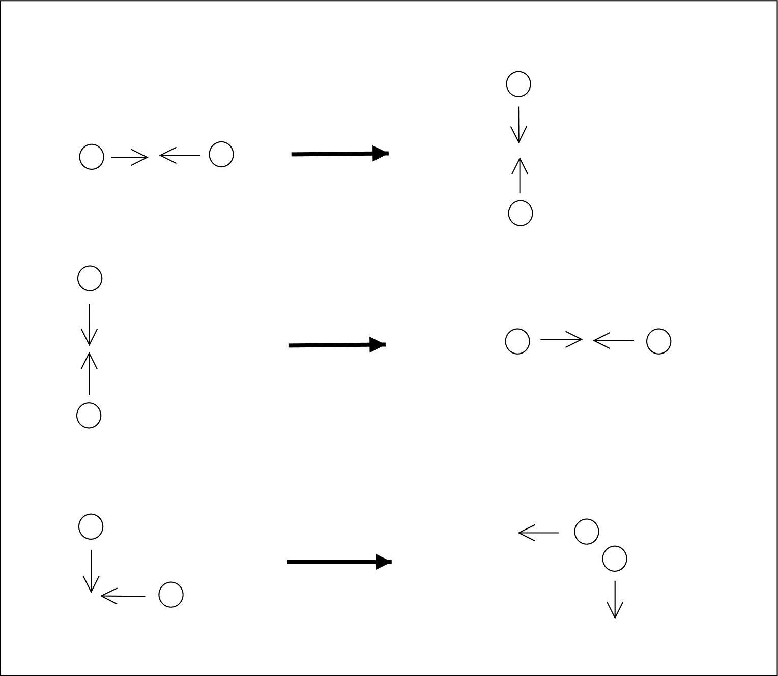
Figure 4: Collisions in the HPP lattice gas rule. Horizontal collisions produce vertically-moving particles (top) and vice versa (middle). Particles moving at right angles pass by each other unchanged (bottom, omitting the reflections and rotations of this figure).

5 Agent-Based Models

If there is any one technique associated with complex systems science, it is agent-based modeling. An agent-based model is a computational model which represents individual agents and their collective behavior. What, exactly, do we mean by “agent”? Stuart Kauffman has offered the following apt definition: “An agent is a thing which does things to things”. That is, an agent is a persistent thing which has some state we find worth representing, and which interacts with other agents, mutually modifying each others’ states. The components of an agent-based model are a collection of agents and their states, the rules governing the interactions of the agents, and the environment within which they live. (The environment need not be represented in the model if its effects are constant.) The state of an agent can be arbitrarily simple, say just position, or the color of a cell in a CA. (At this end, agent-based models blend with traditional stochastic models.) States can also be extremely complicated, including, possibly, sophisticated internal models of the agent’s world.

Here is an example to make this concrete. In epidemiology, there is a classic kind of model of the spread of a disease through a population called an “SIR” model [Bartlett-stochastic, §4.4]. It has three classes of people — the susceptible, who have yet to be exposed to the disease; the infected, who have it and can pass it on; and the resistant or recovered, who have survived the disease and cannot be re-infected. A traditional approach to an SIR model would have three variables, namely the number of people in each of the three categories, $S(t),I(t),R(t)$, and would have some deterministic or stochastic dynamics in terms of those variables. For instance, in a deterministic SIR model, one might have

$$S(t+1)-S(t) = -a\left(\frac{I(t)}{S(t)+I(t)+R(t)}\right)S(t)$$ (36)

$$I(t+1)-I(t) = \left[a\frac{S(t)}{S(t)+I(t)+R(t)}-b-c\right]I(t)$$ (37)

$$R(t+1)-R(t) = bI(t)$$ (38)

which we could interpret by saying that (i) the probability of a susceptible person being infected is proportional to the fraction of the population which is already infected, (ii) infected people get better at a rate $b$ and (iii) infected people die at a rate $c$. (This is not a particularly realistic SIR model.) In a stochastic model, we would treat the right hand sides of (36)–(38) as the mean changes in the three variables, with (say) Poisson-distributed fluctuations, taking care that, e.g., the fluctuation in the $a\frac{I}{R+S+I}$ term in (36) is the same as that in (37). The thing to note is that, whether deterministic or stochastic, the whole model is cast in terms of the aggregate quantities $S$, $I$ and $R$, and those aggregate variables are what we would represent computationally.

In an agent-based model of the same dynamics, we would represent each individual in the population as a distinct agent, which could be in one of three states, S, I and R. A simple interaction rule would be that at each time-step, each agent selects another from the population entirely at random. If a susceptible agent (i.e., one in state S) picks an infectious agent (i.e., one in state I), it becomes infected with probability $a$. Infectious agents die with probability $b$ and recover with probability $c$; recovered agents never change their state.

So far, we have merely reproduced the stochastic version of (36)–(38), while using many more variables. The power of agent-based modeling only reveals itself when we implement more interesting interaction rules. For instance, it would be easy to assign each agent a position, and make two agents more likely to interact if they are close. We could add visible symptoms which are imperfectly associated with the disease, and a tendency not to interact with symptomatic individuals. We could make the degree of aversion to symptomatic agents part of the agents’ state. All of this is easy to implement in the model, even in combination, but not easy to do in a more traditional, aggregated model. Sometimes it would be all but impossible; an excellent case in point is the highly sophisticated model of HIV epidemiology produced by Jacquez, Koopman, Simon and collaborators [Jacquez-et-al-on-HIV, Koopman-et-al-on-HIV], incorporating multiple routes of transmission, highly non-random mixing of types, and time-varying infectiousness.

Agent-based models steer you towards representing individuals, their behaviors and their interactions, rather than aggregates and their dynamics. Whether this is a good thing depends, of course, on what you know, and what you hope to learn. If you know a lot about individuals, agent-based models can help you leverage that knowledge into information about collective dynamics. This is particularly helpful if the population is heterogeneous, since you can represent the different types of individuals in the population by different states for agents. This requires a bit of effort on your part, but often not nearly so much as it would to represent the heterogeneity in an aggregated model. Conversely, if you think you have the collective dynamics down, an ABM will let you check whether a candidate for an individual-level mechanism really will produce them. (But see §6, below.)

Ideally, there are no “mass nouns” in an ABM, nothing represented by a smeared-out “how much”: everything should be represented by some definite number of distinctly-located agents. At most, some aggregate variables may be stuffed into the environment part of the model, but only simple and homogeneous ones. Of course, the level of disaggregation at which it is useful to call something an agent is a matter for particular applications, and need not be the same for every agent in a model. (E.g., one might want to model an entire organ as a single agent, while another, more interesting organ is broken up into multiple interacting agents, along anatomical or functional lines.) Sometimes it’s just not practical to represent everything which we know is an individual thing by its own agent: imagine trying to do chemical thermodynamics by tracking the interactions of a mole of molecules. Such cases demand either giving up on agent-based modeling (fortunately, the law of mass action works pretty well in chemistry), or using fictitious agents that represent substantial, but not too large, collections of individuals.

Models describing the collective dynamics of aggregate variables are sometimes called “equation-based models”, in contrast to agent-based models. This is sloppy, however: it is always possible, though generally tedious and unilluminating, to write down a set of equations which describe the dynamics of an agent-based model. Rather than drawing a false contrast between agents and equations, it would be better to compare ABMs to “aggregate models”, “collective models” or perhaps “factor models”.

5.1 Computational Implementation: Agents are Objects

The nicest way to computationally implement the commitment of distinctly representing each agent, is to make agents objects, which are, to over-simplify slightly, data structures which have internal states, and interact with each other by passing messages. While objects are not necessary for agent-based models, they do make programming them much easier, especially if the agents have much more state than, say, just a position and a type. If you try to implement models with sophisticated agents without using objects, the odds are good that you will find yourself re-inventing well-known features of object-oriented programming. (Historically, object-oriented programming began with languages for simulation modeling [Budd-understanding-oop].) You might as well save your time, and do those things right, by using objects in the first place.

Generally speaking, computational implementations of ABMs contain many non-agent objects, engaged in various housekeeping tasks, or implementing the functions agents are supposed to perform. For instance, an agent, say a rat, might be supposed to memorize a sequence, say of turns in a maze. One way of implementing this would be to use a linked list, which is an object itself. Such objects do not represent actual features of the model, and it should be possible to vary them without interfering with the model’s behavior. Which objects are picked out as agents is to some degree a matter of convenience and taste. It is common, for instance, to have mobile agents interacting on a static environment. If the environment is an object, modelers may or may not speak of it as an “environment agent,” and little seems to hinge on whether or not they do.

There are several programming environments designed to facilitate agent-based modeling. Perhaps the best known of these is Swarm (www.swarm.org), which works very flexibly with several languages, is extensively documented, and has a large user community, though it presently (2004) lacks an institutional home. RePast, while conceptually similar, is open-source (repast.sourceforge.net) and is associated with the University of Chicago. StarLogo, and it successor, NetLogo (ccl.sesp.northwestern.edu/netlogo), are extensions of the popular Logo language to handle multiple interacting “turtles”, i.e., agents. Like Logo, children can learn to use them [Resnick-turtles], but they are fairly easy for adults, too, and certainly give a feel for working with ABMs.

5.2 Three Things Which Are Not Agent-Based Models

Not everything which involves the word “agent” is connected to agent-based modeling.

Representative agent models are not ABMs. In these models, the response of a population to environment conditions is found by picking out a single typical or representative agent, determining their behavior, and assuming that everyone else does likewise. This is sometimes reasonable, but it’s clearly diametrically opposed to what an ABM is supposed to be.

Software agents are not ABMs. Software agents are a very useful and rapidly developing technology [Brown-Duguid-SLoI, chapter 2]; an agent, here, is roughly a piece of code which interacts with other software and with pieces of the real world autonomously. Agents index the Web for search engines, engage in automated trading, and help manage parts of the North American electrical power grid, among other things. Some agent software systems are inspired by ABMs [Bonabeau-Dorigo-Theraulaz-swarm-intelligence]. When one wants to model their behavior, an ABM is a natural tool (but not the only one by any means: see [Lerman-design-and-analysis]). But a set of software agents running the Michigan power grid is not a model of anything, it’s doing something.

Finally, multi-agent systems [Ossowski-artificial-agent-societies] and rational agents [Wooldridge-reasoning] in artificial intelligence are not ABMs. The interest of this work is in understanding, and especially designing, systems capable of sophisticated, autonomous cognitive behavior; many people in this field would restrict the word “agent” to apply only to things capable, in some sense, of having “beliefs, desires and intentions”. While these are certainly complex systems, they are not usually intended to be models of anything else. One can, of course, press them into service as models [Jonker-et-al-intentions-in-biochemistry], but generally this will be no more than a heuristic device.

5.3 The Simplicity of Complex Systems Models

One striking feature of agent-based models, and indeed of complex systems models in general, is how simple they are. Often, agents have only a few possible states, and only a handful of kinds of interaction. This practice has three motivations. (i) A model as detailed as the system being studied would be as hard to understand as that system. (ii) Many people working in complex systems science want to show that a certain set of mechanisms are sufficient to generate some phenomenon, like cooperation among unrelated organisms, or the formation of striped patterns. Hence using simple models, which contain only those mechanisms, makes the case. (iii) Statistical physicists, in particular, have a long tradition of using highly simplified models as caricatures of real systems.

All three motives are appropriate, in their place. (i) is completely unexceptionable; abstracting away from irrelevant detail is always worthwhile, so long as it really is irrelevant. (ii) is also fair enough, though one should be careful that the mechanisms in one’s model can still generate the phenomenon when they interact with other effects as well. (iii) works very nicely in statistical physics itself, where there are powerful mathematical results relating to the renormalization group [Chaikin-Lubensky] and bifurcation theory [Cross-Hohenberg] which allow one to extract certain kinds of quantitative results from simplified models which share certain qualitative characteristics with real systems. (We have seen a related principle when discussing cellular automata models above.) There is, however, little reason to think that these universality results apply to most complex systems, let alone ones with adaptive agents!

6 Evaluating Models of Complex Systems

We do not build models for their own sake; we want to see what they do, and we want to compare what they do both to reality and to other models. This kind of evaluation of models is a problem for all areas of science, and as such little useful general advice can be given. However, there are some issues which are peculiar to models of complex systems, or especially acute for them, and I will try to provide some guidance here, moving from figuring out just what your model does, to comparing your model to data, to comparing it to other models.

6.1 Simulation

The most basic way to see what your model does is to run it; to do a simulation. Even though a model is entirely a human construct, every aspect of its behavior following logically from its premises and initial conditions, the frailty of human nature is such that we generally cannot perceive those consequences, not with any accuracy. If the model involves a large number of components which interact strongly with each other — if, that is to say, it’s a good model of a complex system — our powers of deduction are generally overwhelmed by the mass of relevant, interconnected detail. Computer simulation then comes to our aid, because computers have no trouble remembering large quantities of detail, nor in following instructions.

6.1.1 Direct Simulation

Direct simulation — simply starting the model and letting it go — has two main uses. One is to get a sense of the typical behavior, or of the range of behavior. The other, more quantitative, use is to determine the distribution of important quantities, including time series. If one randomizes initial conditions, and collects data over multiple runs, one can estimate the distribution of desired quantities with great accuracy. This is exploited in the time series method of surrogate data (above), but the idea applies quite generally.

Individual simulation runs for models of complex systems can be reasonably expensive in terms of time and computing power; large numbers of runs, which are really needed to have confidence in the results, are correspondingly more costly. Few things are more dispiriting than to expend such quantities of time and care, only to end up with ambiguous results. It is almost always worthwhile, therefore, to carefully think through what you want to measure, and why, before running anything. In particular, if you are trying to judge the merits of competing models, effort put into figuring out how and where they are most different will generally be well-rewarded. The theory of experimental design offers extensive guidance on how to devise informative series of experiments, both for model comparison and for other purposes, and by and large the principles apply to simulations as well as to real experiments.

6.1.2 Monte Carlo Methods

Monte Carlo is the name of a broad, slightly indistinct family for using random processes to estimate deterministic quantities, especially the properties of probability distributions. A classic example will serve to illustrate the basic idea, on which there are many, many refinements.

Consider the problem of determining the area $A$ under an curve given by a known but irregular function $f(x)$. In principle, you could integrate $f$ to find this area, but suppose that numerical integration is infeasible for some reason. (We will come back to this point presently.) A Monte Carlo solution to this problem is as follows: pick points at random, uniformly over the square. The probability $p$ that a point falls in the shaded region is equal to the fraction of the square occupied by the shading: $p=A/s^{2}$. If we pick $n$ points independently, and $x$ of them fall in the shaded region, then $x/n\rightarrow p$ (by the law of large numbers), and $s^{2}x/n\rightarrow A$. $s^{2}x/n$ provides us with a stochastic estimate of the integral. Moreover, this is a probably approximately correct (§2.1.3) estimate, and we can expect, from basic probability theory, that the standard deviation of the estimate around its true value will be proportional to $n^{-1/2}$, which is not bad. However, when faced with such a claim, one should always ask what the proportionality constant is, and whether it is the best achievable. Here it is not: the equally simple, if less visual, scheme of just picking values of $x$ uniformly and averaging the resulting values of $f(x)$ always has a smaller standard deviation [Hammersley-Handscomb, chapter 5].

This example, while time-honored and visually clear, does not show Monte Carlo to its best advantage; there are few one-dimensional integrals which cannot be done better by ordinary, non-stochastic numerical methods. But numerical integration becomes computationally intractable when the domain of integration has a large number of dimensions, where “large” begins somewhere between four and ten. Monte Carlo is much more indifferent to the dimensionality of the space: we could replicate our example with a 999-dimensional hyper-surface in a 1000-dimensional space, and we’d still get estimates that converged like $n^{-1/2}$, so achieving an accuracy of $\pm\epsilon$ will require evaluating the function $f$ only $O(\epsilon^{-2})$ times.

Our example was artificially simple in another way, in that we used a uniform distribution over the entire space. Often, what we want is to compute the expectation of some function $f(x)$ with a non-uniform probability $p(x)$. This is just an integral, $\int{f(x)p(x)dx}$, so we could sample points uniformly and compute $f(x)p(x)$ for each one. But if some points have very low probability, so they only make a small contribution to the integral, spending time evaluating the function there is a bit of a waste. A better strategy would be to pick points according to the actual probability distribution. This can sometimes be done directly, especially if $p(x)$ is of a particularly nice form. A very general and clever indirect scheme is as follows [Metropolis-et-al-Monte-Carlo]. We want a whole sequence of points, $x_{1},x_{2},\ldots x_{n}$. We pick the first one however we like, and after that we pick successive points according to some Markov chain: that is, the distribution of $x_{i+1}$ depends only on $x_{i}$, according to some fixed function $q(x_{i},x_{i+1})$. Under some mild conditions, the distribution of $x_{t}$ approaches a stationary distribution $q^{*}(x)$ at large times $t$. If we could ensure that $q^{*}(x)=p(x)$, we know that the Markov chain was converging to our distribution, and then, by the ergodic theorem, averaging $f(x)$ along a trajectory would give the expected value of $f(x)$. One way to ensure this is to use the “detailed balance” condition of the invariant distribution, that the total probability of going from $x$ to $y$ must equal the total probability of going the other way:

$$p(x)q(x,y) = p(y)q(y,x)$$ (39)

$$\frac{q(x,y)}{q(y,x)} = \frac{p(y)}{p(x)}\equiv h(x,y)$$ (40)

So now we just need to make sure that (40) is satisfied. One way to do this is to set $q(x,y)=\min{\left(1,h(x,y)\right)}$; this was the original proposal of Metropolis et al. Another is $q(x,y)=\frac{h(x,y)}{1+h(x,y)}$. This method is what physicists usually mean by “Monte Carlo”, but statisticians call it Markov chain Monte Carlo, or “MCMC”. While we can now estimate the properties of basically arbitrary distributions, we no longer have independent samples, so evaluating the accuracy of our estimates is no longer a matter of trivial probability. An immense range of refinements have been developed over the last fifty years, addressing these and other points; see the further reading section for details.

Keep in mind that Monte Carlo is a stochastic simulation method only in a special sense — it simulates the probability distribution $p(x)$, not the mechanism which generated that distribution. The dynamics of Markov chain Monte Carlo, in particular, often bear no resemblance whatsoever to those of the real system. Since the point of Monte Carlo is to tell us about the properties of $p(x)$ (what is the expectation value of this function? what is the probability of configurations with this property? etc.), the actual trajectory of the Markov chain is of no interest. This point sometimes confuses those more used to direct simulation methods.

6.2 Analytical Techniques

Naturally enough, analytical techniques are not among the tools which first come to mind for dealing with complex systems; in fact, they often do not come to mind at all. This is unfortunate, because a lot of intelligence has been devoted to devising approximate analytical techniques for classes of models which include many of those commonly used for complex systems. A general advantage of analytical techniques is that they are often fairly insensitive to many details of the model. Since any model we construct of a complex system is almost certainly much simpler than the system itself, a great many of its details are just wrong. If we can extract non-trivial results which are insensitive to those details, we have less reason to worry about this.

One particularly useful, yet neglected, body of approximate analytical techniques relies on the fact that many complex systems models are Markovian. In an agent-based model, for instance, the next state of an agent generally depends only on its present state, and the present states of the agents it interacts with. If there is a fixed interaction graph, the agents form a Markov random field on that graph. There are now very powerful and computationally efficient methods for evaluating many properties of Markov chains [Honerkamp-stochastic, Bremaud-markov-chains], Markov random fields [Beckerman-adaptive], and (closely related) graphical models [Jordan-learning-in-graphical-models] without simulation. The recent books of Peyton Young [Young-strategy-structure] and Sutton [Sutton-technology-and-market-structure] provide nice instances of using analytical results about Markov processes to solve models of complex social systems, without impractical numerical experiments.

6.3 Comparisons with Data

6.3.1 General issues

We can only compare particular aspects of a model of a system to particular kinds of data about that system. The most any experimental test can tell us, therefore, is how similar the model is to the system in that respect. One may think of an experimental comparison as a test for a particular kind of error, one of the infinite number of mistakes which we could make in building a model. A good test is one which is very likely to alert us to an error, if we have made it, but not otherwise [Mayo-error].

These ought to be things every school-child knows about testing hypotheses. It is very easy, however, to blithely ignore these truisms when confronted with, on the one hand, a system with many strongly interdependent parts, and, on the other hand, a model which tries to mirror that complexity. We must decide which features of the model ought to be similar to the system, and how similar. It is important not only that our model be able to adequately reproduce those phenomena, but that it not entail badly distorted or non-existent phenomena in other respects.

6.3.2 Two Stories and Some Morals

Let me give two examples from very early in the study of complex systems, which nicely illustrate some fundamental points.

The first has to do with pattern formation in chemical oscillators [Epstein-Pojman]. Certain mixtures of chemicals in aqueous solution, mostly famously the Belusov-Zhabotinsky reagent, can not only undergo cyclic chemical reactions, but will form rotating spiral waves, starting from an initial featureless state. This is a visually compelling example of self-organization, and much effort has been devoted to understanding it. One of the more popular early models was the “Brusselator” advanced by Prigogine and his colleagues at the Free University of Brussels; many similarly-named variants developed. Brusselator-type models correctly predicted that these media would support spiral waves. They all, further, predicted that the spirals would form only when the homogeneous configuration was unstable, and that then they would form spontaneously. It proved very easy, however, to prepare the Belusov-Zhabotisnky reagent in such a way that it was “perfectly stable in its uniform quiescence”, yet still able to produce spiral waves if excited (e.g., by being touched with a hot wire) [Winfree-time-breaks-down]. The Brusselator and its variants were simply unable to accommodate these phenomena, and had to be discarded in favor of other models. The fact that these were qualitative results, rather than quantitative ones, if anything made it more imperative to get rid of the Brusselator.

The second story concerns the work of Varela and Maturana on “autopoesis”. In a famous paper [Varela-Maturana-Uribe], they claimed to exhibit a computational model of a simple artificial chemistry where membranes not only formed spontaneously, but a kind of metabolism self-organized to sustain the membranes. This work influenced not just complex systems science but theoretical biology, psychology, and even sociology [Luhmann-social-systems]. When, in the 1990s, McMullin made the first serious effort to reproduce the results, based on the description of the model in the paper, that description proved not to match the published simulation results. The discrepancy was only resolved by the fortuitous rediscovery of a mass of papers, including Fortran code, that Varela had left behind in Chile when forced into exile by the fascist regime. These revealed a crucial change in one particular reaction made all the difference between successful autopoesis and its absence. (For the full story, see [McMullin-independent, McMullin-Varela].) Many similar stories could be told of other models in complex systems [Revisiting-edge-of-chaos]; this one is distinguished by McMullin’s unusual tenacity in trying to replicate the results, Varela’s admirable willingness to assist him, and the happy ending.

The story of autopoesis is especially rich in morals. (1) Replication is essential. (2) It is a good idea to share not just data but programs. (3) Always test the robustness of your model to changes in its parameters. (This is fairly common.) (4) Always test your model for robustness to small changes in qualitative assumptions. If your model calls for a given effect, there are usually several mechanisms which could accomplish it. If it does not matter which mechanism you actually use, the result is that much more robust. Conversely, if it does matter, the over-all adequacy of the model can be tested by checking whether that mechanism is actually present in the system. Altogether too few people perform such tests.

6.3.3 Comparing Macro-data and Micro-models

Data are often available only about large aggregates, while models, especially agent-based models, are about individual behavior. One way of comparing such models to data is to compute the necessary aggregates, from direct simulation, Monte Carlo, etc. The problem is that many different models can give the same aggregated behavior, so this does not provide a powerful test between different models. Ideally, we’d work back from aggregate data to individual behaviors, which is known, somewhat confusingly, as ecological inference. In general, the ecological inference problem itself does not have a unique solution. But the aggregate data, if used intelligently, can often put fairly tight constraints on the individual behaviors, and micro-scale can be directly checked against those constraints. Much of the work here has been done by social scientists, especially American political scientists concerned with issues arising from the Voting Rights Act [Schuessler-ecological-inference], but the methods they have developed are very general, and could profitably be applied to agent-based models in the biological sciences, though, to my knowledge, they have yet to be.

6.4 Comparison to Other Models

Are there other ways of generating the data? There generally are, at least if “the data” are some very gross, highly-summarized pattern. This makes it important to look for differential signatures, places where discrepancies between different generative mechanisms give one some leverage. Given two mechanisms which can both account for our phenomenon, we should look for some other quantity whose behavior will be different under the two hypotheses. Ideally, in fact, we would look for the statistic on which the two kinds of model are most divergent. The literature on experimental design is relevant here again, since it considers such problems under the heading of model discrimination, seeking to maximize the power of experiments (or simulations) to distinguish between different classes of models [Atkinson-Donev, Borowiak-model-discrimination].

Perhaps no aspect of methodology is more neglected in complex systems science than this one. While it is always perfectly legitimate to announce a new mechanism as a way of generating a phenomenon, it is far too common for it to be called the way to do it, and vanishingly rare to find an examination of how it differs from previously-proposed mechanisms. Newman and Palmer’s work on extinction models [MEJN-Palmer-extinctions] stands out in this regard for its painstaking examination of the ways of discriminating between the various proposals in the literature.

7 Information Theory

Information theory began as a branch of communications engineering, quantifying the length of codes needed to represent randomly-varying signals, and the rate at which data can be transmitted over noisy channels. The concepts needed to solve these problems turn out to be quite fundamental measures of the uncertainty, variability, and the interdependence of different variables. Information theory thus is an important tool for studying complex systems, and in addition is indispensable for understanding complexity measures (§8).

7.1 Basic Definitions

Our notation and terminology follows that of Cover and Thomas’s standard textbook [Cover-and-Thomas].

Given a random variable $X$ taking values in a discrete set $\mathcal{A}$, the entropy or information content $H[X]$ of $X$ is

$$H[X] \equiv -\sum_{a\in\mathcal{A}}{\mathrm{Pr}(X=a)\log_{2}{\mathrm{Pr}(X=a)}}~{}.$$ (41)

$H[X]$ is the expectation value of $-\log_{2}{\mathrm{Pr}(X)}$. It represents the uncertainty in $X$, interpreted as the mean number of binary distinctions (bits) needed to identify the value of $X$. Alternately, it is the minimum number of bits needed to encode or describe $X$. Note that $H[X]=0$ if and only if $X$ is (almost surely) constant.

The joint entropy $H[X,Y]$ of two variables $X$ and $Y$ is the entropy of their joint distribution:

$$H[X,Y] \equiv -\sum_{a\in\mathcal{A},b\in\mathcal{B}}{\mathrm{Pr}(X=a,Y=b)\log_{2}{\mathrm{Pr}(X=a,Y=b)}}~{}.$$ (42)

The conditional entropy of $X$ given $Y$ is

$$H[X|Y] \equiv H[X,Y]-H[Y]~{}.$$ (43)

$H[X|Y]$ is the average uncertainty remaining in $X$, given a knowledge of $Y$.

The mutual information $I[X;Y]$ between $X$ and $Y$ is

$$I[X;Y] \equiv H[X]-H[X|Y]~{}.$$ (44)

It gives the reduction in $X$’s uncertainty due to knowledge of $Y$ and is symmetric in $X$ and $Y$. We can also define higher-order mutual informations, such as the third-order information $I[X;Y;Z]$,

$$I[X;Y;Z] \equiv H[X]+H[Y]+H[Z]-H[X,Y,Z]$$ (45)

and so on for higher orders. These functions reflect the joint dependence among the variables.

Mutual information is a special case of the relative entropy, also called the Kullback-Leibler divergence (or distance). Given two distributions (not variables), $\mathrm{P}$ and $\mathrm{Q}$, the entropy of $\mathrm{Q}$ relative to $\mathrm{P}$ is

$$D(\mathrm{P}\|\mathrm{Q}) \equiv \sum_{x}{\mathrm{P}(x)\log{\frac{\mathrm{P}(x)}{\mathrm{Q}(x)}}}$$ (46)

$D$ measures how far apart the two distributions are, since $D(\mathrm{P}||\mathrm{Q})\geq 0$, and $D(\mathrm{P}\|\mathrm{Q})=0$ implies the two distributions are equal almost everywhere. The divergence can be interpreted either in terms of codes (see below), or in terms of statistical tests [Kullback-info-theory-and-stats]. Roughly speaking, given $n$ samples drawn from the distribution $\mathrm{P}$, the probability of our accepting the false hypothesis that the distribution is $\mathrm{Q}$ can go down no faster than $2^{-nD(\mathrm{P}\|\mathrm{Q})}$. The mutual information $I[X;Y]$ is the divergence between the joint distribution $\mathrm{Pr}(X,Y)$, and the product of the marginal distributions, $\mathrm{Pr}(X)\mathrm{Pr}(Y)$, and so measures the departure from independence.

Some extra information-theoretic quantities make sense for time series and stochastic processes. Supposing we have a process $\bar{X}=$
$\ldots,X_{-2},X_{-1},X_{0},X_{1},X_{2},\ldots$, we can define its mutual information function by analogy with the autocovariance function (see §3.2),

$$I_{\bar{X}}(s,t) = I[X_{s};X_{t}]$$ (47)

$$I_{\bar{X}}(\tau) = I[X_{t};X_{t+\tau}]$$ (48)

where the second form is valid only for strictly stationary processes. The mutual information function measures the degree to which different parts of the series are dependent on each other.

The entropy rate $h$ of a stochastic process

$$h \equiv \lim_{L\rightarrow\infty}{H[X_{0}|X_{-L}^{-1}]}$$ (49)

$$= H[X_{0}|X_{-\infty}^{-1}]~{}.$$ (50)

(The limit always exists for stationary processes.) $h$ measures the process’s unpredictability, in the sense that it is the uncertainty which remains in the next measurement even given complete knowledge of its past. In nonlinear dynamics, $h$ is called the Kolmogorov-Sinai (KS) entropy.

For continuous variables, one can define the entropy via an integral,

$$H[X] \equiv -\int{p(x)\log{p(x)}dx}~{},$$ (51)

with the subtlety that the continuous entropy not only can be negative, but depends on the coordinate system used for $x$. The relative entropy also has the obvious definition,

$$D(\mathrm{P}\|\mathrm{Q}) \equiv \int{p(x)\log{\frac{p(x)}{q(x)}}dx}$$ (52)

but is coordinate-independent and non-negative. So, hence, is the mutual information.

Optimal Coding

One of the basic results of information theory concerns codes, or schemes for representing random variables by bit strings. That is, we want a scheme which associates each value of a random variable $X$ with a bit string. Clearly, if we want to keep the average length of our code-words small, we should give shorter codes to the more common values of $X$. It turns out that the average code-length is minimized if we use $-\log{\mathrm{Pr}(x)}$ bits to encode $x$, and it is always possible to come within one bit of this. Then, on average, we will use $\mathbf{E}\left[-\log{\mathrm{Pr}(x)}\right]=H[X]$ bits.

This presumes we know the true probabilities. If we think the true distribution is $\mathrm{Q}$ when it is really $\mathrm{P}$, we will, on average, use $\mathbf{E}\left[-\log{\mathrm{Q}(x)}\right]\geq H[X]$. This quantity is called the cross-entropy or inaccuracy, and is equal to $H[X]+D(\mathrm{P}\|\mathrm{Q})$. Thus, finding the correct probability distribution is equivalent to minimizing the cross-entropy, or the relative entropy [Kulhavy-recursive].

The Khinchin Axioms and Rényi Information

In 1953, A. I. Khinchin published a list of four reasonable-looking axioms for a measure of the information $H[X]$ associated with a random variable $X$ [Khinchin-info]. He then proved that the Shannon information was the unique functional satisfying the axioms, up to an over-all multiplicative constant. (The choice of this constant is equivalent to the choice of the base for logarithms.) The axioms were as follows.

• The information is a functional of the probability distribution of $X$, and not on any of its other properties. In particular, if $f$ is any invertible function, $H[X]=H[f(X)]$.

• The information is maximal for the uniform distribution, where all events are equally probable.

• The information is unchanged by enlarging the probability space with events of zero probability.

• If the probability space is divided into two sub-spaces, so that $X$ is split into two variables $Y$ and $Z$, the total information is equal to the information content of the marginal distribution of one sub-space, plus the mean information of the conditional distribution of the other sub-space: $H[X]=H[Y]+\mathbf{E}\left[H(Z|Y)\right]$.

A similar axiomatic treatment can be given for the mutual information and the relative entropy.

While the first three of Khinchin’s axioms are all highly plausible, the fourth is somewhat awkward. It is intuitively more plausible to merely require that, if $Y$ and $Z$ are independent, then $H[Y,Z]=H[Y]+H[Z]$. If the fourth axiom is weakened in this way, however, there is no longer only a single functional satisfying the axioms. Instead, any of the infinite family of entropies introduced by Rényi satisfies the axioms. The Rényi entropy of order $\alpha$, with $\alpha$ any non-negative real number, is

$$H_{\alpha}[X] \equiv \frac{1}{1-\alpha}{\log{\sum_{i:p_{i}>0}{p_{i}^{\alpha}}}}$$ (53)

in the discrete case, and the corresponding integral in the continuous case. The parameter $\alpha$ can be thought of as gauging how strongly the entropy is biased towards low-probability events. As $\alpha\rightarrow 0$, low-probability events count more, until at $\alpha=0$, all possible events receive equal weight. (This is sometimes called the topological entropy.) As $\alpha\rightarrow\infty$, only the highest-probability event contributes to the sum. One can show that, as $\alpha\rightarrow 1$, $H_{\alpha}[X]\rightarrow H[X]$, i.e., one recovers the ordinary Shannon entropy in the limit. There are entropy rates corresponding to all the Rényi entropies, defined just like the ordinary entropy rate. For dynamical systems, these are related to the fractal dimensions of the attractor [Ruelle-Lincei, Beck-Schlogl].

The Rényi divergences bear the same relation to the Rényi entropies as the Kullback-Leibler divergence does to the Shannon entropy. The defining formula is

$$D_{\alpha}(\mathrm{P}||\mathrm{Q}) \equiv \frac{1}{\alpha-1}\log{\sum{q_{i}{\left(\frac{p_{i}}{q_{i}}\right)}^{\alpha}}}$$ (54)

and similarly for the continuous case. Once again, $\lim_{\alpha\rightarrow 1}{D_{\alpha}(\mathrm{P}||\mathrm{Q})}=D(\mathrm{P}||\mathrm{Q})$. For all $\alpha>0$, $D_{\alpha}(\mathrm{P}||\mathrm{Q})\geq 0$, and is equal to zero if and only if $\mathrm{P}$ and $\mathrm{Q}$ are the same. (If $\alpha=0$, then a vanishing Rényi divergence only means that the supports of the two distributions are the same.) The Rényi entropy $H_{\alpha}[X]$ is non-increasing as $\alpha$ grows, whereas the Rényi divergence $D_{\alpha}(\mathrm{P}||\mathrm{Q})$ is non-decreasing.

Estimation of Information-Theoretic Quantities

In applications, we will often want to estimate information-theoretic quantities, such as the Shannon entropy or the mutual information, from empirical or simulation data. Restricting our attention, for the moment, to the case of discrete-valued variables, the empirical distribution will generally converge on the true distribution, and so the entropy (say) of the empirical distribution (“sample entropy”) will also converge on the true entropy. However, it is not the case that the sample entropy is an unbiased estimate of the true entropy. The Shannon (and Rényi) entropies are measures of variation, like the variance, and sampling tends to reduce variation. Just as the sample variance is a negatively biased estimate of the true variance, sample entropy is a negatively-biased estimate of the true entropy, and so sample mutual information is a positively-biased estimate of true information. Understanding and controlling the bias, as well as the sampling fluctuations, can be very important.

Victor [Victor-information-bias] has given an elegant method for calculating the bias of the sample entropy; remarkably, the leading-order term depends only on the alphabet size $k$ and the number of samples $N$, and is $(k-1)/2N$. Higher-order terms, however, depend on the true distribution. Recently, Kraskov et al. [Kraskov-et-al-estimating-MI] have published an adaptive algorithm for estimating mutual information, which has very good properties in terms of both bias and variance. Finally, the estimation of entropy rates is a somewhat tricky matter. The best practices are to either use an algorithm of the type given by [Kontoyiannis-et-al-estimating-entropy-rate], or to fit a properly dynamical model. (For discrete data, variable-length Markov chains, discussed in §3.6.2 above, generally work very well, and the entropy rate can be calculated from them very simply.) Another popular approach is to run one’s time series through a standard compression algorithm, such as gzip, dividing the size in bits of the output by the number of symbols in the input [Benedetto-et-al-language-trees]. This is an absolutely horrible idea; even under the circumstances under which it gives a consistent estimate of the entropy rate, it converges much more slowly, and runs more slowly, than employing either of the two techniques just mentioned [Khmelev-Teahan-on-Benedetto-et-al, Goodman-on-Benedetto-et-al].

7.2 Applications of Information Theory

Beyond its original home in communications engineering, information theory has found a multitude of applications in statistics [Kullback-info-theory-and-stats, Kulhavy-recursive] and learning theory [Jordan-learning-in-graphical-models, MacKay-learning-algorithms]. Scientifically, it is very natural to consider some biological systems as communications channels, and so analyze their information content; this has been particularly successful for biopolymer sequences [Bio-sequence-analysis] and especially for neural systems, where the analysis of neural codes depends vitally on information theory [Spikes-book, Abbott-Sejnowski-neural-codes]. However, there is nothing prohibiting the application of information theory to systems which are not designed to function as communications devices; the concepts involved require only well-defined probability distributions. For instance, in nonlinear dynamics [Billingsley-ergodic-theory-and-info, Katok-Hasselblatt] information-theoretic notions are very important in characterizing different kinds of dynamical system (see also §3.6). Even more closely tied to complex systems science is the literature on “physics and information” or “physics and computation”, which investigates the relationships between the mechanical principles of physics and information theory, e.g., Landauer’s principle, that erasing (but not storing) a bit of information at temperature $T$ produces $k_{B}T\ln{2}$ joules of heat, where $k_{B}$ is Boltzmann’s constant.

8 Complexity Measures

We have already given some thought to complexity, both in our initial rough definition of “complex system” and in our consideration of machine learning and Occam’s Razor. In the latter, we saw that the relevant sense of “complexity” has to do with families of models: a model class is complex if it requires large amounts of data to reliably find the best model in the class. On the other hand, we initially said that a complex system is one with many highly variable, strongly interdependent parts. Here, we will consider various proposals for putting some mathematical spine into that notion of a system’s complexity, as well as the relationship to the notion of complexity of learning.

Most measures of complexity for systems formalize the intuition that something is complex if it is difficult to describe adequately. The first mathematical theory based on this idea was proposed by Kolmogorov; while it is not good for analyzing empirical complex systems, it was very important historically, and makes a good point of entry into the field.

8.1 Algorithmic Complexity

Consider a collection of measured data-values, stored in digitized form on a computer. We would like to say that they are complex if they are hard to describe, and measure their complexity by the difficulty of describing them. The central idea of Kolmogorov complexity (proposed independently by Solomonoff [Solomonoff] and Chaitin) is that one can describe the data set by writing a program which will reproduce the data. The difficulty of description is then measured by the length of the program. Anyone with much experience of other people’s code will appreciate that it is always possible to write a longer, slower program to do a given job, so what we are really interested in is the shortest program that can exactly replicate the data.

To introduce some symbols, let $x$ be the data, and $|x|$ their size in bits. The Kolmogorov or algorithmic complexity of $x$, $K(x)$, is the length of the shortest program that will output $x$ and then stop. Clearly, there is always some program which will output $x$ and then stop, for instance, “print($x$); end”. Thus $K(x)\leq|x|+c$, where $c$ is the length of the print and end instructions. This is what one might call a literal description of the data. If one cannot do better than this — if $K(x)\approx|x|$ — then $x$ is highly complex. Some data, however, is highly compressible. For instance, if $x$ consists of the second quadrillion digits of $\pi$, a very short program suffices to generate it.

As you may already suspect, the number of simple data sets is quite limited. Suppose we have a data set of size $n$ bits, and we want to compress it by $k$ bits, i.e., find a program for it which is $n-k$ bits long. There are at most $2^{n-k}$ programs of that length, so of all the $2^{n}$ data sets of size $n$, the fraction which can be compressed by $k$ bits is at most $2^{-k}$. The precise degree of compression does not matter — when we look at large data sets, almost all of them are highly complex. If we pick a large data set at random, then the odds are very good that it will be complex. We can state this more exactly if we think about our data as consisting of the first $n$ measurements from some sequence, and let $n$ grow. That is, $x=x_{1}^{n}$, and we are interested in the asymptotic behavior of $K(x_{1}^{n})$. If the measurements $x_{i}$ are independent and identically distributed (IID), then $K(x_{1}^{n})/|x|\rightarrow 1$ almost surely; IID sequences are incompressible. If $x$ is a realization of a stationary (but not necessarily IID) random process $\bar{X}$, then [Li-and-Vitanyi-1993, Badii-Politi]

$$\lim_{n\rightarrow\infty}{\mathbf{E}\left[\frac{K(X_{1}^{n})}{n}\right]} = h(\bar{X})~{},$$ (55)

the entropy rate (§7) of $\bar{X}$. Thus, random data has high complexity, and the complexity of a random process grows at a rate which just measures its unpredictability.

This observation goes the other way: complex data looks random. The heuristic idea is that if there were any regularities in the data, we could use them to shave at least a little bit off the length of the minimal program. What one can show formally is that incompressible sequences have all the properties of IID sequences — they obey the law of large numbers and the central limit theorem, pass all statistical tests for randomness, etc. In fact, this possibility, of defining “random” as “incompressible”, is what originally motivated Kolmogorov’s work [Salmon-1984, chapter 3].

Kolmogorov complexity is thus a very important notion for the foundations of probability theory, and it has extensive applications in theoretical computer science [Li-and-Vitanyi-1993] and even some aspects of statistical physics [Zurek-demon-of-choice]. Unfortunately, it is quite useless as a measure of the complexity of natural systems. This is for two reasons. First, as we have just seen, it is maximized by independent random variables; we want strong dependence. Second, and perhaps more fundamental, it is simply not possible to calculate Kolmogorov complexity. For deep reasons related to Gödel’s Theorem, there cannot be any procedure for calculating $K(x)$, nor are there any accurate approximation procedures [Li-and-Vitanyi-1993].

Many scientists are strangely in denial about the Kolmogorov complexity, in that they think they can calculate it. Apparently unaware of the mathematical results, but aware of the relationship between Kolmogorov complexity and data compression, they reason that file compression utilities should provide an estimate of the algorithmic information content. Thus one finds many papers which might be titled “gzip as a measure of complexity”, and the practice is even recommended by some otherwise-reliable sources (e.g., [Sprott-on-time-series]). However, this is simply a confused idea, with absolutely nothing to be said in its defense.

8.2 Refinements of Algorithmic Complexity

We saw just now that algorithmic information is really a measure of randomness, and that it is maximized by collections of independent random variables. Since complex systems have many strongly dependent variables, it follows that the Kolmogorov notion is not the one we really want to measure. It has long been recognized that we really want something which is small both for systems which are strongly ordered (i.e., have only a small range of allowable behavior) and for those which are strongly disordered (i.e., have independent parts). Many ways of modifying the algorithmic information to achieve this have been proposed; two of them are especially noteworthy.

8.2.1 Logical Depth

Bennett [Bennett-dissipation, Bennett-1986, Bennett-how-and-why] proposed the notion of the logical depth of data as a measure of its complexity. Roughly speaking, the logical depth $L(x)$ of $x$ is the number of computational steps the minimal program for $x$ must execute. For incompressible data, the minimal program is print($x$), so $L(x)\approx|x|$. For periodic data, the minimal program cycles over printing out one period over and over, so $L(x)\approx|x|$ again. For some compressible data, however, the minimal program must do non-trivial computations, which are time-consuming. Thus, to produce the second quadrillion digits of $\pi$, the minimal program is one which calculates the digits, and this takes considerably more time than reading them out of a list. Thus, $\pi$ is deep, while random or periodic data are shallow.

While logical depth is a clever and appealing idea, it suffers from a number of drawbacks. First, real data are not, so far as we know, actually produced by running their minimal programs, and the run-time of that program has no known physical significance, and that’s not for lack of attempts to find one [Lloyd-Pagels]. Second, and perhaps more decisively, there is still no procedure for finding the minimal program.

8.2.2 Algorithmic Statistics

Perhaps the most important modification of the Kolmogorov complexity is that proposed by Gács, Tromp and Vitanyi [Gacs-Tromp-Vitanyi], under the label of “algorithmic statistics”. Observe that, when speaking of the minimal program for $x$, I said nothing about the inputs to the program; these are to be built in to the code. It is this which accounts for the length of the programs needed to generate random sequences: almost all of the length of print($x$) comes from $x$, not print(). This suggests splitting the minimal program into two components, a “model” part, the program properly speaking, and an “data” part, the inputs to the program. We want to put all the regularities in $x$ into the model, and all the arbitrary, noisy parts of $x$ into the inputs. Just as in probability theory a “statistic” is a function of the data which summarizes the information they convey, Gács et al. regard the model part of the program as an algorithmic statistic, summarizing its regularities. To avoid the trivial regularity of print() when possible, they define a notion of a sufficient algorithmic statistic, based on the idea that $x$ should be in some sense a typical output of the model (see their paper for details). They then define the complexity of $x$, or, as they prefer to call it, the sophistication, as the length of the shortest sufficient algorithmic statistic.

Like logical depth, sophistication is supposed to discount the purely random part of algorithmic complexity. Unlike logical depth, it stays within the confines of description in doing so; programs, here, are just a particular, mathematically tractable, kind of description. Unfortunately, the sophistication is still uncomputable, so there is no real way of applying algorithmic statistics.

8.3 Statistical Measures of Complexity

The basic problem with algorithmic complexity and its extensions is that they are all about finding the shortest way of exactly describing a single configuration. Even if we could compute these measures, we might suspect, on the basis of our discussion of over-fitting in §2 above, that this is not what we want. Many of the details of any particular set of data are just noise, and will not generalize to other data sets obtained from the same system. If we want to characterize the complexity of the system, it is precisely the generalizations that we want, and not the noisy particulars. Looking at the sophistication, we saw the idea of picking out, from the overall description, the part which describes the regularities of the data. This idea becomes useful and operational when we abandon the goal of exact description, and allow ourselves to recognize that the world is full of noise, which is easy to describe statistically; we want a statistical, and not an algorithmic, measure of complexity.

I will begin with what is undoubtedly the most widely-used statistical measure of complexity, Rissanen’s stochastic complexity, which can also be considered a method of model selection. Then I will look at three attempts to isolate the complexity of the system as such, by considering how much information would be required to predict its behavior, if we had an optimal statistical model of the system.

8.3.1 Stochastic Complexity and the Minimum Description Length

Suppose we have a statistical model with some parameter $\theta$, and we observe the data $x$. The model assigns a certain likelihood to the data, $\mathrm{Pr}_{\theta}(X=x)$. One can make this into a loss function by taking its negative logarithm: $L(\theta,x)=-\log{\mathrm{Pr}_{\theta}(X=x)}$. Maximum likelihood estimation minimizes this loss function. We also learned, in §7, that if $\mathrm{Pr}_{\theta}$ is the correct probability distribution, the optimal coding scheme will use $-\log{\mathrm{Pr}_{\theta}(X=x)}$ bits to encode $x$. Thus, maximizing the likelihood can also be thought of as minimizing the encoded length of the data.

However, we do not yet have a complete description: we have an encoded version of the data, but we have not said what the encoding scheme, i.e., the model, is. Thus, the total description length has two parts:

$$C(x,\theta,\Theta) = L(x,\theta)+D(\theta,\Theta)$$ (56)

where $D(\theta,\Theta)$ is the number of bits we need to specify $\theta$ from among the set of all our models $\Theta$. $L(x,\theta)$ represents the “noisy” or arbitrary part of the description, the one which will not generalize; the model represents the part which does generalize. If $D(\theta,\Theta)$ gives short codes to simple models, we have the desired kind of trade-off, where we can reduce the part of the data which looks like noise only by using a more elaborate model. The minimum description length principle [Rissanen-1978, Rissanen-SCiSI] enjoins us to pick the model which minimizes the description length, and the stochastic complexity of the data is that minimized description-length:

$${\theta}_{\mathrm{MDL}} = \mathrm{arg}\!\min_{\theta}{C(x,\theta,\Theta)}$$ (57)

$$C_{\mathrm{SC}}(x,\Theta) = \min_{\theta}{C(x,\theta,\Theta)}$$ (58)

Under not-too-onerous conditions on the underlying data-generating process and the model class $\Theta$ [Rissanen-SCiSI, chapter 3], as we provide more data $\theta_{\mathrm{MDL}}$ will converge on the model in $\Theta$ which minimizes the generalization error, which here is just the same as minimizing the Kullback-Leibler divergence from the true distribution.

Regarded as a principle of model selection, MDL has proved very successful in many applications, even when dealing with quite intricate, hierarchically-layered model classes. ([Hraber-et-al-MDL-and-HIV] is a nice recent application to a biomedical complex system; see §3.4 for applications to state-space reconstruction.) It is important to recognize, however, that most of this success comes from carefully tuning the model-coding term $D(\theta,\Theta)$ so that models which do not generalize well turn out to have long encodings. This is perfectly legitimate, but it relies on the tact and judgment of the scientist, and often, in dealing with a complex system, we have no idea, or at least no good idea, what generalizes and what does not. If we were malicious, or short-sighted, we can always insure that the particular data we got have a stochastic complexity of just one bit. The model which gives us this complexity will then have absolutely horrible generalization properties.

Whatever its merits as a model selection method, stochastic complexity does not make a good measure of the complexity of natural systems. There are at least three reasons for this.

1. The dependence on the model-encoding scheme, already discussed.

2. The log-likelihood term, $L(x,\theta)$ in $C_{\mathrm{SC}}$ can be decomposed into two parts, one of which is related to the entropy rate of the data-generating process, and so reflects its intrinsic unpredictability. The other, however, indicates the degree to which even the most accurate model in $\Theta$ is misspecified. Thus it reflects our ineptness as modelers, rather than any characteristic of the process.

3. Finally, the stochastic complexity reflects the need to specify some particular model, and to represent this specification. While this is necessarily a part of the modeling process for us, it seems to have no physical significance; the system does not need to represent its organization, it just has it.

8.3.2 Complexity via Prediction

Forecast Complexity and Predictive Information

Motivated in part by concerns such as these, Grassberger [Grassberger-1986] suggested a new and highly satisfactory approach to system complexity: complexity is the amount of information required for optimal prediction. Let us first see why this idea is plausible, and then see how it can be implemented in practice. (My argument does not follow that of Grassberger particularly closely. Also, while I confine myself to time series, for clarity, the argument generalizes to any kind of prediction [CRS-thesis].)

We have seen that there is a limit on the accuracy of any prediction of a given system, set by the characteristics of the system itself (limited precision of measurement, sensitive dependence on initial conditions, etc.). Suppose we had a model which was maximally predictive, i.e., its predictions were at this limit of accuracy. Prediction, as I said, is always a matter of mapping inputs to outputs; here the inputs are the previous values of the time series. However, not all aspects of the entire past are relevant. In the extreme case of independent, identically-distributed values, no aspects of the past are relevant. In the case of periodic sequences with period $p$, one only needs to know which of the $p$ phases the sequence is in. If we ask how much information about the past is relevant in these two cases, the answers are clearly 0 and $\log{p}$, respectively. If one is dealing with a Markov chain, only the present state is relevant, so the amount of information needed for optimal prediction is just equal to the amount of information needed to specify the current state. One thus has the nice feeling that both highly random (IID) and highly ordered (low-period deterministic) sequences are of low complexity, and more interesting cases can get high scores.

More formally, any predictor $f$ will translate the past of the sequence $x^{-}$ into an effective state, $s=f(x^{-})$, and then make its prediction on the basis of $s$. (This is true whether $f$ is formally a state-space model or not.) The amount of information required to specify the state is $H[S]$. We can take this to be the complexity of $f$. Now, if we confine our attention to the set $\mathcal{M}$ of maximally predictive models, we can define what Grassberger called the “true measure complexity” or “forecast complexity” of the process as the minimal amount of information needed for optimal prediction:

$$C = \min_{f\in\mathcal{M}}{H[f({X}^{-})]}$$ (59)

Grassberger did not provide a procedure for finding the maximally predictive models, nor for minimizing the information required among them. He did, however, make the following observation. A basic result of information theory, called the data-processing inequality, says that $I[A;B]\geq I[f(A);B]$, for any variables $A$ and $B$ — we cannot get more information out of data by processing it than was in there to begin with. Since the state of the predictor is a function of the past, it follows that $I[X^{-};X^{+}]\geq I[f(X^{-});X^{+}]$. Presumably, for optimal predictors, the two informations are equal — the predictor’s state is just as informative as the original data. (Otherwise, the model would be missing some potential predictive power.) But another basic inequality is that $H[A]\geq I[A;B]$ — no variable contains more information about another than it does about itself. So, for optimal models, $H[f(X^{-})]\geq I[X^{-};X^{+}]$. The latter quantity, which Grassberger called the effective measure complexity, can be estimated purely from data, without intervening models. This quantity — the mutual information between the past and the future — has been rediscovered many times, in many contexts, and called excess entropy (in statistical mechanics), stored information [Shaw-dripping], complexity [Lindgren-Nordahl-1988, Li-complexity-vs-entropy, Arnold-info-theory-phase-trans] or predictive information [Bialek-Nemenman-Tishby]; the last name is perhaps the clearest. Since it quantifies the degree of statistical dependence between the past and the future, it is clearly appealing as a measure of complexity.

The Grassberger-Crutchfield-Young Statistical Complexity

The forecasting complexity notion was made fully operational by Crutchfield and Young [Inferring-stat-compl, Computation-at-the-onset], who provided an effective procedure for finding the minimal maximally predictive model and its states. They began by defining the causal states of a process, as follows. For each history $x^{-}$, there is some conditional distribution of future observations, $\mathrm{Pr}(X^{+}|x^{-})$. Two histories $x_{1}^{-}$ and $x_{2}^{-}$ are equivalent if $\mathrm{Pr}(X^{+}|x_{1}^{-})=\mathrm{Pr}(X^{+}|x_{2}^{-})$. Write the set of all histories equivalent to $x^{-}$ as $[x^{-}]$. Now we have a function $\epsilon$ which maps each history into its equivalence class: $\epsilon(x^{-})=[x^{-}]$. Clearly, $\mathrm{Pr}(X^{+}|\epsilon(x^{-}))=\mathrm{Pr}(X^{+}|x^{-})$. Crutchfield and Young accordingly proposed to forget the particular history and retain only its equivalence class, which they claimed would involve no loss of predictive power; this was later proved to be correct [CMPPSS, theorem 1]. They called the equivalence classes the “causal states” of the process, and claimed that these were the simplest states with maximal predictive power; this is also was right [CMPPSS, theorem 2]. Finally, one can show that the causal states are the unique optimal states [CMPPSS, theorem 3]; any other optimal predictor is really a disguised version of the causal states. Accordingly, they defined the statistical complexity of a process $C$ as the information content of its causal states.

Because the causal states are purely an objective property of the process being considered, $C$ is too; it does not depend at all on our modeling or means of description. It is equal to the length of the shortest description of the past which is relevant to the actual dynamics of the system. As we argued should be the case above, for IID sequences it is exactly 0, and for periodic sequences it is $\log{p}$. One can show [CMPPSS, theorems 5 and 6] that the statistical complexity is always at least as large as the predictive information, and generally that it measures how far the system departs from statistical independence.

The causal states have, from a statistical point of view, quite a number of desirable properties. The maximal prediction property corresponds exactly to that of being a sufficient statistic [Kullback-info-theory-and-stats]; in fact they are minimal sufficient statistics [Kullback-info-theory-and-stats, CMPPSS]. The sequence of states of the process form a Markov chain. Referring back to our discussion of filtering and state estimation (§3.5), one can design a recursive filter which will eventually estimate the causal state without any error at all; moreover, it is always clear whether the filter has “locked on” to the correct state or not.

All of these properties of the causal states and the statistical complexity extend naturally to spatially-extended systems, including, but not limited to, cellular automata [CRS-prediction-on-networks, QSO-in-PRL]. Each point in space then has its own set of causal states, which form not a Markov chain but a Markov field, and the local causal state is the minimal sufficient statistic for predicting the future of that point. The recursion properties carry over, not just temporally but spatially: the state at one point, at one time, helps determine not only the state at that same point at later times, but also the state at neighboring points at the same time. The statistical complexity, in these spatial systems, becomes the amount of information needed about the past of a given point in order to optimally predict its future. Systems with a high degree of local statistical complexity are ones with intricate spatio-temporal organization, and, experimentally, increasing statistical complexity gives a precise formalization of intuitive notions of self-organization [QSO-in-PRL].

Crutchfield and Young were inspired by analogies to the theory of abstract automata, which led them to call their theory, somewhat confusingly, computational mechanics. Their specific initial claims for the causal states were based on a procedure for deriving the minimal automaton capable of producing a given family of sequences known as Nerode equivalence classing [Lewis-Papadimitriou-computation]. In addition to the theoretical development, the analogy to Nerode equivalence-classing led them to describe a procedure [Inferring-stat-compl] for estimating the causal states and the $\epsilon$-machine from empirical data, at least in the case of discrete sequences. This Crutchfield-Young algorithm has actually been successfully used to analyze empirical data, for instance, geomagnetic fluctuations [Watkins-et-al-comp-mech-of-geomag]. The algorithm has, however, been superseded by a newer algorithm which uses the known properties of the causal states to guide the model discovery process [CSSR-for-UAI] (see §3.6.3 above).

Let me sum up. The Grassberger-Crutchfield-Young statistical complexity is an objective property of the system being studied. It reflects the intrinsic difficulty of predicting it, namely the amount of information which is actually relevant to the system’s dynamics. It is low both for highly disordered and trivially-ordered systems. Above all, it is calculable, and has actually been calculated for a range of natural and mathematical systems. While the initial formulation was entirely in terms of discrete time series, the theory can be extended straightforwardly to spatially-extended dynamical systems [CRS-prediction-on-networks], where it quantifies self-organization [QSO-in-PRL], to controlled dynamical systems and transducers, and to prediction problems generally [CRS-thesis].

8.4 Power Law Distributions

Over the last decade or so, it has become reasonably common to see people (especially physicists) claiming that some system or other is complex, because it exhibits a power law distribution of event sizes. Despite its popularity, this is simply a fallacy. No one has demonstrated any relation between power laws and any kind of formal complexity measure. Nor is there any link tying power laws to our intuitive idea of complex systems as ones with strongly interdependent parts.

It is true that, in equilibrium statistical mechanics, one does not find power laws except near phase transitions [Chandler-modern-stat-mech], when the system is complex by our standard. This has encouraged physicists to equate power laws as such with complexity. Despite this, it has been known for half a century [Simon-skew] that there are many, many ways of generating power laws, just as there are many mechanisms which can produce Poisson distributions, or Gaussians. Perhaps the simplest one is that recently demonstrated by Reed and Hughes [Reed-and-Hughes-on-power-laws], namely exponential growth coupled with random observation times. The observation of power laws alone thus says nothing about complexity (except in thermodynamic equilibrium!), and certainly is not a reliable sign of some specific favored mechanism, such as self-organized criticality [Bak-Tang-and-Wiesenfeld, Jensen-on-SOC] or highly-optimized tolerance [Carlson-Doyle-HOT-1, Carlson-Doyle-HOT-2, MEJN-Girvan-COLD].

8.4.1 Statistical Issues Relating to Power Laws

The statistics of power laws are poorly understood within the field of complex systems, to a degree which is quite surprising considering how much attention has been paid to them. To be quite honest, there is little reason to think that many of the things claimed to be power laws actually are such, as opposed to some other kind of heavy-tailed distribution. This brief section will attempt to inoculate the reader against some common mistakes, most of which are related to the fact that a power law makes a straight line on a log-log plot. Since it would be impractical to cite all papers which commit these mistakes, and unfair to cite only some of them I will omit references here; interested readers will be able to assemble collections of their own very rapidly.

Parameter Estimation

Presuming that something is a power law, a natural way of estimating its exponent is to use linear regression to find the line of best fit to the points on the log-log plot. This is actually a consistent estimator, if the data really do come from a power law. However, the loss function used in linear regression is the sum of the squared distances between the line and the points (“least squares”). In general, the line minimizing the sum of squared errors is not a valid probability distribution, and so this is simply not a reliable way to estimate the distribution.

One is much better off using maximum likelihood to estimate the parameter. With a discrete variable, the probability function is $\mathrm{Pr}(X=x)=x^{-\alpha}/\zeta(\alpha)$, where $\zeta(\alpha)=\sum_{k=1}^{\infty}{k^{-\alpha}}$ is the Riemann zeta function, which ensures that the probability is normalized. Thus the maximum likelihood estimate of the exponent is obtained by minimizing the negative log-likelihood, $L(\alpha)=\sum_{i}{\alpha\log{x_{i}}}+\log{\zeta(\alpha)}$, i.e., $L(\alpha)$ is our loss function. In the continuous case, the probability density is $(\alpha-1)c^{\alpha-1}/x^{\alpha}$, with $x\geq c>0$.

Error Estimation

Most programs to do linear regression also provide an estimate of the standard error in the estimated slope, and one sometimes sees this reported as the uncertainty in the power law. This is an entirely unacceptable procedure. Those calculations of the standard error assume that measured values having Gaussian fluctuations around their true means. Here that would mean that the log of the empirical relative frequency is equal to the log of the probability plus Gaussian noise. However, by the central limit theorem, one knows that the relative frequency is equal to the probability plus Gaussian noise, so the former condition does not hold. Notice that one can obtain asymptotically reliable standard errors from maximum likelihood estimation.

Validation; $R^{2}$

Perhaps the most pernicious error is that of trying to validate the assumption of a power law distribution by either eye-balling the fit to a straight line, or evaluating it using the $R^{2}$ statistic, i.e., the fraction of the variance accounted for by the least-squares regression line. Unfortunately, while these procedures are good at confirming that something is a power law, if it really is (low Type I error, or high statistical significance), they are very bad at alerting you to things that are not power laws (they have a very high rate of Type II error, or low statistical power). The basic problem here is that any smooth curve looks like a straight line, if you confine your attention to a sufficiently small region — and for some non-power-law distributions, such “sufficiently small” regions can extend over multiple orders of magnitude.

To illustrate this last point, consider Figure 5, made by generating 10,000 random numbers according to a log-normal distribution, with a mean log of 0 and a standard deviation in the log of 3.

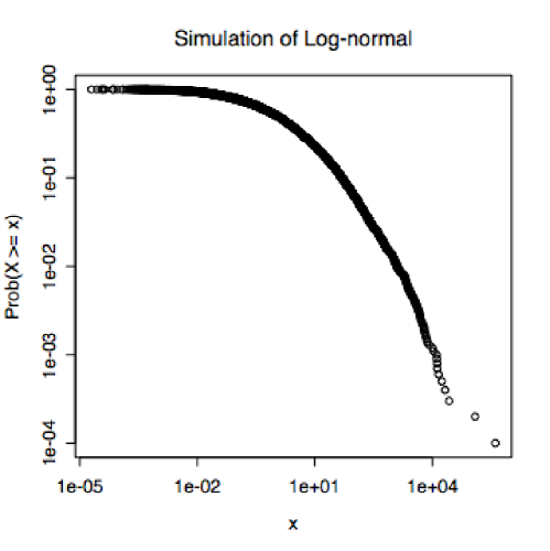
Figure 5: Distribution of 10,000 random numbers, generated according to a log-normal distribution with $\mathbf{E}\left[\log{X}\right]=0$ and $\sigma(\log{X})=3$.

Restricting attention to the “tail” of random numbers $\geq 1$, and doing a usual least-squares fit, gives the line shown in Figure 6.

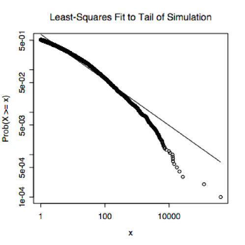
Figure 6: Inability of linear regression on log-log plots to correctly identify power law distributions. Simulation data (circles) and resulting least-squares fit (line) for the 5,112 points in Figure 5 for which $x\geq 1$. The $R^{2}$ of the regression line is 0.962.

One might hope that it would be easy to tell that this data does not come from a power law, since there are a rather large number of observations (5,112), extending over a wide domain (more than four orders of magnitude). Nonetheless, $R^{2}$ is 0.962. This, in and of itself, constitutes a demonstration that getting a high $R^{2}$ is not a reliable indicator that one’s data was generated by a power law.

An Illustration: Blogging

An amusing empirical illustration of the difficulty of distinguishing between power laws and other heavy-tailed distributions is provided by political weblogs, or “blogs” — websites run by individuals or small groups providing links and commentary on news, political events, and the writings of other blogs. A rough indication of the prominence of a blog is provided by the number of other blogs linking to it — its in-degree. (For more on network terminology, see Wuchty, Ravasz and Barabási, this volume.) A widely-read essay by Shirky claimed that the distribution of in-degree follows a power law, and used that fact, and the literature on the growth of scale-free networks, to draw a number of conclusions about the social organization of the blogging community [Shirky-power-law]. A more recent paper by Drenzer and Farrell [Drenzer-Farrell], in the course of studying the role played by blogs in general political debate, re-examined the supposed power-law distribution. Using a large population of inter-connected blogs, they found a definitely heavy-tailed distribution which, on a log-log plot, was quite noticeably concave (7); nonetheless, $R^{2}$ for the conventional regression line was 0.898.

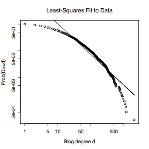
Figure 7: Empirical distribution of the in-degrees of political weblogs (“blogs”). Horizontal axis: number of incoming links $d$; vertical axis: fraction of all blogs with at least that many links, $\mathrm{Pr}(D\geq d)$; both axes are on a log-log scale. Circles show the actual distribution; the straight line is a least-squares fit to these values. This does not produce a properly normalized probability distribution but it does have an $R^{2}$ of 0.898, despite the clear concavity of the curve.

Maximum likelihood fitting of a power law distribution gave $\alpha=-1.30\pm 0.006$, with a negative log-likelihood of $18481.51$. Similarly fitting a log-normal distribution gave $\mathbf{E}\left[\log{X}\right]=2.60\pm 0.02$ and $\sigma(\log{X})=1.48\pm 0.02$, with a negative log-likelihood of 17,218.22. As one can see from Figure 8, the log-normal provides a very good fit to almost all of the data, whereas even the best fitting power-law distribution is not very good at all.

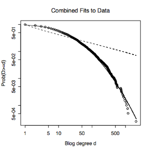
Figure 8: Maximum likelihood fits of log-normal (solid line) and power law (dashed line) distributions to the data from Figure 7 (circles); axes as in that figure. Note the extremely tight fit of the log-normal over the whole range of the curve, and the general failure of the power-law distribution.

A rigorous application of the logic of error testing [Mayo-error] would now consider the probability of getting at least this good a fit to a log-normal if the data were actually generated by a power law. However, since in this case the data were $e^{18481.51-17218.22}\approx 13$ million times more likely under the log-normal distribution, any sane test would reject the power-law hypothesis.

8.5 Other Measures of Complexity

Considerations of space preclude an adequate discussion of further complexity measures. It will have to suffice to point to some of the leading ones. The thermodynamic depth of Lloyd and Pagels [Lloyd-Pagels] measures the amount of information required to specify a trajectory leading to a final state, and is related both to departure from thermodynamic equilibrium and to retrodiction [TDCS]. Huberman and Hogg [Huberman-and-Hogg], and later Wolpert and Macready [Wolpert-Macready-self-dissimilarity] proposed to measure complexity as the dissimilarity between different levels of a given system, on the grounds that self-similar structures are actually very easy to describe. (Say what one level looks like, and then add that all the rest are the same!) Wolpert and Macready’s measure of self-dissimilarity is, in turn, closely related to a complexity measure proposed by Sporns, Tononi and Edelman [Sporns-Tononi-Edelamn-connectivity-and-complexity, Sporns-Tononi-Edelman-theoretical-neuroanatomy, Sporns-Tononi-in-complexity] for biological networks, which is roughly the amount of information present in higher-order interactions between nodes which is not accounted for by the lower-order interactions. Badii and Politi [Badii-Politi] propose a number of further hierarchical scaling complexities, including one which measures how slowly predictions converge as more information about the past becomes available. Other interesting approaches include the information fluctuation measure of Bates and Shepard [Bates-Shepard-information-fluctuation], and the predictability indices of the “school of Rome” [Predictability].

8.6 Relevance of Complexity Measures

Why measure complexity at all? Suppose you are interested in the patterns of gene expressions in tumor cells and how they differ from those of normal cells. Why should you care if I analyze your data and declare that (say) healthy cells have a more complex expression pattern? Assuming you are not a numerologist, the only reason you should care is if you can learn something from that number — if the complexity I report tells you something about the thermodynamics of the system, how it responds to fluctuations, how easy it is to control, etc. A good complexity measure, in other words, is one which is relevant to many other aspects of the system measured. A bad complexity measure lacks such relevance; a really bad complexity measure would be positively misleading, lumping together things with no real connection or similarity just because they get the same score. My survey here has focused on complexity measures which have some claim to relevance, deliberately avoiding the large number of other measures which lack it [DPF-JPC-why].

9 Guide to Further Reading

9.1 General

There is no systematic or academically-detailed survey of the “patterns” of complex systems, but there are several sound informal discussions: Axelrod and Cohen [Axelrod-Cohen-harnessing], Flake [Flake], Holland [Holland-emergence] and Simon [Simon-artificial]. The book by Simon, in particular, repays careful study.

On the “topics”, the only books I can recommend are the ones by Boccara [Boccara-complex-systems] and Flake [Flake]. The former emphasizes topics from physics, chemistry, population ecology and epidemiology, along with analytical methods, especially from nonlinear dynamics. Some sections will be easier to understand if one is familiar with statistical mechanics at the level of, e.g., [Chandler-modern-stat-mech], but this is not essential. It does not, however, describe any models of adaptation, learning, evolution, etc. Many of those topics are covered in Flake’s book, which however is written at a much lower level of mathematical sophistication.

On foundational issues about complexity, the best available surveys [Badii-Politi, CMPPSS] both neglect the more biological aspects of the area, and assume advanced knowledge of statistical mechanics on the part of their readers.

9.2 Data Mining and Statistical Learning

There are now two excellent introductions to statistical learning and data mining, [Hand-Mannila-Smyth] and [tEoSL]. The former is more interested in computational issues and the initial treatment of data; the latter gives more emphasis to pure statistical aspects. Both are recommended unreservedly. Baldi and Brunak [Baldi-Brunak-bioinfo] introduces machine learning via its applications to bioinformatics, and so may be especially suitable for readers of this book.

For readers seriously interested in understanding the theoretical basis of machine learning, [Kearns-Vazirani] is a good starting point. The work of Vapnik [Vapnik-nature, Vapnik-estimating, Vapnik-theory] is fundamental; the presentation in his [Vapnik-nature] is enlivened by many strong and idiosyncratic opinions, pungently expressed. [Cristianini-Shawe-Taylor] describes the very useful class of models called “support vector machines”, as well as giving an extremely clear exposition of key aspects of statistical learning theory. Those interested in going further will find that most of the relevant literature is still in the form of journals — Machine Learning, Journal of Machine Learning Research (free on-line at www.jmlr.org), Neural Computation — and especially annual conference proceedings — Computational Learning Theory (COLT), International Conference on Machine Learning (ICML), Uncertainty in Artificial Intelligence (UAI), Knowledge Discovery in Databases (KDD), Neural Information Processing Systems (NIPS), and the regional versions of them (EuroCOLT, Pacific KDD, etc.).

Much of what has been said about model selection could equally well have been said about what engineers call system identification, and in fact is said in good modern treatments of that area, of which [Nelles-system-identification] may be particularly recommended.

In many respects, data mining is an extension of exploratory data analysis; the classic work by Tukey [Tukey-EDA] is still worth reading. No discussion of drawing inferences from data would be complete without mentioning the beautiful books by Tufte [Tufte-visual-display, Tufte-envisioning, Tufte-visual-explanations].

9.3 Time Series

Perhaps the best all-around references for the nonlinear dynamics approach are [Kantz-Schreiber] and [Abarbanel-analysis]. The former, in particular, succeeds in integrating standard principles of statistical inference into the nonlinear dynamics method. [Sprott-on-time-series], while less advanced than those two books, is a model of clarity, and contains an integrated primer on chaotic dynamics besides. Ruelle’s little book [Ruelle-Lincei] is much more subtle than it looks, full of deep insights. The SFI proceedings volumes [Casdagli-Eubank, time-series-prediction] are very worthwhile. The journals Physica D, Physical Review E and Chaos often have new developments.

From the statistical wing, one of the best recent textbooks is [Shumway-Stoffer]; there are many, many others. That by Durbin and Koopman [Durbin-Koopman-state-space-methods] is particularly strong on the state-space point of view. The one by [Azencott-Dacunha-Castelle] Azencott and Dacunha-Castelle is admirably clear on both the aims of time series analysis, and the statistical theory underlying classical methods; unfortunately it typography is less easy to read than it should be. [Taniguchi-Kakizawa] provides a comprehensive and up-to-date view of the statistical theory for modern models, including strongly non-linear and non-Gaussian models. While many of the results are directly useful in application, the proofs rely on advanced theoretical statistics, in particular the geometric approach pioneered by the Japanese school of Amari et al. [Amari-Nagaoka], This information geometry has itself been applied by Ay to the study of complex systems [Ay-pragmatic-structuring, Ay-information-geometry-on-complexity].

At the interface between the statistical and the dynamical points of view, there is an interesting conference proceedings [Cutler-Kaplan-nonlinear-dynamics-and-time-series] and a useful book by Tong [Tong-nonlinear-time-series]. Pearson’s book [Pearson-discrete-time-dynamic] on discrete-time models is very good on many important issues related to model selection, and exemplifies the habit of control theorists of cheerful stealing whatever seems helpful.

Filtering

Linear filters are well-described by many textbooks in control theory (e.g. [Stengel-optimal-control]), signal processing, time series analysis (e.g. [Shumway-Stoffer]) and stochastic dynamics (e.g. [Honerkamp-stochastic]).

[Eyink-variational-optimal-estimation] provides a readable introduction to optimal nonlinear estimation, draws interesting analogies to non-equilibrium statistical mechanics and turbulence, and describes a reasonable approximation scheme. [Ahmed-filtering] is an up-to-date textbook, covering both linear and nonlinear methods, and including a concise exposition of the essential parts of stochastic calculus. The website run by R. W. R. Darling, www.nonlinearfiltering.webhop.net, provides a good overview and extensive pointers to the literature.

Symbolic Dynamics and Hidden Markov Models

On symbolic dynamics, formal languages and hidden Markov models generally, see [Badii-Politi]. [Lewis-Papadimitriou-computation] is a good first course on formal languages and automata theory. Charniak is a very readable introduction to grammatical inference. [Lind-Marcus] is an advanced treatment of symbolic dynamics emphasizing applications; by contrast, [Kitchens] focuses on algebraic, pure-mathematical aspects of the subject. [Beck-Schlogl] is good on the stochastic properties of symbolic-dynamical representations. Gershenfeld [Gershenfeld-modeling] gives a good motivating discussion of hidden Markov models, as does Baldi and Brunak [Baldi-Brunak-bioinfo], while [Elliott-et-al-HMM] describes advanced methods related to statistical signal processing. Open-source code for reconstructing causal-state models from state is available from http://bactra.org/CSSR.

9.4 Cellular Automata

General

There is unfortunately no completely satisfactory unified treatment of cellular automata above the recreational. Ilachinski [Ilachinski-discrete] attempts a general survey aimed at readers in the physical sciences, and is fairly satisfactory on purely mathematical aspects, but is more out of date than its year of publication suggests. Chopard and Droz [Chopard-Droz-text] has good material on models of pattern formation missing from Ilachinski, but the English is often choppy. Toffoli and Margolus [Toffoli-Margolus] is inspiring and sound, though cast on a piece of hardware and a programming environment which are sadly no longer supported. Much useful material on CA modeling has appeared in conference proceedings [Farmer-Toffoli-Wolfram-CA-conference, Gutowitz-CA-conference, Cellular-Automata-and-Modeling].

CA as Self-Reproducing Machines

The evolution of CA begins in [von-Neumann-self-reproducing], continues in [Burks-essays], and is brought up to the modern era in [Poundstone-recursive]; the last is a beautiful, thought-provoking and modest book, sadly out of print. The modern era itself opens with [ALife-1].

Mathematical and Automata-Theoretic Aspects

Many of the papers in [Wolfram-CA-and-complexity] are interesting. Ilachinski [Ilachinski-discrete], as mentioned, provides a good survey. The Gutowitz volume [Gutowitz-CA-conference] has good material on this topic, too. [new-constructions-in-CA] is up-to-date.

Lattice gases

[Rothman-Zaleski-text] is a good introduction, [Rivet-Boon-lattice-gas-hydro] somewhat more advanced. The pair of proceedings edited by Doolen [Doolen-lattice-gas-for-pdes, Doolen-lattice-gas-methods] describe many interesting applications, and contain useful survey and pedagogical articles. (There is little overlap between the two volumes.)

9.5 Agent-Based Modeling

There do not seem to be any useful textbooks or monographs on agent-based modeling. The Artificial Life conference proceedings, starting with [ALife-1], were a prime source of inspiration for agent-based modeling, along with the work of Axelrod [Axelrod-evol-of-coop]. [Varela-Bourgine-practice-of-autonomous] is also worth reading. The journal Artificial Life continues to be relevant, along with the From Animals to Animats conference series. Epstein and Axtell’s book [Epstein-Axtell] is in many ways the flagship of the “minimalist” approach to ABMs; while the arguments in its favor (e.g., [Epstein-generative-social-science, Macy-Willer-factors-to-actors]) are often framed in terms of social science, many apply with equal force to biology. [Agents-and-GIS] illustrates how ABMs can be combined with extensive real-world data. Other notable publications on agent-based models include [Kohler-Gumerman-dynamics], spanning social science and evolutionary biology; [Bonabeau-on-morphogenesis] on agent-based models of morphogenesis; and [Camazine-et-al-self-org-in-bio] on biological self-organization.

[Budd-understanding-oop] introduces object-oriented programming and the popular Java programming language at the same time; it also discusses the roots of object-orientation in computer simulation. There are many, many other books on object-oriented programming.

9.6 Evaluating Models of Complex Systems

Honerkamp [Honerkamp-stochastic] is great, but curiously almost unknown. Gershenfeld [Gershenfeld-modeling] is an extraordinary readable encyclopedia of applied mathematics, especially methods which can be used on real data. Gardiner [Gardiner-handbook] is also useful.

Monte Carlo

The old book by Hammersley and Handscomb [Hammersley-Handscomb] is concise, clear, and has no particular prerequisites beyond a working knowledge of calculus and probability. [MEJN-on-Monte-Carlo] and [MacKeown-simulation] are both good introductions for readers with some grasp of statistical mechanics. There are also very nice discussions in [Honerkamp-stochastic, tEoSL, Bremaud-markov-chains]. Beckerman [Beckerman-adaptive] makes Monte Carlo methods the starting point for a fascinating and highly unconventional exploration of statistical mechanics, Markov random fields, synchronization and cooperative computation in neural and perceptual systems.

Experimental design

Bypass the cookbook texts on standard designs, and consult Atkinson and Donev [Atkinson-Donev] directly.

Ecological inference

[King-ecological-inference] is at once a good introduction, and the source of important and practical new methods.

9.7 Information Theory

Information theory appeared in essentially its modern form with Shannon’s classic paper [Shannon-1948], though there had been predecessors in both communications [Hartley-1928] and statistics, notably Fisher (see Kullback [Kullback-info-theory-and-stats] for an exposition of these notions), and similar ideas were developed by Wiener and von Neumann, more or less independently of Shannon [Wiener-cybernetics]. Cover and Thomas [Cover-and-Thomas] is, deservedly, the standard modern textbook and reference; it is highly suitable as an introduction, and handles almost every question most users will, in practice, want to ask. [Gray-entropy] is a more mathematically rigorous treatment, now free on-line. On neural information theory, [Spikes-book] is seminal, well-written, still very valuable, and largely self-contained. On the relationship between physics and information, the best reference is still the volume edited by Zurek [complexity-entropy-physics-of-info], and the thought-provoking paper by Margolus.

9.8 Complexity Measures

The best available survey of complexity measures is that by Badii and Politi [Badii-Politi]; the volume edited by Peliti and Vulpiani [Peliti-Vulpiani], while dated, is still valuable. Edmonds [Edmonds-complexity-bibliography] is an online bibliography, fairly comprehensive through 1997. [CMPPSS] has an extensive literature review.

On Kolmogorov complexity, see Li and Vitanyi [Li-and-Vitanyi-1993]. While the idea of measuring complexity by the length of descriptions is usually credited to the trio of Kolmogorov, Solomonoff and Chaitin, it is implicit in von Neumann’s 1949 lectures on the “Theory and Organization of Complicated Automata” [von-Neumann-self-reproducing, Part I, especially pp. 42–56].

On MDL, see Rissanen’s book [Rissanen-SCiSI], and Grünwald’s lecture notes [Grunwald-tutorial-on-MDL]. Vapnik [Vapnik-nature] argues that when MDL converges on the optimal model, SRM will too, but he assumes independent data.

On statistical complexity and causal states, see [CMPPSS] for a self-contained treatment, and [CRS-thesis] for extensions of the theory.

methods locusts