Punctuated equilibria and $1/f$ noise in a biological coevolution model with individual-based dynamics

Abstract

We present a study by linear stability analysis and large-scale Monte Carlo simulations of a simple model of biological coevolution. Selection is provided through a reproduction probability that contains quenched, random interspecies interactions, while genetic variation is provided through a low mutation rate. Both selection and mutation act on individual organisms. Consistent with some current theories of macroevolutionary dynamics, the model displays intermittent, statistically self-similar behavior with punctuated equilibria. The probability density for the lifetimes of ecological communities is well approximated by a power law with exponent near $-2$, and the corresponding power spectral densities show $1/f$ noise (flicker noise) over several decades. The long-lived communities (quasi-steady states) consist of a relatively small number of mutualistically interacting species, and they are surrounded by a “protection zone” of closely related genotypes that have a very low probability of invading the resident community. The extent of the protection zone affects the stability of the community in a way analogous to the height of the free-energy barrier surrounding a metastable state in a physical system. Measures of biological diversity are on average stationary with no discernible trends, even over our very long simulation runs of approximately $3.4\times 10^{7}$ generations.

I Introduction

Biological evolution offers a number of important, unsolved problems that are well suited for investigation by methods from statistical physics. Many of these can be studied using complex, interacting model systems far from equilibrium DROS01 . Areas that have generated exceptional interest among physicists are those of coevolution and speciation. A large class of coevolution models have been inspired by one introduced by Bak and Sneppen BAK93 , in which species with different levels of “fitness” compete, and the least fit species and those that interact with it are regularly “mutated” and replaced by new species with different, randomly chosen fitness. Models in this class exhibit avalanches of extinctions and appear to evolve towards a self-organized critical state BAK87 ; BAK88 . Although such models may be said to incorporate Darwin’s principle of “survival of the fittest,” they are artificial in the sense that mutation and selection are assumed to act collectively on entire species, rather than on individual members of their populations.

In reality, mutations are changes in the genotypes of individual organisms that are introduced or passed on during reproduction. These changes in the genotype affect the phenotype (physical and behavioral characteristics of the organism and its interactions with other organisms), and it is on the level of the phenotypes of individuals that competition and selection act. A number of evolution models (see, e.g., Ref. DROS01 for a review from a physicist’s point of view) therefore take as their basis a genome in the form of a string of “letters” as in Eigen’s quasi-species model of molecular evolution EIGE71 ; EIGE88 . Depending on the level of the modeling, the letters of the genomic “alphabet” can be a (possibly large) number of alleles at a gene locus, or the four nucleotides of a DNA or RNA sequence BAAK99 . However, the size of the alphabet is not of great importance in principle, and it is common in models to use a binary alphabet with the two letters 0 and 1 (or $\pm 1$) DROS01 ; EIGE71 ; EIGE88 ; BAAK99 .

We believe a fruitful approach to the study of coevolution is one in which selection is provided by interspecies interactions along lines commonly considered in community ecology, while genetic variation is provided by random mutations in the genomes of individual organisms. An early attempt in this direction is the coupled $NK$ model with population dynamics introduced by Kauffman and Johnsen KAUF91 ; KAUF93 , but thus far not many similar models have been studied. Recently, Hall, Christensen, and collaborators HALL02 ; CHRI02 ; COLL03 introduced a model they called the “tangled-nature” model, in which each individual lives in a dynamically evolving “fitness landscape” created by the populations of all the other species. Here we consider a simplified version of this model, in which no individual is allowed to live through more than one reproduction cycle. This restriction to nonoverlapping generations enables us to both study the model in detail by linear stability analysis and to perform very long Monte Carlo simulations of its evolutionary behavior. In short, the model consists of populations of different species, on which selection acts through asexual reproduction rates that depend on the populations of all the other species via a constant, random interaction matrix that allows mutualistic, competitive, and predator/prey relations. In addition to these direct interactions, all individuals interact indirectly through competition for a shared resource. The competition keeps the total population from diverging. Genetic variety is provided by a low mutation rate that acts on the genomes of individual organisms during reproduction, inducing the populations to move through genotype space. The resulting motion is intermittent: long periods of stasis with only minor fluctuations are interrupted by bursts of significant change that is rapid on a macroscopic time scale, reminiscent of what is known in evolutionary biology as punctuated equilibria GOUL77 ; GOUL93 ; NEWM85 . A preliminary report on some aspects of the work reported here is given in Ref. RIKV03A .

The main foci of the present paper are the structure and stability of communities and the statistical properties of the dynamical behavior on very long (“geological”) time scales. The rest of the paper is organized as follows. In Sec. II we describe our model in detail, including the detailed Monte Carlo algorithm used for our simulations. In Sec. III we discuss the properties of the fixed points of the population for the mutation-free version of the model. Many of these properties can be understood analytically within a simple mean-field approach. A full, probabilistic description of our model is also possible, although the mathematics is somewhat involved. In Appendix A we provide, for the sake of completeness, the key equations of this approach. In Sec. IV we give a detailed report on our large-scale Monte Carlo simulations and the numerical results, together with a discussion of their relations to the fossil record and to other theoretical models. Finally, in Sec. V, we summarize our results and give our conclusions and suggestions for future studies.

II Model and algorithm

As mentioned in Sec. I, we use a simplified version of the tangled-nature model introduced by Hall, Christensen, and collaborators HALL02 ; CHRI02 ; COLL03 . It consists of a population of individuals with a genome of $L$ genes, each of which can take one of the two values 0 or 1. Thus, the total number of different genotypes is ${\cal N}_{\rm max}=2^{L}$. We consider each different genotype as a separate species, and we shall in this paper use the two terms interchangeably. This is justified by the idea that in the relatively short genomes we can consider computationally, each binary “gene” actually represents a group of genes in a coarse-grained sense.

In our version of the model, the population evolves in discrete, nonoverlapping generations (as in, e.g., many insects), and the number of individuals of genotype $I$ in generation $t$ is $n_{I}(t)$. The total population is $N_{\rm tot}(t)=\sum_{I}n_{I}(t)$. In each generation, the probability that an individual of genotype $I$ produces a litter of $F$ offspring before it dies is $P_{I}(\{n_{J}(t)\})$, while the probability that it dies without offspring is $1-P_{I}$. Although the fecundity $F$ could be quite complex in reality (e.g., a function of $I$ on the average, but random both in time and for each individual), we here take a simplistic approach and assume it is a constant, independent of $I$ and $t$. The main difference from the model of Refs. HALL02 ; CHRI02 ; COLL03 is that the generations are nonoverlapping in our model, while individuals in the original model may live through several successive reproduction cycles. This simplification facilitates theoretical analysis and enables us to make significantly longer simulations than those reported in Refs. HALL02 ; CHRI02 ; COLL03 . In the “opposite” direction, the earlier model could be generalized to include non-trivial “age structures,” since individuals living through several cycles can be assigned an age, with age-dependent survival and reproductive properties LESL45 ; PIEL69 ; CHAR94 ; PENN95 ; HOWA01 ; ZIA02 ; TUZE01A ; CHOW03A ; CHOW03B .

As in the original model HALL02 ; CHRI02 ; COLL03 , the reproduction probability $P_{I}$ is taken as

$$P_{I}(\{n_{J}(t)\})=\frac{1}{1+\exp\left[-\sum_{J}M_{IJ}n_{J}(t)/N_{\rm tot}(t)+N_{\rm tot}(t)/N_{0}\right]}\;.$$ (1)

Here, the Verhulst factor $N_{0}$ VERH1838 represents an environmental “carrying capacity” that might be due to limitations on shared resources, such as space, light, or water. It prevents the total population from indefinite growth, stabilizing it at $O\left(N_{0}\right)$. The interaction matrix $\bf M$ expresses pair interactions between different species such that the element $M_{IJ}$ gives the effect of the population density of species $J$ on species $I$. Thus, a mutualistic relationship is represented by both $M_{IJ}$ and $M_{JI}$ being positive, while both being negative models a competitive relationship. If they are of opposite signs, we have a predator-prey situation. To concentrate attention on the effects of interspecies interactions, we follow Refs. HALL02 ; CHRI02 ; COLL03 in setting the self-interactions $M_{II}=0$. The offdiagonal elements of $M_{IJ}$ are randomly and uniformly distributed on $[-1,1]$ as in Ref. CHRI02 . The interaction matrix is set up at the beginning of the simulation and is not changed later, a situation that corresponds to quenched disorder in spin-glass models FISC91 . We note that we have not attempted to give $\bf M$ a particularly biologically realistic form. Some possible modifications are discussed in Sec. V.

In this model there is a one-to-one correspondence between genotype (the $I$th specific bit string) and phenotype (the $I$th row and column of $\bf M$). Thus, the phenotype specifies both how the $I$th species influences the other species that are either actually or only potentially present in the community (the $I$th column) and how it is influenced by others (the $I$th row). The reproduction probability $P_{I}$ provides selection of the “most fit” phenotypes according to these “traits” (matrix elements) and the populations of the other species present in the community. The effect (or lack thereof) of a particular trait depends on the community in which the species exists, just as a cheetah’s superior speed is only relevant to survival if fast-moving prey is available.

In each generation, the genomes of the individual offspring organisms are subjected to mutation with probability $\mu/L$ per gene and individual. Mutated offspring are re-assigned to their new genotypes before the start of the next generation. This provides the genetic variability necessary for evolution to proceed.

The analytic form of $P_{I}(\{n_{J}(t)\})$, Eq. (1), is by no means unique. For instance, one could use a “soft dynamic” RIKV02 in which the effects of the interactions and the Verhulst factor factorize in $P_{I}$. Alternatively, one could dispense with the exponential and use linear or bilinear relationships instead, as is most common in population biology MURR89 . Investigations of the effects of such modifications are left for the future.

Our evolution algorithm proceeds in three layers of nested loops.

• Loop over generations $t$.

• Loop over the ${\cal N}(t)$ populated genotypes $I$ in generation $t$.

• Loop of length $n_{I}(t)$ over the individuals of genotype $I$. Each individual produces $F$ offspring for generation $t+1$ with probability $P_{I}(\{n_{J}(t)\})$, or dies without offspring with probability $1-P_{I}$. In either case, no individual survives from generation $t$ to generation $t+1$.

• Loop of length equal to the total number of offspring of genotype $I$ generated in loop 3a, attempting to mutate each gene of each individual offspring with probability $\mu/L$ and moving mutated offspring to their respective new genotypes for generation $t+1$.

III Linear stability analysis

Though neither our model nor the simulations are deterministic, a number of their gross properties can be understood in terms of a mean-field approximation that ignores statistical fluctuations and correlations. The time evolution of the populations is then given by the set of difference equations,

$$n_{I}(t+1)=n_{I}(t)FP_{I}(\{n_{J}(t)\})[1-\mu]+(\mu/L)F\sum_{K(I)}n_{K(I)}(t)P_{K(I)}(\{n_{J}(t)\})+O(\mu^{2})\;,$$ (2)

where $\sum_{K(I)}$ runs over the $L$ genotypes $K(I)$ that differ from $I$ by one single mutation (i.e., the Hamming distance HAMM86 $H_{KI}=1$). The corrections of $O(\mu^{2})$ correspond to multiple mutations in single individuals. Naturally, a full investigation of this equation is highly non-trivial, even in the absence of random noise. In particular, Eq. (2) can be regarded as a logistic map in a $2^{L}$-dimensional space. Logistic maps are known to admit, in general, both fixed points and cycles of non-trivial periods MURR89 . To keep both analysis of simulations and theoretical investigations manageable, we choose parameters in such a way that we can focus our attention on fixed points.

Of course, what we simulate are stochastic processes. However, as long as the mutation rate is well below the error threshold for mutational melt-down DROS01 ; EIGE71 ; EIGE88 ; BAAK99 ; HALL02 ; COLL03 , new successful mutations can become fixed in the population before another successful mutant arises. This results in a separation of time scales between the ecological scale of fluctuations within fixed-point communities and the evolutional scale of the durations of such communities DOEB00 , which are known as quasi-steady states (QSS) or quasi evolutionarily stable strategies (q-ESS) HALL02 ; CHRI02 . By ignoring mutations, we can make some analytical progress and gain some insight into the nature and stability properties of these QSS.

III.1 $\cal N$-species fixed points

A fixed point of Eq. (2), defined by

$$n_{I}^{*}(t+1)=n_{I}^{*}(t)\equiv n_{I}^{*}\,\,,$$ (3)

is characterized by having only $\cal N$ ($\leq 2^{L}$) non-vanishing $n_{I}^{*}$. (Henceforth, an asterisk will signify a quantity as a fixed-point value.) Following Ref. ROBE74 , we denote a fixed point as feasible if $n_{I}^{*}>0$ for all $\cal N$ values of $I$. Corresponding to the coexistence of $\cal N$ genotypes, such a point will be simply referred to as an “$\cal N$-species fixed point.” When mutations are ignored, Eq. (2) reduces to

$$n_{I}(t+1)=n_{I}(t)FP_{I}(\{n_{J}(t)\})\,\,.$$ (4)

Specializing to the form of $P_{I}$ given by Eq. (1), we see that all single-species fixed points are trivially “identical,” with $n_{I}^{*}=N_{\mathrm{tot}}^{*}=N_{0}\ln(F-1)$. This somewhat unrealistic result is just a consequence of our choice of $M_{II}=0$ and can be avoided by lifting this restriction. However, the absence of self-interactions places no restriction on the main purpose of our work – the exploration of the effects of random but time independent interspecies interactions.

Proceeding to the ${\cal N}\geq 2$ cases, the existence of an $\cal N$-species fixed point depends critically on the submatrix $\tilde{\mathbf{M}}$, with matrix elements $M_{IJ}$ in which both $I$ and $J$ are among the $\cal N$ species in question. (We shall use the tilde to emphasize that a quantity corresponds to an $\cal N$-species subspace, rather than to the full, $2^{L}$-dimensional genotype space.) In particular, if $\tilde{\mathbf{M}}$ is non-singular, then a unique fixed point exists, as we show below. On the other hand, singular $\tilde{\mathbf{M}}$’s may result in a variety of “degenerate” cases. We provide just two examples to illustrate the mathematical richness of singular $\tilde{\mathbf{M}}$’s. If all elements vanish, then the behavior in this subspace is highly degenerate, with the total population given again by $N_{\mathrm{tot}}^{*}=N_{0}\ln(F-1)$, regardless of $\cal N$. However, the fractions of each species,

$$\rho_{I}^{*}\equiv n_{I}^{*}/N_{\mathrm{tot}}^{*}\;,$$ (5)

are completely undetermined, an understandable consequence of having dynamically indistinguishable species. Another example of a singular interaction submatrix is $\tilde{\mathbf{M}}=\left(\begin{array}[]{cc}0&m>0\\ 0&0\end{array}\right)$ in an ${\cal N}=2$ subspace. Then, Eq. (4) will drive one of the species to extinction, so that no fixed point with both $n_{I}>0$ (stable or unstable) can exist in this two-dimensional subspace, and the system collapses to ${\cal N}=1$. For the remainder of this article, we shall study analytically only the dynamical behavior of interacting species with nonsingular $\tilde{\mathbf{M}}$’s.

To proceed, we insert Eq. (3) into Eq. (4) and arrive at the $\cal N$ equations

$$FP_{I}(\{n_{J}^{*}\})=1\,\,.$$ (6)

With our choice of $P_{I}$, these lead to

$$\sum_{J}M_{IJ}\rho_{J}^{*}=\frac{N_{\mathrm{tot}}^{*}}{N_{0}}-\ln(F-1)\;.$$ (7)

(The analysis in this section remains valid even if $M_{II}\neq 0$, although $M_{II}=0$ is the case explicitly considered elsewhere in this paper.) Note that the right-hand side of Eq. (7) is independent of $I$. Since $\tilde{\mathbf{M}}$ is non-singular, we define its inverse by $\tilde{\mathbf{W}}$, with elements $\tilde{W}_{IJ}$:

$$\tilde{W}_{IJ}\equiv(\tilde{\mathbf{M}}^{-1})_{IJ}\,\,.$$ (8)

Then Eq. (7) can be inverted to give

$$\rho_{I}^{*}=\left[\frac{N_{\mathrm{tot}}^{*}}{N_{0}}-\ln(F-1)\right]\sum_{J}\tilde{W}_{IJ}\,\,.$$ (9)

The only unknown in this equation, $N_{\mathrm{tot}}^{*}$, can now be found via the normalization condition, $\sum\rho_{I}^{*}=1$, which leads to

$$N_{\mathrm{tot}}^{*}/N_{0}=\ln(F-1)+1/\tilde{\Sigma}\;,$$ (10)

where

$$\tilde{\Sigma}\equiv\sum_{IJ}\tilde{W}_{IJ}\,\,.$$ (11)

Putting these into Eq. (9), we have the explicit form of the fixed-point populations:

$$n_{I}^{*}=N_{0}\left[\ln(F-1)+\frac{1}{\tilde{\Sigma}}\right]\frac{\sum_{J}\tilde{W}_{IJ}}{\tilde{\Sigma}}\;.$$ (12)

Although Eq. (12) appears to provide fixed-point values for any choice of control parameters, we emphasize that it is applicable only for a limited range of $F$ and $\tilde{\mathbf{M}}$. The subtlety lies in its stability properties within the $\cal N$-species subspace. First, we remind the reader that, even in the case of ${\cal N}=1$, there are a variety of behaviors. Solutions may have a stable fixed point with either monotonic or oscillatory decay of small deviations, or they may show bifurcations, period doubling, and chaos MURR89 . In the present study, we are interested in the effects of the interspecies interactions, and we therefore choose to focus on systems with monotonically decaying fluctuations in the noninteracting limit. This means that small fluctuations about the fixed point must decay as $\delta(t+1)/\delta(t)\in\langle 0,1\rangle$. For the single-species and ${\mathbf{M}}={\mathbf{0}}$ cases, this restriction is easily translated to the condition $2<F\lesssim 4.5$ for the fecundity. We use $F=4$ in all of our simulations.

Next, through a straightforward linear stability analysis around the $\cal N$-species fixed point, we obtain a condition that represents decay of all small perturbations, i.e., all the eigenvalues of the matrix

$$\left.\frac{\partial n_{I}(t+1)}{\partial n_{J}(t)}\right|_{\{n_{I}^{*}\}}$$ (13)

must have real parts, lying between $-1$ and 1. Carrying out the differentiation and using Eq. (4) to simplify the result, we find this matrix to be of the form ${\bf 1}+\tilde{\bf\Lambda}$, where $\bf 1$ is the $\cal N$-dimensional unit matrix and the elements of $\tilde{\bf\Lambda}$ are given by

$$\tilde{\Lambda}_{IJ}=\left(1-\frac{1}{F}\right)\rho_{I}^{*}\left(M_{IJ}-\ln(F-1)-2/\tilde{\Sigma}\right)\;.$$ (14)

Our criterion translates to the requirement that all the eigenvalues of $\tilde{\bf\Lambda}$ must have real parts that lie in $\langle-2,0\rangle$. Fixed points with this property will be called “internally stable.” Unfortunately, this criterion cannot be made more explicit. Given $F$ and a set of $M_{IJ}$, $\tilde{\bf\Lambda}$ must be constructed using Eqs. (8)–(11) and diagonalized. The matrix $\tilde{\bf\Lambda}$ is recognized as what is known in ecology as the community matrix MURR89 of the $\cal N$-species fixed point for the discrete-time dynamic defined by Eq. (4).

It has been shown, both numerically GARD70 and analytically MAY72 , that the proportion of large, random matrices for which all eigenvalues have a negative real part vanishes as the proportion of nonzero matrix elements increases. This has been used as an argument that highly connected ecosystems are intrinsically unstable MAY72 , contrary to ecological intuition. However, the matrix that must be studied to determine the internal stability of a fixed point is the community matrix $\tilde{\bf\Lambda}$, which has a complicated relationship to the interaction matrix $\bf M$ and should not be expected to have a simple element distribution. In fact, for some bilinear population dynamics models there is numerical evidence that most feasible fixed points are also internally stable ROBE74 ; GILP75 . However, the relations between connectivity and stability have not yet been fully clarified and are still being discussed ROZD01 ; WILM02 .

Of course, issues of internal stability are somewhat academic for simulations. In practice an internally unstable fixed point could not be observed for more than a brief time, especially since the populations would be driven away from such fixed points by the noise due to both the birth/death process and the mutations.

III.2 Stability against other species

Since mutations are essential for the long-time evolutionary behavior, the “external stability” properties of the fixed-point communities are important. Even if the population corresponds to an internally stable $\cal N$-species fixed point, mutations will generate small populations of “invader” species, i.e., genotypes outside the resident $\cal N$-species community. Denoting such invaders by the subscript $i$ and linearizing Eq. (4) about the $\cal N$-species fixed point, we see that the important quantity is the multiplication rate of the invader species in the limit of vanishing $n_{i}/N_{\rm tot}$,

$$\frac{n_{i}(t+1)}{n_{i}(t)}=\frac{F}{1+(F-1)\exp\left[\left(1-\sum_{JK}M_{iJ}{\tilde{W}}_{JK}\right)/\tilde{\Sigma}\right]}\;.$$ (15)

To obtain this result we exploited Eqs. (10) and (12). Explicitly, the condition for stability against the invader, $n_{i}(t+1)/n_{i}(t)<1$, reduces to the requirement that the argument of the exponential function in Eq. (15) must be positive. We also note that, if $M_{iJ}=0$ for all $J$ in the resident community, then the multiplication rate of the invader equals unity. In population biology the Lyapunov exponent $\ln\left[n_{i}(t+1)/n_{i}(t)\right]$ is known as the invasion fitness of the mutant with respect to the resident community DOEB00 ; METZ92 . From Eq. (15) it becomes clear that the success of an invader depends not only on its direct interactions $M_{iJ}$ with each of the resident species, but also on the interactions between the resident species through the inverse interaction submatrix ${\tilde{W}}_{JK}$.

IV Simulation results

The model described in Sec. II was studied by Monte Carlo simulations with the following parameters: $L=13$, $F=4$, $N_{0}=2000$, and $\mu=10^{-3}$. The random matrix $\bf M$ (with zero diagonal and other elements randomly distributed on $[-1,1]$) was chosen at the beginning of each simulation run and then kept constant for the duration of the run. In this regime both the number of populated species ${\cal N}(t)$ and the total population $N_{\rm tot}(t)\sim N_{0}\ln(F-1)\approx 2200$ are substantially smaller than the number of possible species, ${\cal N}_{\rm max}=2^{L}=8192$. This appears biologically reasonable in view of the enormous number of different possible genotypes in nature. (But see further discussion in Sec.IV.5 and Appendix B.) In a QSS, the average number of mutant offspring of species $I$ in generation $t+1$ is approximately $\mu n_{I}(t)$. Thus, with the mutation rate used here, each of the dominant species will produce of the order of one mutant organism per generation. As shown in Sec. IV.2, during a QSS most of these mutants become extinct after one generation. However, due to the small genome size, the same mutant of a species with a large population will be re-generated repeatedly by mutation from the parent species.

A high-population genotype with its “cloud” of closely related low-population mutants could be considered a quasi-species in the sense of Eigen, with the high-population genotype as the “wildtype” DROS01 ; COLL03 ; EIGE71 ; EIGE88 ; BAAK99 . An alternative interpretation of the model is therefore as one of the coevolution of quasi-species COLL03 , in which the successful invasion of a resident community by a mutant represents a speciation event in the lineage of the parent genotype.

IV.1 General features

Most of our simulations were started with a small population of 100 individuals of a randomly selected single genotype, corresponding to the entry into an empty ecological niche by a small group of identical individuals. However, runs starting from a random number of small populations of different species give essentially the same results. Generally, the initial species are not likely to be stable against mutants, and they usually become extinct within 100 generations. To eliminate any short initial transients, most of the quantitative analyses presented here are based on time series from which the first 4096 generations were removed. The simulated quantities were recorded every 16 generations. This time resolution was chosen to be just larger than the average time it would take for the descendants of a single individual of a mutant genotype $i$ to completely replace a resident genotype $J$ of $N_{0}=2000$ individuals in the case of a maximally aggressive mutant, $M_{iJ}=+1$ and $M_{Ji}=-1$. This time, which is obtained by numerical solution of Eq. (15), is about 15 generations and represents a “minimum growth time” for the model. Sampling at shorter intervals would mostly add random noise to the results, while sampling on a much coarser scale could miss important evolutionary events. It is easy to show, by solving Eq. (15) analytically for short times, that the growth time and thus the optimal sampling interval increases logarithmically with $N_{0}$. Most quantitative results in this paper are based on averages over 16 independent simulation runs of $2^{25}=33\,554\,432$ generations each COMP .

We define the diversity of the population as the number of species with significant populations, thus excluding small populations of mainly unsuccessful mutants of the major genotypes. Operationally we define the diversity as $D(t)=\exp\left[S\left(\{n_{I}(t)\}\right)\right]$, where $S$ is the information-theoretical entropy SHAN48 ; SHAN49 ,

$$S\left(\{n_{I}(t)\}\right)=-\sum_{\{I|\rho_{I}(t)>0\}}\rho_{I}(t)\ln\rho_{I}(t)$$ (16)

with

$$\rho_{I}(t)=n_{I}(t)/N_{\rm tot}(t)\;.$$ (17)

This measure of diversity is known in ecology as the Shannon-Wiener index KREB89 . It is different from the definition of diversity as the number of populated species (known in ecology as the species richness KREB89 ) that was used in Refs. HALL02 ; CHRI02 . The entropy-based measure significantly reduces the noise during QSS, caused by unsuccessful mutations.

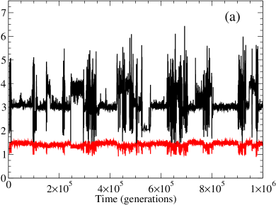
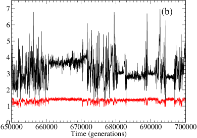
Figure 1: (Color online.) Time series from a simulation of $10^{6}$ generations. The model parameters, which are the same in the subsequent figures, are: mutation rate $\mu=10^{-3}$ per individual, carrying capacity $N_{0}=2000$, fecundity $F=4$, and genome length $L=13$. Top curve (black): Shannon-Wiener diversity index $D(t)=\exp[S(\{n_{I}(t)\})]$. Bottom curve (gray, red online): normalized total population $N_{\rm tot}(t)/[N_{0}\ln(F-1)]$. (a) The whole time series, showing intervals of quasi-steady states (QSS) separated by periods of high activity. (b) Part of one of the periods of high activity, shown on a time scale expanded twenty times. Several shorter QSS are resolved between bursts of high activity. Comparison with (a) suggests statistical self-similarity. See discussion in Secs. IV.1 and IV.3.

The Shannon-Wiener diversity index is shown in Fig. 1(a) for a simulation of $10^{6}$ generations, together with the normalized total population, $N_{\rm tot}(t)/[N_{0}\ln(F-1)]$. We see quiet periods during which $D(t)$ is constant except for small fluctuations, separated by periods during which it fluctuates wildly. The total population $N_{\rm tot}(t)$ is enhanced relative to its noninteracting fixed-point value during the quiet periods, while it decreases toward the vicinity of this value during the active periods.

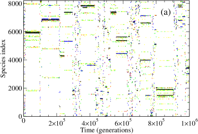
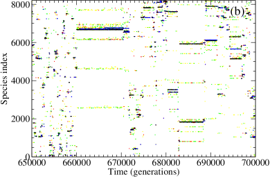
Figure 2: (Color online.) Genotype label $I$ versus time for the same simulation run shown in Fig. 1. In order of decreasing darkness from black to very light gray the symbols indicate $n_{I}\geq 1001$, $n_{I}\in[101,1000]$, $n_{I}\in[11,100]$, $n_{i}\in[2,10]$, and $n_{I}=1$. (Online the colors are black, blue, red, green, and yellow in the same order.) Note that the difference between the label for two species bears no simple relation to their Hamming distance. Each QSS is composed of a different set of species, punctuated by periods during which the population moves rapidly through genotype space. (a) Corresponding to Fig. 1(a), sampled every 960 generations to facilitate plotting. (b) Corresponding to Fig. 1(b), sampled every 48 generations. See discussion in Secs. IV.1 and IV.3.

To verify that different quiet periods indeed correspond to different resident communities $\{n_{I}\}$, we show in Fig. 2 the genotype labels $I$ (integers between 0 and $2^{L}-1$, corresponding to the decimal representation of the genotype bit string) versus time for the populated species. The populations of the different species are indicated by the grayscale (by color online). We see that, in general, the community is completely rearranged during the active periods, so that the quiet periods can be identified with the QSS of the ecology. An exception is afforded by the event near $t=1.5\times 10^{5}$ generations in Figs. 1(a) and 2(a). In this instance the populations of the dominant species decrease, and the total population is for a brief time spread over a larger number of species. However, the dominant species “regain their footing,” and the original resident community continues for approximately another 50 000 generations. This situation is reminiscent of rare events in nucleation theory RIKV94 , in which a fluctuation of the order of a critical or even a supercritical droplet nevertheless may decay back to the metastable state.

IV.2 Stability of communities against invaders

To investigate the stability properties of individual communities against invaders, we chose from a particular simulation run of $10^{6}$ generations ten different QSS of durations longer than 20 000 generations. The genotype labels and fixed-point populations that characterize these QSS are given in the first four columns of Table 1. The population-weighted average of the Hamming distances $H_{IJ}$ between pairs of genotypes in the community,

$$\langle{H}\rangle=\sum_{I}\sum_{J>I}\rho_{I}\rho_{J}\left(\frac{1}{1-\rho_{I}}+\frac{1}{1-\rho_{J}}\right)H_{IJ}\;,$$ (18)

and the corresponding standard deviation,

$$\sigma_{H}=\sqrt{\frac{\cal N}{{\cal N}-1}\sum_{I}\sum_{J>I}\rho_{I}\rho_{J}\left(\frac{1}{1-\rho_{I}}+\frac{1}{1-\rho_{J}}\right)\left(H_{IJ}-\langle H\rangle\right)^{2}},$$ (19)

are shown in the fifth and sixth column, respectively. Even though the community as a whole moves far through the $2^{L}$-dimensional population space, the different QSS communities are seen to retain the property that they consist of relatively close relatives (which of course are all descendants of the single, initial genotype). In Sec. IV.5 we demonstrate that $\langle H\rangle$ and $\sigma_{H}$ remain in the range shown in Table 1, even during very long simulations.

The averages and standard deviations of the offdiagonal interaction-matrix elements ${M}_{IJ}$ between the community members are shown in the seventh and eighth column of Table 1, respectively. They show that the QSS communities are strongly mutualistic, as was also observed for the stable states in Ref. KAUF91 . In contrast, the matrix elements of 22 feasible, but otherwise randomly chosen, communities FEAS ; TREG79 were found to be approximately uniformly distributed on $[-1,1]$.

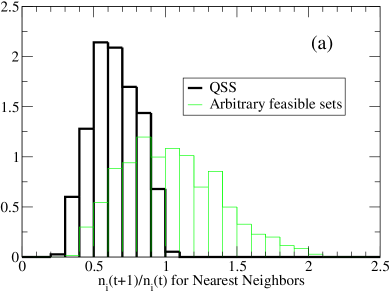
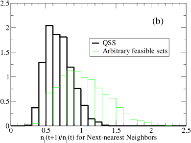
Figure 3: (Color online.) Histograms of the multiplication rate (exponential of the invasion fitness) for mutant species $i$ against each of ten specific QSS (thick, black lines), compared with the same quantity against randomly chosen, feasible communities [thin, gray lines (green on line)]. The multiplication rates are calculated from Eq. (15). (a) When the mutant species differ from the resident community by a Hamming distance of one (nearest neighbors ENDNOTE ). (b) When the mutant species differ from the resident community by a Hamming distance of two (next-nearest neighbors). See discussion in Sec. IV.2.

In Fig. 3 we show histograms of the multiplication rates Eq. (15) (i.e., the exponential function of the invasion fitness) of mutants that differ from the resident species by one single mutation (nearest-neighbor species, $\min_{J}H_{iJ}=1$), and by two mutations (next-nearest-neighbor species, $\min_{J}H_{iJ}=2$) ENDNOTE . Only a very small proportion of the nearest-neighbor mutants have a multiplication rate above unity [Fig. 3(a)]. (In our sample, this very small proportion came from just one of the ten QSS considered.) Among the next-nearest neighbors, on the other hand, a not insignificant proportion may be successful invaders [Fig. 3(b)]. The picture for third-nearest neighbors (not shown) is essentially the same as for the next-nearest neighbors. We also considered the multiplication rates for neighbors of the two most long-lived QSS observed in our simulations, which lasted about $1.0\times 10^{7}$ and $1.4\times 10^{7}$ generations, respectively. They both had no nearest neighbors with multiplication rates above unity, and the proportions for second-and third-neighbors were significantly smaller than those included in Fig. 3. In both parts of Fig. 3 are also shown the multiplication rates for neighbors of the 22 randomly chosen, feasible communities introduced in the previous paragraph. In that case, approximately half of the neighbors at any Hamming distance have multiplication rates above unity.

Summarizing the results from Table 1 and Fig. 3, we see that a long-lived QSS community is characterized by strongly mutualistic interactions and is surrounded by a “protection zone” of closely related genotypes that are very unlikely to successfully invade the resident community. The evidence from the two most long-lived QSS indicates that the average lifetime of a QSS is positively correlated with the extent of the protection zone. By contrast, a randomly chosen, feasible community has an approximately uniform distribution of ${M}_{IJ}$ over $[-1,1]$. It also typically has no protection zone and so is more vulnerable to invasion than a QSS. It is clear from the fact that none of our randomly chosen feasible communities turned out to be a QSS that QSS are relatively rare in this model, even among feasible communities. We believe this may be a favorable condition for continuing evolution, as the ecology can move rapidly from QSS to QSS through series of unstable communities.

IV.3 QSS lifetime statistics

The protection zone surrounding a QSS community acts much like the free-energy barrier that separates a metastable state in a physical system from the stable state or other metastable states. In both cases a sequence of improbable mutations or fluctuations is required to reach a critical state that will lead to major rearrangement of the system. It is thus natural to investigate in detail the lifetime statistics of individual QSS in the way common in the study of metastable decay RIKV94 ; RIKV94A . To this effect we started simulations from each of the ten QSS communities discussed in Sec. IV.2 and ran until the overlap function with the initial community,

$${\cal O}(0,t)=\frac{\sum_{I}n_{I}(0)n_{I}(t)}{\sqrt{\sum_{I}n_{I}(0)^{2}\sum_{J}n_{J}(t)^{2}}}\;,$$ (20)

became less than 0.5, at which time the system was considered to have escaped from the initial state. (We note that the overlap function defined here is simply the cosine of the angle between two unit vectors in the space of population vectors $\{n_{I}\}$.) The precise value of the cutoff used is not important, as long as it is low enough to exclude fluctuations during the QSS RIKV94A . The composition of the population at this time (the “exit community”) was then recorded and the run terminated. Each individual initial QSS was simulated for 300 independent escapes. The means and standard deviations of the individual lifetime distributions are shown in the last two columns of Table 1. The mean lifetimes were found to range over about one order of magnitude, from approximately 10 000 to 80 000 generations. In most cases the individual lifetime distributions were exponential (for which the standard deviation equals the mean), or they had an exponential component that described the behavior in the short-time end of the range of observed lifetimes. In about half of the QSS studied, a tail of very long lifetimes beyond the exponential part (indicated by a standard deviation significantly larger than the mean) was also observed. We further found that an initial QSS does not always escape via the same exit community. Typically, the genotypes in the exit community that are not present in the initial QSS differ from those in the original community by a Hamming distance of two or three. This picture is quite consistent with the stability properties of the QSS discussed in Sec. IV.2.

The range of the lifetimes of the ten QSS discussed above was limited: for a period to be identified by eye as a QSS, its lifetime could not be too short, while the lifetimes were bounded above by the length of the simulation run. The variation of a factor of ten within these limits indicates that the dynamical behavior of the system may display a very wide range of time scales. Another indication to this effect is provided by the details of the activity within periods that appear as high-activity in Figs. 1(a) and 2(a). Such detail is shown in Figs. 1(b) and 2(b). Statistically, the picture in these expanded figures is similar to the one seen on the larger scale, with shorter quiet periods punctuated by even shorter bursts of activity. These observations, which are similar to Refs. HALL02 ; CHRI02 , suggest statistical self-similarity at least over some range of time scales. Indications of self similarity have also been seen in fossil diversity records SOLE97 .

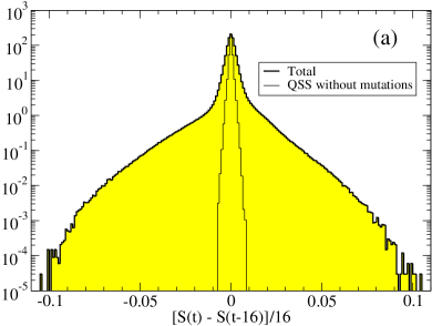
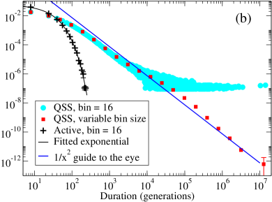
Figure 4: (Color online.) (a) Normalized histogram of entropy changes, averaged over 16 generations (thick curve with shading). Based on 16 independent runs of $2^{25}=33\,554\,432$ generations each. The near-Gaussian central peak corresponds to the QSS, while the near-exponential wings correspond to the active periods. Also shown by a thin line is a histogram based on birth/death fluctuations in ten specific QSS communities with zero mutation rate. The latter is re-normalized so that the maxima of the two histograms coincide. Based on these histograms, a cutoff of $[S(t)-S(t-16)]/16=0.015$ was used to distinguish between active periods and QSS. (b) Normalized histograms for the length of active periods ($\bf+$) and QSS [solid, light gray circles (cyan online) and solid, dark gray squares (red online)]. Based on 16 independent runs of $2^{25}$ generations each. Two of the histograms ($+$ and circles) use a constant bin width of 16 generations. In order to capture the information for large durations, the data for the QSS were also analyzed with exponentially increasing bin size (squares). Error bars showing standard error based on the spread between the individual runs are shown only where they are larger than the symbol size. The black curve through the points for the active periods is a least-squares fit of an exponential distribution to the data. The straight line is a guide to the eye, corresponding to $1/x^{2}$ behavior for the QSS data. See Sec. IV.3 for details.

The suggestion of self-similarity that emerges from Figs. 1 and 2 makes it natural to investigate the statistics of the durations of active periods and QSS over a wider range of time scales than that represented by the ten QSS included in Table 1. From Fig. 1 we see that a reasonable method to make this distinction is to observe the magnitude of the entropy changes, $|dS(t)/dt|$, and to consider the system to be in the active state if this quantity is above some suitably chosen cutoff. This cutoff can best be determined from a histogram of $dS/dt$, such as shown in Fig. 4(a). It shows that the probability density of the entropy derivative consists of two additive parts: a near-Gaussian one corresponding to population fluctuations caused mostly by the birth/death process in the QSS, and a second one corresponding to large changes during the active periods. From this figure we chose the cutoff as 0.015, which was used to classify every sampled time point as either active or quiet. Normalized histograms for the durations of the active and quiet periods are shown in Fig. 4(b). About 97.4% of the time is spent in QSS. The active periods are seen to be relatively short, and their probability density is fitted well by an exponential distribution NOTEa . On the other hand, the lifetimes of the QSS show a very broad distribution CHRI02 – possibly a power law with an exponent near $-$2 for durations longer than about 200 generations. We note that there is some evidence of power laws with exponents near $-$2 in the distributions of several quantities extracted from the fossil record, such as the life spans of genera or families, and the sizes of extinctions SOLE96 ; NEWM96 ; SHIM02 ; SHIM03 . However, the fossil data are sparse and extend over no more than one or two decades in time, and they can be fitted almost as well by exponential distributions SOLE96 . Although our data extend over a much wider range of time scales than the paleontological data, indisputable evidence of a power law remains to be established. Though a few QSS of the order of one million generations will certainly appear in every run of $2^{25}$ generations, more definite conclusions about the statistics of such long QSS must await simulations an order of magnitude longer. Another feature in Fig. 4(b) is that the distribution of QSS durations changes to a smaller slope below about 200 generations. A similar effect has been observed in the fossil record of lifetimes of families SHIM02 ; SHIM03 .

IV.4 Power spectral densities

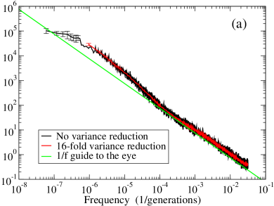
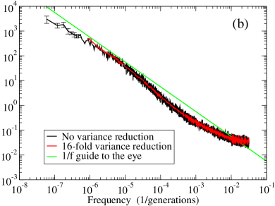
Figure 5: (Color online.) Power spectral densities (PSD) PSD for simulations of length $2^{25}$ generations, sampled every 16 generations and averaged over 16 independent runs. Black curve: no variance reduction. Gray curve (red online): 16-fold variance reduction. Error bars shown for the eight lowest frequencies in each curve are standard errors, based on the spread between the individual runs. The straight line is a guide to the eye, corresponding to $1/f$ behavior. (a) Shannon-Wiener diversity index $D(t)=\exp[S(\{n_{I}(t)\})]$. (b) Normalized total population $N_{\rm tot}(t)/[N_{0}\ln(F-1)]$. See discussion in Sec. IV.4.

From the discussion in Sec. IV.3 it is clear that by using a cutoff for the intensity of some variable which is large in the QSS and small in the active periods (but in both cases with fluctuations of unknown distribution), it is impossible to classify the periods unambiguously. For example, by increasing the cutoff one can make appear as a single QSS period what previously appeared as two successive, shorter QSS periods separated by a short active period. Since the probability of encountering an extremely large fluctuation in a QSS increases proportionally to the length of the QSS, this effect will affect the longest periods most severely. The problem with determining a suitable cutoff can be avoided by, instead of concentrating on period statistics, calculating the power spectral density (PSD) PSD ; PRES92 of variables such as the Shannon-Wiener diversity index or the total population. PSDs for these two quantities are shown in Fig. 5. The PSD for the diversity $D(t)$, shown in Fig. 5(a), appears inversely proportional to the frequency $f$ ($1/f$ noise or flicker noise MILO02 ) for $f>10^{-4}$, goes through a crossover regime of about one decade in $f$ where it is $\sim f^{-\alpha}$ with $\alpha>1$, and then appears to return to $\alpha\approx 1$ for $10^{-6}<f<10^{-5}$. For $f<10^{-6}$ our data are insufficient to determine the PSD unambiguously, and much longer simulations would be necessary NOTEb . In the PSD for $N_{\rm tot}(t)$, shown in Fig. 5(b), the substantial population fluctuations due to the birth/death process during the QSS periods produce a large noise background which interferes with the interpretation at high frequencies. However, for $f<10^{-5}$ the behavior is also consistent with $1/f$ noise.

On time scales much longer than the mean duration of an active period, the time series for the diversity can be approximated by constants during the QSS, interrupted by delta-function like spikes corresponding to the active periods (see Fig. 1). In this limit, the relation between a very wide distribution of the QSS durations $\tau$, described by a long-time power-law dependence of the probability density $p(\tau)\sim\tau^{-\beta}$, and the low-frequency behavior of the PSD is known analytically PROC83 :

$$P(f)\sim\left\{\begin{array}[]{lll}f^{-(\beta-1)}&\mbox{for}&\beta<2\\ 1/\left(f|\ln f|^{2}\right)&\mbox{for}&\beta=2\\ f^{-(\beta-1)(3-\beta)}&\mbox{for}&2<\beta<3\\ |\ln f|&\mbox{for}&\beta=3\\ {\rm const.}&\mbox{for}&\beta>3\end{array}\right.$$

Thus, the approximate $1/f$ behavior of the PSDs in Fig. 5 is consistent with the approximate $1/\tau^{2}$ behavior of the probability density for the QSS durations, shown in Fig. 4(b).

As well as power-law distributions, PSDs that go as $1/f^{\alpha}$ with $\alpha\approx 1$ have been extracted from the fossil record SOLE97 . However, such observed PSDs extend only over one to two decades in frequency (corresponding to power-law probability densities extending only over one or two decades in time), and more recent work indicates that the $1/f$ spectra obtained in Ref. SOLE97 may be artifacts of the analysis method NEWM99 . Although $1/f$ noise, at least in some frequency interval, is a property of our model and is possibly also seen in other models of macroevolution BAK93 (but see Refs. DAER96 ; DAVI01 for conflicting opinions on its presence in the Bak-Sneppen model), whether or not it is really present in the fossil record remains an open question.

IV.5 Stationarity and effects of finite genome size

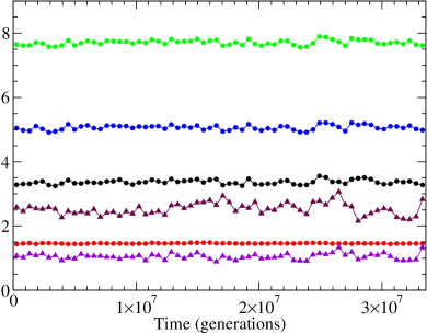
Figure 6: (Color online.) Combined time-window and ensemble averages of various diversity-related measures. Each data point represents an average over a time window of $2^{19}=524\,288$ generations and over 16 (circles) or seven (triangles) independent runs of $2^{25}$ generations each. Shown are, from above to below, the total number of species ${\cal N}(t)$, the number ${\cal N}_{2}(t)$ of species with $n_{I}\geq 2$, the Shannon-Wiener index $D(t)$, the average Hamming distance $\langle H\rangle$ between genotypes in the community, the normalized total population $N_{\rm tot}(t)/[N_{0}\ln(F-1)]$, and the standard deviation $\sigma_{H}$ of the Hamming distances. These data indicate the absence of any systematic long-time trends in the dynamical behavior. See discussion in Sec. IV.5.

An important issue in evolutionary biology is whether or not the evolving ecosystem is stationary in a statistical sense. In Fig. 6 we show several diversity-related measures, averaged over a moving time window and independent simulation runs. These quantities are: the species richness ${\cal N}(t)$, the number ${\cal N}_{2}(t)$ of genotypes with $n_{I}\geq 2$, the Shannon-Wiener index $D(t)$, the total population $N_{\rm tot}(t)$, and the average Hamming distance $\langle H\rangle$ between genotypes in the community and its standard deviation $\sigma_{H}$. As seen in the figure, none of these quantities show any signs of a long-time trend over $2^{25}$ generations. This is consistent with fossil evidence for constant diversity MAYN89 . However, it is in disagreement with simulations of the original version of the tangled-nature model HALL02 , in which a slow growth in species richness was observed. This discrepancy might possibly result from the different forms of the interaction matrix used in the two studies, but it may also be due to the relatively short time series used in Ref. HALL02 .

For our model, a simple, combinatorial phase-space argument (containing neither the individual population sizes nor the mutation rate) indicates that the most probable number of major genotypes should indeed be limited. The argument goes as follows. A community of $\cal N$ genotypes can be chosen in $2^{L}\choose{\cal N}$ different ways and is influenced by ${\cal N}({\cal N}-1)/2$ different pairs of $M_{IJ}$ and $M_{JI}$. We let the probability that the pair of interactions is suitable to forming a stable community be $q$ (if the requirement is simply that both $M_{IJ}$ and $M_{JI}$ should be positive, then $q=1/4$ with our choice of $\bf M$). Thus, a stable $\cal N$-species community can be formed in approximately

$$\Omega({\cal N})={2^{L}\choose{\cal N}}q^{{\cal N}({\cal N}-1)/2}$$ (21)

ways, which obeys the recursion relation

$$\Omega({{\cal N}+1})=\frac{2^{L}-{\cal N}}{{\cal N}+1}q^{\cal N}\Omega({\cal N})$$ (22)

with $\Omega(1)=2^{L}$. This recursion relation can either be used to find the most probable value ${\cal N}^{\,{\dagger}}$ numerically, or one can easily obtain an estimate valid for $2^{L}\gg{\cal N}$: ${\cal N}^{\,{\dagger}}\approx L\ln 2/\ln(1/q)$. The value numerically obtained with $q=1/4$ is ${\cal N}^{\,{\dagger}}=6$, but the close correspondence to the results shown in Fig. 6 may be fortuitous since the dependence of ${\cal N}^{\,{\dagger}}$ on $q$ is only logarithmic.

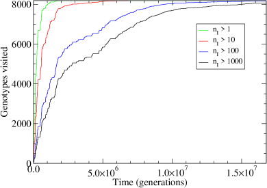
Figure 7: (Color online.) The number of different genotypes visited at different population levels, shown vs time for the first half of a single run of $2^{25}$ generations. From above to below, $n_{I}\geq 2$, $n_{I}\geq 11$, $n_{I}\geq 101$, and $n_{I}\geq 1001$. Horizontal plateaus correspond to QSS. See discussion in Sec. IV.5.

Another question of interest is whether the limited size of the genome leads to “revisiting” of genotypes and communities. The answer is affirmative and indicates the importance of further studies of the effects of the genome size on the long-time dynamical behavior. For genotypes the question of revisits is easy to answer, and the results for a single run of $2^{25}$ generations are shown in Fig. 7. As we see, in less than $3\times 10^{6}$ generations, at least two individuals of every genotype have appeared simultaneously (curve labeled $n_{I}>1$). By the end of the run, almost every genotype has enjoyed being a major species with $n_{I}\geq 1001$ at least once. Plots on a log versus linear scale (not shown) indicate that the curves are reasonably well approximated by exponential approaches to ${\cal N}_{\rm max}$, indicating that genotypes appear to be nearly randomly visited and revisited at a constant rate dependent on $n_{I}$.

For communities, the question is more difficult. If a community is simply defined as an internally stable ${\cal N}$-species community, then an estimate for their total number can be obtained from $\Omega({\cal N})$ of Eq. (21) as described in Appendix B. The result with the parameter values used in this paper is of the order of $10^{12}$. However, unstable communities are also briefly visited, especially during active periods, and a more inclusive way of counting communities would be a coarse-graining procedure based on the overlap function defined in Eq. (20). The nonzero populations are recorded at $t=0$, and the overlap with this initial community is monitored until at some $t^{\prime}>0$ it falls below a suitably chosen cutoff ${\cal O}_{{\rm cut}}$. The set $\{n_{I}(t^{\prime})\}$ is then recorded as a new community with $t^{\prime}$ as its starting time. The process is repeated, now comparing with the newly recorded community. This procedure creates a list of communities and their starting times. To address the issue of revisits, we next scan this list to extract those communities that represent revisits to a previously visited community, or “prototype community.” We compare each community $\{n_{I}(t)\}$ in the original list with the previously found communities $\{n_{I}(\tilde{t})\}$, sequentially in order of increasing $\tilde{t}<t$. If none of the overlaps is greater than ${\cal O}_{{\rm cut}}$, $\{n_{I}(t)\}$ is added to the list of prototypes ${\cal M}_{\rm p}(t_{\rm p})$ with $t_{\rm p}=t$. If an overlap greater than ${\cal O}_{{\rm cut}}$ is found at some $\tilde{t}$, we stop the comparisons and add this community to the list of revisits ${\cal M}_{\rm r}(t_{\rm r})$. The starting time of this revisited community, $t_{\rm r}=t$, is associated in the list ${\cal M}_{\rm r}(t_{\rm r})$ with the unique $t_{\rm p}=\tilde{t}$, the starting time of the associated prototype. As the system evolves, the number of items in each list increases monotonically. Clearly, the cutoffs should be sufficiently small that communities that differ only by fluctuations inside a QSS are not considered different, but sufficiently large to avoid counting significantly different communities as identical. From inspection of the overlap fluctuations in some of the QSS included in Table 1, we found that ${\cal O}_{{\rm cut}}$ in the range of 0.90 to 0.95 is optimal. Estimates of the total numbers of communities (stable and unstable) that can in principle be distinguished by this method are obtained in Appendix B. Depending on details of the assumptions, the estimates vary between $10^{21}$ and $10^{28}$ for these cutoffs.

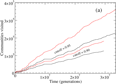
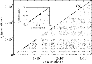
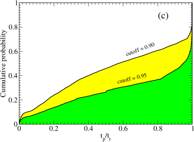
Figure 8: (Color online.) (a) Number of communities visited, shown vs time for a single run of $2^{25}$ generations. A new community is counted whenever the overlap function falls below ${\cal O}_{\rm cut}$. The upper pair of curves corresponds to ${\cal O}_{\rm cut}=0.95$, and the lower pair to 0.90. The top curve in each pair (thin, gray curve, red online) counts both prototype communities and revisits, while the bottom curve (heavy, black curve) excludes revisits. (b) For ${\cal O}_{\rm cut}=0.95$ only, the abscissa $t_{\rm r}$ gives the starting time of each revisit, while the ordinate $t_{\rm p}$ gives the starting time of the associated prototype community. Inset: detail for $t_{\rm p}\lesssim t_{\rm r}$ over $10^{6}$ generations. (c) Lower curve: cumulative histogram for $t_{\rm p}/t_{\rm r}$ from part (b). About 60 % of the revisits are to other recently visited communities, while the rest are approximately uniformly distributed over all previously visited communities. Upper curve: corresponding result for ${\cal O}_{\rm cut}=0.90$. See discussion in Sec. IV.5.

The results of the procedure described above with ${\cal O}_{{\rm cut}}=0.90$ and $0.95$ are shown in Fig. 8 for a single run of $2^{25}$ generations. The upper pair of curves in Fig. 8(a) corresponds to ${\cal O}_{{\rm cut}}=0.95$, and the lower pair to ${\cal O}_{{\rm cut}}=0.90$. In each pair, the upper curve shows the total number of communities in the lists ${\cal M}_{\rm p}\left(t_{\rm p}\right)$ and ${\cal M}_{\rm r}\left(t_{\rm r}\right)$, while the lower curve shows just the number of prototypes in ${\cal M}_{\rm p}\left(t_{\rm p}\right)$. For ${\cal O}_{{\rm cut}}=0.95$, about 40% of the communities are seen to be revisits, while the proportion is about 30% for ${\cal O}_{{\rm cut}}=0.90$. In both cases, the curve for the number of prototypes remains approximately linear, indicating that the supply of previously unvisited communities is nowhere near to being exhausted, even for such a long run. In view of the enormous numbers of available communities estimated above, this result is reasonable. QSS appear as plateaus in the curves showing the numbers of prototypes. Figure 8(b) provides a different perspective (for ${\cal O}_{{\rm cut}}=0.95$ only). Each revisit is represented by a point with $t_{\rm r}$ as abscissa and $t_{\rm p}$ as ordinate. Thus, every point lies strictly below the diagonal. Long-lived QSS appear as large gaps and horizontal segments (e.g., the one near $10^{7}$ generations). The inset shows a detail of $10^{6}$ generations near the diagonal around $1.65\times 10^{7}$. As we see, there are many points just below the diagonal, representing the fluctuations around the (many short-lived) QSS. By contrast, points far below the diagonal represent “throwbacks” to the vicinity of earlier prototype communities. Note that the density of points is much higher just below the diagonal, implying that a large portion of the revisited communities are “fluctuation related.” To highlight these differences, we show the cumulative probability of the ratio $t_{\rm p}/t_{\rm r}$ in Fig. 8(c), in which the lower curve corresponds to the data in Fig. 8(b). For the case of ${\cal O}{{\rm cut}}=0.95$ (lower curve), we see that about 60% of the revisits can be regarded as “fluctuation related” (with $t_{\rm p}\lesssim t_{\rm r}$), while the rest are “throwbacks.” Roughly, the latter component appears to be distributed uniformly over all earlier times. The upper curve shows the corresponding result for ${\cal O}_{{\rm cut}}=0.90$. Corresponding to using a more coarse-grained covering of state space, it naturally displays a larger proportion of throwbacks. Not surprisingly, there is no sharp distinction between these two components of the revisited communities since even a rough partition depends on the details of coarse graining. Nevertheless, we can conclude that the dynamics produces a steady stream of essentially new communities drawn from the vast supply of possibilities.

V Summary and Conclusions

In this work we have studied, by linear stability analysis and large-scale Monte Carlo simulations, a simplified version of the tangled-nature model of biological coevolution, recently introduced by Hall, Christensen, and collaborators HALL02 ; CHRI02 ; COLL03 . Selection is provided by interspecies interactions through the reproduction probability $P_{I}$ [Eq. (1)], which corresponds to a nonlinear population-dynamics model of the community ecology, while the genetic variability necessary for evolution is provided by a low rate of mutations that act on individual organisms during reproduction.

At the low mutation rate studied here, the model provides an intermittent, statistically self-similar behavior, characterized by periods of relative calm, interrupted by bursts of rapid turnover in genotype space. During the quiet periods, or quasi-steady states (QSS), the population consists of a community of a relatively small number of mutualistically interacting genotypes. The populations of the individual genotypes, $n_{I}(t)$, fluctuate near a stable fixed point of a deterministic mean-field, mutation-free version of the model [Eq. (4)]. During the active periods, the system moves through genotype space at a rate that is rapid on a macroscopic (“geological”) time scale, although of course finite on a microscopic (“ecological”) scale. These periods of rapid change are characterized by large fluctuations in the diversity and an overall reduction of the total population. In long simulation runs of $2^{25}$ generations, the ecosystem spends about 97.4% of the time in QSS. The time series produced by the model are statistically stationary, and there is no evidence that any particular quantity is being optimized as the system moves through genotype space. In that sense, the dynamical behavior can probably best be described as a neutral drift DROS01 . Overall, the dynamical behavior of this model resembles closely the punctuated-equilibria mode of evolution, proposed by Gould and Eldredge GOUL77 ; GOUL93 ; NEWM85 .

Investigation of duration statistics for the quiet periods shows a very wide distribution with a power-law like long-time behavior characterized by an exponent near $-2$. Consistent with this result, the power spectral density of the diversity shows $1/f$ noise. While there are claims that similar statistics characterize the fossil record SOLE97 ; SOLE96 ; NEWM96 ; SHIM02 ; SHIM03 , this is still a contested issue SOLE96 ; NEWM99 . At best, observations of power-law distributions and $1/f$ noise in the fossil record extend over no more than one or two decades in time or frequency, and it must remain an open question whether this is the optimal interpretation of the scarce data available.

Due to the absence of sexual reproduction, our model can at best be applied to the evolution of asexual, haploid organisms such as bacteria. It should also be noted that no specific, biologically relevant information has been included in the interaction matrix $\bf M$. In particular, this fact may be responsible for our QSS being strongly dominated by mutualistic relationships. The absence of biologically motivated detail in $\bf M$ is both a strength and a weakness of the model. Its strength lies in reinforcing the notion of universality in macroevolution models, e.g., power law behaviors and $1/f$ noise. By the same token, its weakness lies in the lack of biological detail, to the point that comparison with specific observational or experimental data is difficult. Clearly, the detailed effects of interspecies interactions on the macroevolutionary behavior in models similar to the one studied here represents an important field of future research. Examples include the importance of the connectivity of the interaction matrix, correlated interspecies interactions SEVI04 , and interaction structures corresponding to food webs with distinct trophic levels.

Despite all these caveats, we find it encouraging that such a simple model of coevolution with individual-based dynamics can produce punctuated equilibria, power-law distributions, and $1/f$ noise consistent with current theories of biological macroevolution. We believe future research should proceed in the direction pointed out by this and similar models. This entails combining stochastic models from community ecology with models of mutations and sexual reproduction at the level of individual organisms, and investigating the consequences of more biologically realistic interspecies interactions.

Appendix A Master equation

A complete description of the stochastic process can be given in terms of a master equation, which specifies the evolution of ${\cal P}\left(\vec{n},t\right)$, the probability that the system is found with composition $\vec{n}$ at time $t$. Here, $\vec{n}\equiv\left\{n_{1},n_{2},...,n_{{\cal N}_{\rm max}}\right\}$, and ${\cal N}_{\rm max}=2^{L}$ is the number of individuals of species $I$. In our case, $L=13$ and ${\cal N}_{\rm max}=8192$. Similar to the main text, we define $N_{\rm tot}\equiv\sum_{I}n_{I}$ and let $N_{0}$ be the carrying capacity.

We write the probability for an individual of species $I$ to survive to reproduce as

$$P_{I}\left(\vec{n}\right)=\left\{1+\exp\left[\frac{N_{\rm tot}}{N_{0}}-\sum_{J}M_{IJ}\frac{n_{J}}{N_{\rm tot}}\right]\right\}^{-1}.$$ (23)

The main difference between this expression and Eq. (1) lies in the interpretation. Here, $\vec{n}$ is a “coordinate variable” in the ${\cal N}_{\rm max}$-dimensional space, in contrast to $n_{I}\left(t\right)$ being just a point in this space.

To proceed, we define the symbol ${n_{I}\atopwithdelims[ ]m_{I}}$ as the rate for survival (from $n_{I}$ individuals to $m_{I}$ “mothers”). Since each individual is given a chance to survive according to $P_{I}$, we have

$${n_{I}\atopwithdelims[ ]m_{I}}=\frac{n_{I}!}{m_{I}!\left(n_{I}-m_{I}\right)!}\left(P_{I}\right)^{m_{I}}\left(1-P_{I}\right)^{n_{I}-m_{I}},$$ (24)

which has the form of a binomial distribution. Next, each mother gives rise to $F$ offspring. However, due to mutations, not every offspring is of the same genotype as the mother. Although it is possible to have mutants with a genotype differing from the mother by more than one bit, we restrict ourselves here to a simpler version, namely mutant genotypes that can differ only by one bit. Since our simulations typically involve $\mu\sim 10^{-3}$, this restriction should not lead to serious difficulties. Given that only one bit may be flipped, there are $L+1$ possible varieties of offspring for each maternal genotype. We introduce the notation

$$b_{J,0}\quad\text{for the number of offspring from mother }J\text{ with no mutations}$$

$$b_{J,k}\quad\text{for the number of offspring from mother }J\text{ with the }k\text{th bit flipped}$$

We now define the multinomial-like symbol

$${{Fm_{J}\atopwithdelims[ ]b_{J,0},b_{J,1},...,b_{J,L}}}=\frac{\left(Fm_{J}\right)!}{\left(b_{J,0}\right)!}\left(1-\mu\right)^{b_{J,0}}\prod_{k=1}^{L}\frac{1}{\left(b_{J,k}\right)!}\left(\frac{\mu}{L}\right)^{b_{J,k}},$$ (25)

which is the probability that the $Fm_{J}$ offspring are distributed into the specific set $\left\{b_{J,0},b_{J,1},...,b_{J,L}\right\}$. The last ingredient needed is the connection matrix

$$\Delta_{G}^{J,k}=\left\{\begin{array}[]{cc}1&\text{if genotype }G\text{ is }J\text{ with the }k\text{th bit flipped}\\ 0&\text{otherwise}\end{array}\right.$$ (26)

so that the number of offspring born into species $G$ due to mutations is

$$\tilde{b}_{G}\equiv\sum_{J,k}\Delta_{G}^{J,k}b_{J,k}\;.$$ (27)

The final result is

$${\cal P}\left(\vec{n}^{\,\prime},t+1\right)=\sum_{\vec{n},\vec{m},\left\{b\right\}}\prod_{G}\delta\left(n_{G}^{\prime}-b_{G,0}-\tilde{b}_{G}\right)\prod_{J}{{Fm_{J}\atopwithdelims[ ]b_{J,0},b_{J,1},...,b_{J,L}}}\prod_{I}{{n_{I}\atopwithdelims[ ]m_{I}}}{\cal P}\left(\vec{n},t\right)\;.$$ (28)

In principle, once the dynamics of $\cal P$ is found, the time dependence of various quantities (e.g., averages and correlations) can be computed. For instance,

$$\left\langle n_{I}\right\rangle_{t}\equiv\sum_{\vec{n}}n_{I}{\cal P}\left(\vec{n},t\right)$$ (29)

is the average number of individuals of species $I$ at time $t$. From this very detailed description, we see that the evolution of various quantities can be derived. However, these evolution equations are extremely complex in general and progress is usually possible only by making a “mean-field” approximation, in which all correlations are neglected. Thus, averages of products of $\vec{n}$ are replaced by the products of the averages. As a result, a non-linear evolution equation for $\left\langle\vec{n}\right\rangle_{t}$ results. In a subsequent paper ZIA04 , we shall show that Eq. (2) is precisely the result of such an approach (with $\left\langle\vec{n}\right\rangle_{t}$ denoted by $\{n_{I}\left(t\right)\}$). We shall also demonstrate that, for a QSS, ${\cal P}\left(\vec{n},t\rightarrow\infty\right)$ is well approximated by a Gaussian (for $\mu,1/N_{0}\ll 1$), the center of which is just the fixed point given by Eq. (12). The width of this Gaussian is governed in part by the community matrix $\tilde{{\bf\Lambda}}$ of Eq. (14). In addition to this (systematic, “drift”) part, there is a part governing the noise correlations. Between the two, we can compute distributions of step sizes ($\vec{n}^{\,\prime}-\vec{n}$). For a long-lived QSS, it is easy to compile data so that quantitative comparisons with these predictions can be made.

Appendix B Counting communities

In this Appendix we obtain estimates for the numbers of different communities that could in principle be observed in an infinitely long simulation. Even our most conservative estimate is vastly larger than the numbers observed in a simulation run of $2^{25}$ generations in Sec. IV.5.

If a community is simply defined as an internally stable $\cal N$-species community, then an estimate for their total number can be obtained from $\Omega({\cal N})$ of Eq. (21). Since $\Omega({\cal N})$ is quite sharply peaked around ${\cal N}^{\,{\dagger}}$, we can estimate that $\sum_{\cal N}\Omega({\cal N})\sim\Omega({\cal N}^{\,{\dagger}})\approx 2^{L{\cal N}^{\,{\dagger}}}q^{{\cal N}^{\,{\dagger}}({\cal N}^{\,{\dagger}}-1)/2}\approx\left(2^{a/2}\right)^{aL^{2}}$ with $a=\ln 2/\ln(1/q)$. For $q=1/4$ and $L=13$, this gives $\Omega({\cal N}^{\,{\dagger}})\approx 5.2\times 10^{12}$, while direct summation of $\Omega({\cal N})$ with the same parameters gives $\sum_{\cal N}\Omega({\cal N})=8.5\times 10^{11}$ with 46% due to the contribution from ${\cal N}={\cal N}^{\,{\dagger}}=6$ and convergence by ${\cal N}=11$. As it does not include unstable communities, this would serve as our most conservative estimate of the total number of communities that could be visited in an infinitely long simulation.

To estimate the total number of different communities that can be distinguished by the overlap cutoff method described in Sec. IV.5, we note that the overlap threshold ${\cal O}_{{\rm cut}}$ is simply the cosine of the angle between two vectors in population space, ${\cal O}_{{\rm cut}}=\cos\theta$. For convenience, we define $\epsilon\equiv 1-{\cal O}_{{\rm cut}}$, such that $\epsilon$ is small ($0.1$ and $0.05$). Then, $\theta=\arccos(1-\epsilon)\approx\sqrt{2\epsilon}$. The fact that the number of populated species at any one time is near ${\cal N}^{\dagger}$, means that the direction of the population vector $\{n_{I}\}$ to a reasonable approximation lies within the first hyper-octant of one of ${\cal N}_{\rm tot}\choose{\cal N}^{\dagger}$ ${\cal N}^{\dagger}$-dimensional hyperspheres. The total number of communities that can be distinguished with a cutoff ${\cal O}_{\rm cut}$ is the ratio of the total ${\cal N}^{\dagger}$-dimensional solid angle covered by the hyper-octants to that of a hyper-cone subtended by $\theta$. The solid angle of the hyper-octants is

$$V_{\rm tot}\sim{{\cal N}_{\rm tot}\choose{\cal N}^{\dagger}}\frac{S_{{\cal N}^{\dagger}}}{2^{{\cal N}^{\dagger}}}\;,$$ (30)

where $S_{d}=2\pi^{d/2}/\Gamma(d/2)$ is the surface area of a $d$-dimensional unit sphere. The solid angle of the hyper-cone is

$$C(\epsilon)=S_{{\cal N}^{\dagger}-1}\int_{0}^{\theta}(\sin\beta)^{{\cal N}^{\dagger}-2}\approx S_{{\cal N}^{\dagger}-1}\frac{(2\epsilon)^{({\cal N}^{\dagger}-1)/2}}{{\cal N}^{\dagger}-1}$$ (31)

for small $\epsilon$. Using Stirling’s approximation for the gamma functions in $S_{d}$, $\Gamma(z)\sim(z/e)^{z}\sqrt{2\pi/z}$ and the identity $\lim_{n\rightarrow\infty}\left(1-\frac{1}{n}\right)^{n}=e^{-1}$, we estimate the total number of different communities to be

$$M(\epsilon)\sim{{\cal N}_{\rm max}\choose{\cal N}^{\dagger}}\frac{\sqrt{2\pi{\cal N}^{\dagger}\epsilon}}{(2\epsilon)^{{\cal N}^{\dagger}/2}}\;.$$ (32)

This estimate is reasonable only as long as $\epsilon$ is large enough to exclude minor fluctuations within QSS. Observation of overlap fluctuations in some of the QSS included in Table 1 indicates that ${\cal O}_{\rm cut}$ in the range of 0.90 to 0.95 is optimal. With the parameters used in this work, Eq. (32) yields $M\sim 10^{21}$ for ${\cal O}_{\rm cut}=0.90$ and $M\sim 10^{22}$ for 0.95. If, instead of using ${\cal N}^{\dagger}=6$ we assume that the number of genotypes at any time is near 8, as indicated by the top curve in Fig. 6, these estimates are increased by six orders of magnitude.

Table 1: Composition and lifetime statistics of ten QSS that lasted at least 20 000 generations in a particular simulation run of $10^{6}$ generations. The QSS are listed in order of increasing mean lifetime. Columns one through four give the genotype labels and, in parentheses, the initial populations [the fixed-point populations given by Eq. (12)] for the $\cal N$ genotypes in each QSS. Columns five and six give the population-weighted mean and standard deviation of the ${\cal N}({\cal N}-1)/2$ Hamming distances between the genotypes in the initial community, Eqs. (18) and (19), respectively. Columns seven and eight give the mean and standard deviations of the ${\cal N}({\cal N}-1)$ offdiagonal interaction matrix elements $M_{IJ}$ between the genotypes in the initial community, respectively. Columns nine and ten give the mean and standard deviations of the lifetimes, obtained from 300 independent escapes for each QSS. See discussion in Secs. IV.2 and IV.3.

Initial QSS
Genotype label, $I\;$ (Population, $n_{I}^{*}$)								$\langle{H}\rangle$	$\sigma_{H}$	$\langle M_{IJ}\rangle$	$\sigma_{M_{IJ}}$	$\langle{\rm Lifetime}\rangle$	$\sigma_{\rm Lifetime}$
5180	(1055)	5692	(1506)	7272	(682)			2.79	2.26	0.79	0.16	11 366.2	11 093.4
4251	(1051)	6275	(1077)	6283	(1003)			2.02	1.01	0.70	0.16	12 261.4	11 634.4
2836	(1624)	2982	(1472)					4.00	0.00	0.90	0.06	12 277.7	19 708.3
7135	(995)	7357	(909)	8191	(1201)			3.77	1.96	0.67	0.23	19 289.9	17 865.6
4260	(1212)	4518	(979)	5285	(1078)			1.91	0.99	0.81	0.16	20 216.3	20 056.4
4244	(1034)	6164	(1063)	6196	(330)	6676	(786)	1.99	0.91	0.67	0.30	35 057.9	57 527.9
3334	(915)	3402	(1298)	3403	(1094)			2.45	1.54	0.83	0.13	39 577.2	44 935.3
1122	(1308)	1146	(987)	2149	(1076)			4.50	2.43	0.89	0.07	39 972.4	38 328.8
7380	(1159)	7388	(683)	7412	(1406)			1.28	0.55	0.79	0.16	62 186.5	67 521.7
5860	(671)	7397	(1407)	7653	(473)	7909	(694)	1.95	1.17	0.71	0.25	80 821.8	85 716.1

References

- (1) B. Drossel, Adv. Phys. 50, 209 (2001).
- (2) P. Bak and K. Sneppen, Phys. Rev. Lett. 71, 4083 (1993).
- (3) P. Bak, C. Tang and K. Wiesenfeld, Phys. Rev. Lett. 59, 381 (1987).
- (4) P. Bak, C. Tang and K. Wiesenfeld, Phys. Rev. A 38, 364 (1988).
- (5) M. Eigen, Naturwissenschaften 58, 465 (1971).
- (6) M. Eigen, J. McCaskill, and P. Schuster, J. Phys. Chem. 92, 6881 (1988).
- (7) E. Baake and W. Gabriel, in Annual Reviews of Computational Physics VII, edited by D. Stauffer (World Scientific, Singapore, 2000), p. 203.
- (8) S. A. Kauffman and S. Johnsen, J. theor. Biol. 149, 467 (1991).
- (9) S. A. Kauffman, The origins of order. Self-organization and selection in evolution (Oxford University Press, Oxford, 1993).
- (10) M. Hall, K. Christensen, S. A. di Collobiano, and H. J. Jensen, Phys. Rev. E 66, 011904 (2002).
- (11) K. Christensen, S. A. di Collobiano, M. Hall, and H. J. Jensen, J. theor. Biol. 216, 73 (2002).
- (12) S. A. di Collobiano, K. Christensen, and H. J. Jensen, J. Phys. A 36, 883 (2003).
- (13) S. J. Gould and N. Eldredge, Paleobiology 3, 115 (1977).
- (14) S. J. Gould and N. Eldredge, Nature 366, 223 (1993).
- (15) C. M. Newman, J. E. Cohen, and C. Kipnis, Nature 315, 400 (1985).
- (16) P. A. Rikvold and R. K. P. Zia, in Computer Simulation Studies in Condensed Matter Physics XVI, edited by D. P. Landau, S. P. Lewis, and H.-B. Schüttler (Springer-Verlag, Berlin, in press), e-print arXiv:nlin.AO/0303010.
- (17) P. H. Leslie, Biometrika 33, 183 (1945); Biometrika 35, 213 (1948).
- (18) E. C. Pielou, An Introduction to Mathematical Ecology (Wiley, New York, 1969).
- (19) B. Charlesworth, Evolution in Age-Structured Populations (Cambridge University Press, Cambridge, 1994).
- (20) T. J. Penna, J. Stat. Phys. 78, 1629 (1995).
- (21) M. Howard and R. K. P. Zia, Int. J. Mod. Phys. B 15, 391 (2001).
- (22) R. K. P. Zia and R. J. Astalos, in Computer Simulation Studies in Condensed Matter Physics XIV, edited by D. P. Landau, S. P. Lewis, and H.-B. Schüttler (Springer-Verlag, Berlin, 2002), p. 235.
- (23) D. Chowdhury, D. Stauffer, and A. Kunwar, Phys. Rev. Lett. 90, 068101 (2003).
- (24) D. Chowdhury and D. Stauffer, e-print arXiv:cond-mat/0305322.
- (25) E. Tüzel, V. Sevim, and A. Erzan, Proc. Natl. Acad. Sci. USA 98, 13774 (2001); Phys. Rev. E 64, 061908 (2001).
- (26) P. F. Verhulst, Corres. Math. et Physique 10, 113 (1838).
- (27) K. H. Fischer and J. A. Hertz, Spin Glasses (Cambridge University Press, Cambridge, 1991).
- (28) P. A. Rikvold and M. Kolesik, J. Phys. A 35, L117 (2002).
- (29) J. D. Murray, Mathematical Biology (Springer-Verlag, Berlin, 1989).
- (30) R. W. Hamming, Coding and Information Theory, 2. ed (Prentice-Hall, Englewood Cliffs, 1986).
- (31) M. Doebeli and U. Dieckmann, Am. Naturalist 156, S77 (2000), and references therein.
- (32) A. Roberts, Nature 251, 607 (1974).
- (33) M. R. Gardner and W. R. Ashby, Nature 228, 784 (1970).
- (34) R. M. May, Nature 238, 413 (1972).
- (35) M. E. Gilpin, Nature 254, 137 (1975).
- (36) I. D. Rozdilsky and L. Stone, Ecol. Lett. 4, 397 (2001).
- (37) C. C. Wilmers, S. Sinha, and M. Brede, Oikos 99, 363 (2002).
- (38) J. A. J. Metz, R. M. Nisbet, and S. A. H. Geritz, Trends Ecol. Evol. 7, 198 (1992).
- (39) A single simulation run of generations with the parameters used in this work took about one week on an AMD Athlon PC or about four days on an Intel Xeon PC, in either case running Linux.
- (40) C. E. Shannon, Bell Syst. Tech. J. 27, 379 (1948); Bell Syst. Tech. J. 27, 628 (1948).
- (41) C. E. Shannon and W. Weaver, The Mathematical Theory of Communication (University of Illinois Press, Urbana, 1949).
- (42) C. J. Krebs, Ecological Methodology (Harper & Row, New York, 1989), Chap. 10.
- (43) P. A. Rikvold and B. M. Gorman, in Annual Reviews of Computational Physics I, edited by D. Stauffer (World Scientific, Singapore, 1994), p. 149.
- (44) We constructed the arbitrary, feasible communities by the same method described in Ref. TREG79 : from a larger set of randomly selected genotypes we eliminated those with the most negative until all remaining . The resulting communities have with a mean of 2.5.
- (45) T. Tregonning and A. Roberts, Nature 281, 563 (1979).
- (46) We define an th neighbor of a community of resident species as a genotype that can be created from one or more of the resident genotypes by flipping bits (Hamming distance ), and which is not also a member of the original community or a neighbor of order . If an th neighbor can be created by flipping bits in more than one of the resident genotypes, it is counted with the corresponding multiplicity in the histograms shown in Fig. 3.
- (47) P. A. Rikvold, H. Tomita, S. Miyashita, and S. W. Sides, Phys. Rev. E 49, 5080 (1994).
- (48) R. V. Solé, S. C. Manrubia, M. Benton, and P. Bak, Nature 388, 764 (1997).
- (49) Since the time scale of the durations of the active periods turned out to be so short compared with the sampling interval of 16 generations, only the general shape of the duration distribution marked by in Fig. 4(b) can be taken seriously. In order to resolve the short-time dynamical behavior better, we therefore performed three independent simulations of length generations with sampling every generation. From a histogram of analogous to Fig. 4(a) we determined a cutoff of ( times the cutoff used with sampling every 16 generations). The distribution of active periods was found to be extremely narrow and exponential-like with an average of only about 1.6 generations. The distribution of the QSS durations was not significantly affected by the change in sampling rate.
- (50) R. V. Solé and J. Bascompte, Proc. R. Soc. Lond. B 263, 161 (1996).
- (51) M. E. J. Newman, Proc. R. Soc. Lond. B 263, 1605 (1996).
- (52) T. Shimada, Statistical-Mechanics Study on Diversity, Ph.D. dissertation (The University of Tokyo, Tokyo, 2002).
- (53) T. Shimada, S. Yukawa, and N. Ito, Int. J. Mod. Phys. C (in press).
- (54) The PSD of a variable , where takes discrete values with an increment , is here defined as , where is the average of and with . It was calculated with subroutine spctrm from Ref. PRES92 , using a Welch window and variance reduction as described there.
- (55) W. H. Press, S. A. Teukolsky, W. T. Vetterling, and B. P. Flannery, Numerical Recipes, Second Ed. (Cambridge University Press, Cambridge, 1992).
- (56) E. Milotti, arXiv:physics/0204033 (2002).
- (57) Our simulations with sampling every generation showed, as expected, that the PSD does not have any simple shape for frequencies between the Nyquist frequencies of 1/32, corresponding to sampling every 16 generations, and 1/2, corresponding to sampling every generation.
- (58) I. Procaccia and H. Schuster, Phys. Rev. A 28, 1210 (1983).
- (59) M. E. J. Newman and G. J. Eble, Proc. R. Soc. Lond. B 266, 1267 (1999).
- (60) F. Daerden and C. Vanderzande, Phys. Rev. E 53, 4723 (1996).
- (61) J. Davidsen and N. Lüthje, Phys. Rev. E 63, 063101 (2001).
- (62) J. Maynard Smith, Phil. Trans. R. Soc. Lond. B 325, 241 (1989).
- (63) V. Sevim and P. A. Rikvold, in preparation.
- (64) R. K. P. Zia and P. A. Rikvold, in preparation.