Complexity of Langton’s Ant

Abstract

The virtual ant introduced by C. Langton has an interesting behavior, which has been studied in several contexts. Here we give a construction to calculate any boolean circuit with the trajectory of a single ant. This proves the P-hardness of the system and implies, through the simulation of one dimensional cellular automata and Turing machines, the universality of the ant and the undecidability of some problems associated to it.
Complements and applet at http://www.dim.uchile.cl/ agajardo/langton

1 Introduction

The virtual ant is a system defined by C. Langton [15, 9, 12] on the two-dimensional square lattice: each cell is in one of two states, to-left or to-right. The ant is an arrow between two adjacent cells. It moves one cell forward at each time step, in the direction it is heading. That direction is changed according to the state of the cell where the ant arrives (it turns to the left or to the right); the state of the cell is changed after the ant’s visit. The ant may be seen as a cellular automaton with von Neumann’s neighborhood, or as the head of a two-dimensional Turing machine. Interesting behavior follows: a single ant, starting with all cells in to-left state, has a more or less symmetric trajectory in the first 500 steps; then it goes seemingly randomly for about 10,000 steps, until it suddenly starts building an infinite diagonal “highway” (a periodic motion with drift).

The complex behavior of such a “simple” system motivated several studies, both experimental and analytical, as well as some generalizations and variants. The rule has been generalized to allow more than two states of the cell [1, 4, 6, 10, 11], and to consider several ants [1, 5]. It has also been adapted to different regular lattices [13, 14, 20, 7, 8] and to planar finite graphs [16].

The ant has been studied as a paradigm for signal propagation in random media, in particular as a model of a particle in 2D Lorentz Lattice Gases when the particle interacts with the scatterers that occupy the space and affect its trajectory [14].

1.1 Concepts from Complexity Theory

A decision problem is one where the solution, for a given instance, is yes or no. It is said to be $decidable$ if there is an algorithm which answers the question in a finite time.

Decidable problems are classified in complexity classes, which describe the amount of work needed to solve them. An important class is $P$: problems whose solution can be found in polynomial time. A problem to which any problem in $P$ can be reduced is called $P$-hard; if it also belongs to $P$, is called $P$-complete. Thus, to show that a problem is $P$-hard, it’s enough to reduce a $P$-complete problem to it. Here we say that a problem $A$ is reduced to a problem $B$ (equivalently, that $B$ reduces $A$), if there is a function $R$ computable using a logarithmic amount of space in the size of the input, such that $x$ is a positive instance of $A$ iff $R(x)$ is one of $B$.

We say that a system is $universal$ if it may simulate a universal Turing Machine. This notion of universality implies, in particular, the existence of undecidable problems.

The complexity and undecidability of problems associated to a dynamical system, as well as the existence of some kind of universality in it, are ways to measure the unpredictability of the system. For definitions and results from Complexity Theory, we refer to [17].

1.2 Previous results

There are very few results concerning the dynamics of the ant. The main one says that for any initial configuration, the trajectory of the ant is unbounded. [2]. This has been generalized to the following: the set of cell that are visited infinitely often by the ant (for a given initial configuration) has no corners [19]. A corner of a set is a cell where at least two neighbors are not in the set, and these are not opposite to each other.

Unfortunately, it doesn’t tell us anything else about the behavior of the ant in the long term. The experiments, however, suggest that the long-term behavior of the ant, although unbounded, is unbounded in a highly repetitive way. Specifically, it is conjectured: For any initial configuration with finite support, the ant eventually starts building the periodic highway, in some unobstructed direction. (Here, a configuration is said to have finite support if all but a finite number of cells are in the same state). If the conjecture is true, then any problem associated to the ant, whose input is an initial configuration with finite support, is decidable, for in that case, it suffices to iterate on the configuration until the highway appears. The question may be answered at that point, since the future dynamics is easily predicted.

1.3 Results

We will present a construction that will allow the representation of any boolean circuit as a finite configuration in the lattice. The input variables are represented with the states of certain cells, the calculation of the circuit is performed by the trajectory of a single ant, and the result is written, again, as the states of certain cells. The first consequence of this construction is a lower bound for the complexity of the system:

There exists a problem (“does the ant ever visit this given cell?”) which reduces a $P$-complete problem (the calculation of a boolean circuit) and therefore is $P$-hard.

On the other hand, the construction allows us to simulate any linear cellular automaton for configurations where only a finite number of cells change their states at each time. The consequences are two:

The system is capable of universal computation, since it is able to simulate the dynamics of a universal Turing machine.

There are undecidable problems associated to the behavior of the ant.

2 Construction of circuits

Given any boolean circuit, we’ll show how to build a configuration, where the input variables are represented by states at certain locations, and the result is calculated by the trajectory of a single ant (and is written in a predetermined location). For technical reasons, each of our one-bit input and output registers consist of two horizontally adjacent cells rather than one; this makes it possible for the ant to visit a register without visiting any other nearby cells in that row, and will be seen later to facilitate the re-use of the output register of one logic gate as an input register to a later gate. We construct logical gates with the form described in Figure 1.

At the top of the gate, we have some cells whose states represent the input. At the bottom, some cells represent the output; at the beginning, all output cells are in the to-left state which will represent the logical value false. The ant enters the gate from the left, follows some path inside of the gate, and exits the gate heading to the right. While being in the gate, the ant visits the input cells, and visits (and switches) the correct output cells, according to the function which the gate represents. The changes are done from inside, thus allowing the output cell to be used as the input cell for another gate.

To compute a boolean circuit we just put the input variables in some cells at the top of the configuration (see Figure 2), and for the consecutive stages of evaluation we put consecutive rows of logical gates. The ant will go through every row, starting with the upper one. After going through the last row, the state of the last output cell will contain the evaluation of the circuit for the given input (to change from one row to the next we must construct right-to-left versions of the gates, thus allowing the ant to compute alternate rows in different directions). After that, we assure that the ant will never return to this cell by leading it to a “highway seed” (see Figure 3).

To write a boolean circuit it is enough to have the NOT and the AND functions. To construct the circuit we also use gates that allow us to duplicate, cross and copy variables.

The way to design the gates is represented in Figure 4. Let us describe how the NOT gate works. The ant visits the input cell, and depending on its state the ant will follow different paths. If the input cell is in the to-left state (logical value false), the ant goes to the output cell and changes its state from false to true, and then exits. If the input cell is in the to-right state (logical value true), the ant goes directly to the exit. This is the general scheme of the gates: Some of the allowed trajectories pass through the output register(s) and some do not, before they rejoin. The ant chooses its path through the gate in accordance with the input registers, either passes through the output register(s) (changing the states) or not, and then exits the gate.

Now, let us see how the gates can be embedded in the lattice. Figure 5 shows the configurations for three kinds of crossings (A, B, C), the junction (J), and the paths.

• A: if the ant first enters at 1, it exits at 2. If afterwards it enters at 3, it exits at 4 (see Figure 5).

• B: if the ant first enters at 1, it exits at 2. If afterwards it enters at 3, it exits at 4. But if it enters first at 3, it also exits at 4.

• C: it works as B, but with different relative positions of the input cells.

• J: if the ant enters by 1 or by 2, it exits by 3.

• path: is the configuration that forces the ant to follow a determined trajectory, allowing it to visit the input and the output cells in the required way. A double line with a free extremity may be used as a bent path, since the ant will use both sides, turning around the extrem.

Figures 6, 7 and 8 show the final version of the logical gates.

3 Discussion

The following problem is known to be $P$-complete [18]:

(B) Given a boolean circuit (BC) and a truth assignment. Does the truth assignment satisfy (BC)?

In the previous section we established a function that transforms an instance of (B) into an instance of the following problem:

(P) Given a finite initial configuration of $\mathbf{Z}^{2}$, a given initial position of the ant and a cell $\alpha$. Does the ant ever visit $\alpha$?

Since an instance of (B) is positive if and only if its image in (P) is positive, the transformation is a reduction from (B) to (P). This reduction is polynomial: the number of rows in the gate is bounded by two times the height $(H)$ of the BC plus the number of crossings, i.e., $2(H+W^{2}H)$, where $W$ is the width of the BC. The number of gates in each row is bounded by $W$. That implies that the number of to-right cells ($S$) necessary to simulate an $H\times W$ BC is bounded by $2SWH(W^{2}+1)=o(W^{3}H)$. The algorithm that defines the simulating configuration in $\mathbf{Z}^{2}$ needs only logarithmic space; all it has to do is to read and translate the boolean circuit. For this purpose, it has to memorize numbers such as the position of the symbol that is being translated and the current height of the circuit; these numbers are bounded by the size of the input, and can be recorded in polynomial space. The output of this “drawing” algorithm is the list of coordinates of cells in the to-right state, and is polynomial in the length of the input. This is all we need to legitimate the reduction, and we conclude that (P) is $P$-hard.

In a cellular automata (CA), a quiescent state is defined by the following property: if a cell and all its neighbors are in the quiescent state, the cell remains in it at the next iteration. Hence, all the dynamics of the system takes place at the cells in non-quiescent states and their neighbors. An initial configuration with a finite support (number of non-quiescent states) will keep this property through the iterations of the CA.

Remember that the CA transition rule can be calculated with a multi-output finite boolean circuit. So, for a given linear CA with quiescent state, we can define an initial configuration on the lattice consisting of infinitely many copies of this circuit, arranged in an infinite trapezoidal array with top row of length $L$, as shown in Figure 9. Any initial configuration of the CA whose support has width less than $L$ can be written as the input of the first row, and the ant simulates the CA. For widths bigger than $L$, just put the initial configuration in a lower row, and let the ant start running from the appropriate cell.

It follows that the undecidability of some CA problems is inherited by the ant system. For instance, the problem of knowing whether a given (finite) word $v$ will ever appear in the evolution of a given linear CA, for a given initial configuration with (finite) support $u$, is reduced to the problem of deciding whether a given (finite) block ever appears in the evolution of the ant, for a given (infinite) initial configuration of the lattice. Since a Turing machine can be simulated by a linear CA with quiescent state, the ant is also universal.

4 Conclusions

The construction given here leads us to the following results about the dynamics of a single Langton’s ant:

• The system is $P$-hard, in the sense that it admits a $P$-hard problem. The $P$-hard problem that was shown is associated with initial configurations with finite support.

• The system is capable of universal computation. In spite of being a rather weak notion of universality (which requires an infinite –but finitely described– configuration), it shows that the dynamics of the system is highly unpredictable.

• A direct consequence of the previous point is the existence of undecidable problems. We notice that this result refers to problems associated with initial configurations with infinite support.

There are some open issues related to these results. One of them relates to the complexity; the existence of universal computation suggest that P-hardness is far from being a tight lower bound, and it would be interesting to reduce some $NP$-complete problem to a problem of our system.

On the other hand, the decidability of problems whose input is a configuration with finite support remains an open question. A positive answer would be given if the conjecture stated in 1.2 is found to be true.

Captions of figures

Figure 1: A sketch of a gate. The ant computes the logical gate and changes the states of the output cells. At the beginning the output cells are in the to-left state, representing the logical value false.

Figure 2: The XOR function, built upon AND, NOT, Cross, Copy and Duplicate gates. The ant computes the logical circuit ($\sim(i_{1}\wedge i_{2})\wedge\sim(\sim i_{1}\wedge\sim i_{2})$) row by row. The circuit is satisfied iff the ant visits the output cell, for the given input.

Figure 3: Highway seed. After entering at the indicated point, the ant never crosses the bold lines again, and starts building a highway in the direction of the diagonal arrow. White stands for the to-left state, black for to-right.

Figure 4: A simplified scheme of the gates. The ant follows one of the paths in each gate.

Figure 5: Three kinds of crossings, a junction and a path.

Figure 6: AND and NOT gates.

Figure 7: Cross gate.

Figure 8: Copy and Duplicate gates. The location of the output in the Copy gate can be changed in the horizontal axis, allowing us to fit the positions of the output variables of a row into the inputs of the following row.

Figure 9: The ant simulates each iteration of the CA in a row of gates, crosses the repetitions of the outputs (preparing the next input) and goes to the next row. $R$ stands for the circuit that calculates the rule.

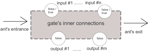
Figure 1:

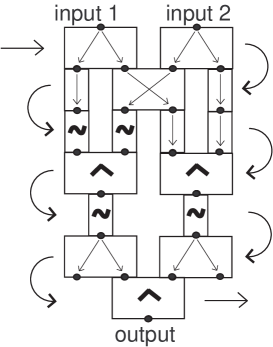
Figure 2:

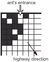
Figure 3:

Copy		NOT		AND

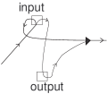
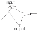
Duplicate		Cross

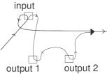
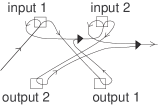
Figure 4:

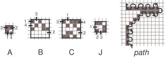
Figure 5:

AND	NOT

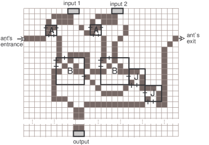
Figure 6:

Cross

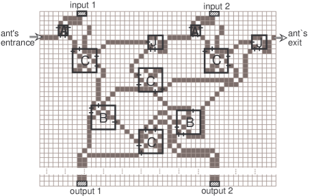
Figure 7:

Copy	Duplicate

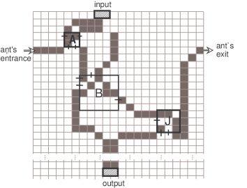
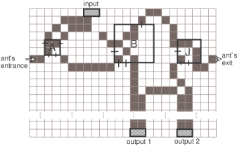
Figure 8:

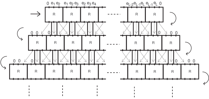
Figure 9:

References

- [1] O. Beuret, M. Tomassini, Behaviour of Multiple Generalized Langton’s Ants, Artificial Life V (1997) 45–50.
- [2] L. Bunimovich, S. Troubetzkoy, Recurrence properties of Lorentz Lattice Gas Cellular Automata, J. of Stat. Physics.67 (1992) 289–302.
- [3] L. Bunimovich, S. Troubetzkoy, Topological dynamics of flipping Lorentz lattice gas models, J. of Stat. Physics.72 (1993) 297–302.
- [4] L. Bunimovich, S. Troubetzkoy, Rotators, periodicity, and absence of diffusion in cyclic cellular automata, J. of Stat. Physics.74 (1994) 1–10.
- [5] B. Chopard, Complexity and Cellular Automata Models, in: S. Ciliberto, T. Dauxois, M. Droz eds., Physics of Complexity, (Editions Frontieres, Gif-sur-Yvette, 1995).
- [6] E. Cohen, New types of diffusion in lattice gas cellular automata, in: M. Mareschal, B. Holian, eds., Microscopic Simulations of Complex Hydrodynamic Phenomena, (Plenum Press, 1992).
- [7] A. Gajardo, E. Goles, Ant’s evolution in a one-dimensional lattice, preprint, 1998.
- [8] A. Gajardo, J. Mazoyer, Langton’s ant on graphs, preprint, 1999.
- [9] D. Gale, The Industrious Ant, The Mathematical Intelligencer.15(2) (1993) 54–58.
- [10] D. Gale, J. Propp, Further Ant-ics, The Mathematical Intelligencer.16(1) (1994) 37–42.
- [11] D. Gale, J. Propp, S. Sutherland, S. Troubetzkoy, Further Travels with my Ant, The Mathematical Intelligencer.17(3) (1995) 48–56.
- [12] D. Gale, Tracking the Automatic ANT and Other Mathematical Explorations (Springer Verlag, N.Y., 1998).
- [13] P. Grosfils, J. P. Boon, E. Cohen, L. Bunimovich, Propagation and organization in a lattice random media, preprint, 1999.
- [14] X. Kong, E. Cohen, Diffusion and propagation in a triangular Lorentz lattice gas cellular automata, J. of Stat. Physics.62 (1991) 737.
- [15] C. Langton, Studying Artificial Life with Cellular Automata, Physica D.22 (1986) 120–149.
- [16] A. Moreira, A. Gajardo, E. Goles, Langton’s ant on planar finite graphs, preprint, 2000.
- [17] C. Papadimitriou, Computational Complexity (Addison-Wesley, 1994).
- [18] M. Sipser, Introduction to the Theory of Computation (PWS Publishing Company, 1996).
- [19] S. Troubetzkoy, Lewis–Parker Lecture 1997 The Ant, Alabama Journal of Mathematics.21(2) (1997).
- [20] F. Wang, Ph.D. dissertation, (The Rockefeller University, 1995).