On the influence of noise on chaos in nearly Hamiltonian systems

Abstract

The simultaneous influence of small damping and white noise on Hamiltonian systems with chaotic motion is studied on the model of periodically kicked rotor. In the region of parameters where damping alone turns the motion into regular, the level of noise that can restore the chaos is studied. This restoration is created by two mechanisms: by fluctuation induced transfer of the phase trajectory to domains of local instability, that can be described by the averaging of the local instability index, and by destabilization of motion within the islands of stability by fluctuation induced parametric modulation of the stability matrix, that can be described by the methods developed in the theory of Anderson localization in one-dimensional systems.

I Introduction

From the point of view of chaotic dynamics, the Hamiltonian systems are marked out by the omnipresence of chaos: for nearly any Hamiltonian system with not less than one and a half degrees of freedom (with the exemption of completely integrable models that are non-robust and therefore exceptionally rare) the chaotic motion is possible for some initial conditions. On the contrary, for the dissipative systems of the same complexity of the structure chaotic motion on strange attractors either could be attained only in limited domains of the parameter space or is inaccessible at all 1 ; 2 .

Inclusion of the dissipative terms, even arbitrarily small, in the canonical equations of motion of the Hamiltonian system can change the character of the motion drastically. In particular, such addition can banish the chaos: for example, for the autonomous Hamiltonian systems with added (viscous) damping the only possible attractors are stable fixed points. It must be noted that this abrupt change may be basically formal, resulting from the presence of the transition to the infinite time limit in the rigorous definitions of important characteristics of chaotic motion, like the Lyapunov exponent and correlators of dynamic variables. In many experimentally relevant models the ratio of the dissipation $\gamma$ to the typical frequency of motion $\omega$ may take very small values. Thus, for radiation damping of vibrations of polyatomic molecules one has $\gamma/\omega\sim 10^{-10}$; the same order of magnitude of $\gamma/\omega$ turns out for the tidal friction of the celestial bodies of the Solar system. In these situations the duration of the ”transient chaos” phase $T\sim\gamma^{-1}$ is so long that accurate determination of characteristics of the chaotic motion can be carried out without the account of dissipation.

Physically the introduction of dissipation in the equations of motion is a form of description of the interaction of an isolated (in the zeroth approximation) system with its environment - a ”heat bath” with practically infinite number of degrees of freedom, continuous spectrum of eigenfrequencies and internal dynamics that is independent of the state of the selected system. This heat bath may be considered also as a source of noise - that is, acting on the selected system random forces, whose statistical characteristics are determined by the properties of the heat bath alone. The problem of simultaneous influence of small dissipation and weak noise on the features of chaotic motion in the originally Hamiltonian non-autonomous system is the main concern of this paper.

The studies of the influence of noise on chaotic motion were pioneered by Lieberman and Lichtenberg 3 just by analysis of the effect of fluctuations on the Hamiltonian non-autonomous system. However, the modern paradigm of the domain was formed later by Crutchfield and Huberman 4 ; 5 who switched the attention to the exploration of strongly dissipative systems (see late review 6 ). The influence of noise on the Hamiltonian systems has been discussed recently in the context of the problem of decay of metastable chaotic states 7 ; 8 , but in general the field doesn’t seem to be fully investigated.

On the contrary, the influence of small dissipation on the Hamiltonian chaos is well understood: Afraimovich, Rabinovich, and Ugodnikov 9 have shown, that with switching on a small dissipation phase trajectories of stable periodic motions of the Hamiltonian non-autonomous systems become attractors with regular motion, and chaos disappears. With the further increase of $\gamma$ these attractors may lose their stability; annihilation of the last one turns the system back into chaotic motion on a strange attractor, that resembles the chaotic motion of the original Hamiltonian system. This pattern needs two specifications. First, the strange attractor may emerge before vanishing of the last of regular ones - the system could be multistable. This case, mentioned in 9 as ”logically possible”, will be met in our model. Secondly, if the Hamiltonian system has no islands of stability that correspond to periodic motion, then the transition from Hamiltonian to dissipative chaos can occur immediately. This case, apparently, will be present in our model too.

The aforesaid permits to specify the main problem of our paper: what intensity of noise is necessary to restore the chaos, repressed by dissipation?

The rest of the text is organized as follows. In Sec. II the basic model is introduced. Sections III and IV treat two mechanisms of restoration of chaos by noise: fluctuation transfer to domains of local instability and parametric destabilization of motion within stability islands. Sec. V treats the influence of strong noise on the Lyapunov exponent and correlation functions of chaotic motion. Sec. VI contains the summary of results and their discussion.

II THE BASIC MODEL

We start from the well-known periodically kicked rotor - the non-autonomous model with the Hamiltonian

$$H\left({I,\theta,t}\right)={{I^{2}}\over 2}+K\cos\theta\sum\limits_{n=-\infty}^{\infty}{\delta\left({t-n}\right)},$$ (1)

where $I$ and $\theta$ are the dynamic variables (canonically conjugated momentum - action and coordinate - angle), $K$ is the control parameter, and $\delta(z)$ is the Dirac delta-function. The stroboscopic mapping that links values of dynamic variables at the moments of time $n-0$ and $n+1-0$, preceding two consequent kicks,

$$I^{\prime}=I+K\sin\theta,\,\,\,\,\,\,\,\,\,\,\,\theta^{\prime}=\theta+I^{\prime},$$ (2)

is known as the standard, or Chirikov - Taylor, mapping and thoroughly studied 10 .

The generalization of the model (1) that includes dissipation and noise will be described by the equation of motion for the angular variable

$$\ddot{\theta}+\gamma\dot{\theta}-K\sin\theta\sum\limits_{n=-\infty}^{\infty}{\delta\left({t-n}\right)=\xi\left(t\right)},$$ (3)

where $\gamma$ is the damping constant. The $\xi(t)$ in the RHS is the Langevin random force, that is a stationary, distributed by a Gaussian law, $\delta$-correlated random process (white noise) with zero mean and the correlator

$$\left\langle{\xi\left(t\right)\xi\left({t+\tau}\right)}\right\rangle=2\gamma\Theta\delta\left(\tau\right),$$ (4)

where $\Theta=k_{B}T$ is the noise temperature in energy units (in the system of scales of the model). The model given by Eqs. (3) and (4) has three parameters: $K,\gamma$ and $\Theta$. We shall restrict ourselves by the domain of small damping, $\gamma\ll 1$, where the system is nearly Hamiltonian.

In the absence of noise, at $\Theta=0$, the stroboscopic mapping for this model is given by equations

$$I^{\prime}=a\left({I+K\sin\theta}\right),\,\,\,\,\,\,\,\,\,\,\,\theta^{\prime}=\theta+b\left({I+K\sin\theta}\right),$$ (5)

where

$$a=e^{-\gamma},\,\,\,\,\,\,\,\,\,\,\,b={\gamma^{-1}({1-e^{-\gamma}})}.$$ (6)

The two-parameter mapping given by Eqs. (5) is a special case of the four-parameter Zaslavsky mapping, that has been introduced in 11 and studied in 12 ; 13 ; 14 . The main efforts of these studies were applied to the case $\gamma\gtrsim 1$. Here we describe in brief the properties of our model for the case of small damping, $\gamma\ll 1$.

At small and moderate values of the control parameter $K$ the most important attractor of the mapping Eqs. (5) is the fixed point $I=0,\theta=\pi$, that is stable in the range

$$K<K_{1}={{2\left({1+a}\right)}\over b}\approx 4\left({1+{7\over{12}}\gamma^{2}}\right).$$ (7)

For $K>K_{1}$ the leading attractor is the symmetric cycle $C^{s}_{2}$ of two points that are related by equations $I^{\prime}=-I,\theta^{\prime}=2\pi-\theta$. It is stable while

$$K<K_{2}={{\pi\left({1+a}\right)}\over b}\approx 2\pi\left({1+{7\over{12}}\gamma^{2}}\right).$$ (8)

For $K>K_{2}$ the leading attractors are two asymmetric cycles of length two $C^{a1}_{2}$ and $C^{a2}_{2}$. The phase coordinates of their points are related by equations $I^{\prime}=-I$, $\theta^{\prime}=\pi+\theta$. They are stable in the domain

$$K<K_{3}={1\over b}\sqrt{\pi^{2}\left({1+a}\right)^{2}+3+a^{2}}$$

$$\approx 2\sqrt{\pi^{2}+1}\left({1+0.152\gamma}\right).$$ (9)

In general case the system defined by Eqs. (5) is multistable. From the first of these equations it follows that the strip

$$\left|I\right|\leq I_{+}={K\over{\exp\gamma-1}}$$ (10)

is the trap (the absorbing set) of the system: any phase trajectory that comes within this strip never leaves it. To determine the comparative roles of basins of attraction of strange and regular attractors of the model the fraction $f$ of chaotic trajectories among the set with random initial conditions, uniformly distributed within the trap, was calculated. The results are presented in Fig. 1.

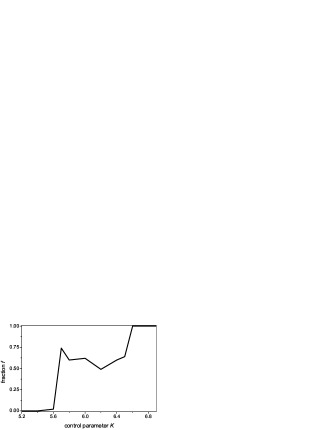
Figure 1: The dependence of the fraction $f$ of the trap area, covered by the basin of attraction of the strange attractor of the system Eqs. (5), on the control parameter $K$. The damping value $\gamma=0.05$. For each value of $K$ 100 uniformly distributed initial conditions was taken.

It can be seen that the strange attractor is born within the domain of stability of the cycle $C^{s}_{2}$, and after the loss of stability of cycles $C^{a1}_{2}$ and $C^{a2}_{2}$, in the range $K>K_{3}(\gamma)$, it remains the only apparent attractor of the system.

For $\Theta>0$ the stroboscopic mapping for the system Eq. (3) has the form

$$I^{\prime} = a\left({I+K\sin\theta}\right)+\upsilon,$$

$$\theta^{\prime} = \theta+b\left({I+K\sin\theta}\right)+\varphi,$$ (11)

where $\upsilon$ and $\varphi$ are the random increments (fluctuations) of action and angle for the unit interval of time. Fluctuations $\upsilon$ and $\varphi$ at the moment of time $t$ after the beginning of the motion with definite initial conditions have the Gaussian distributions with the dispersions

$$D_{\upsilon} = \Theta\left({1-e^{-2\gamma t}}\right),$$

$$D_{\varphi} = {\Theta\over{\gamma^{2}}}\left({2\gamma t-3+4e^{-\gamma t}-e^{-2\gamma t}}\right)$$ (12)

respectively [15]. In our case $\gamma t\equiv\gamma\ll 1$ and the expressions Eqs. (II) could be replaced by their asymptotics

$$D_{\upsilon}=2\gamma\Theta,\,\,\,\,\,\,\,\,\,\,\,\,\,\,\,D_{\varphi}={2\over 3}\gamma\Theta.$$ (13)

Fluctuations $\upsilon$ and $\varphi$ are positively correlated; that has clear physical meaning: positive increment in velocity (that is numerically equal to the action) at the unit interval of time leads, most probably, to the positive increment of coordinate. The correlator $M=\left\langle{\upsilon\varphi}\right\rangle$ by the moment $t$ after the beginning of motion can be calculated by the method described in [15]:

$$M={\Theta\over\gamma}\left({1-e^{-\gamma t}}\right)^{2}.$$ (14)

For $\gamma t\equiv\gamma\ll 1$ the asymptotic value of this correlator is $M=\Theta\gamma$. The joint distribution of fluctuations of action and angle has the form

$$w\left({\upsilon,\varphi}\right)={{\sqrt{3}}\over{2\pi\gamma\Theta}}\exp\left[{-{1\over{\gamma\Theta}}\left({3\varphi^{2}-3\varphi\upsilon+\upsilon^{2}}\right)}\right].$$ (15)

In the presence of noise the phase trajectory can reach any point of the phase space of the system. However, for finite $\gamma$ the system with overwhelming probability will stay in the strip with limited action values that is much narrower than the trap given by Eq. (10). For the description of this domain of concentration of the probability density the term ”attractor” will be used.

III THE THRESHOLD OF CHAOS: TRANSFER TO THE DOMAIN OF LOCAL INSTABILITY

The condition of existence of chaos is, by definition, the positive value of the Lyapunov exponent $\sigma$. Numerical calculation show, that in our model at moderate values of $K\lesssim 5.4$, when the motion of the system in the absence of noise is regular, the Lyapunov exponent increases with $\Theta$ and at some value of $\Theta_{0}$ passes through zero.

We turn to the theoretical description of the onset of chaos. For conservative (area-preserving) mappings with strong chaos rather accurate estimate for the Lyapunov exponent could be obtained by averaging of the local instability index - the logarithm of the maximal in absolute value eigenvalue of the stability matrix - over the domain of chaotic motion 10 ; 16 . Since our model is nearly Hamiltonian, we may try to use this approach.

The stability matrix for the mapping given by Eqs. (II) is

$$A=\left|\begin{matrix}\,\,a&aK\cos\theta\\ \,\,b&{1+bK}\cos\theta\,\ \end{matrix}\right|$$ (16)

The local instability index depends only on the angle $\theta$; for $K<4$

$$\sigma\left(\theta\right)=\ln\left|\,{{S\over 2}+\sqrt{\left({{S\over 2}}\right)^{2}-D}}\,\right|,$$ (17)

where $S=a+1+bK\cos\theta$ is the trace of $A$ and $D=a$ is its determinant. For small $\gamma$ almost everywhere in the interval $\pi/2<\theta<3\pi/2$ the index is negative and constant, $\sigma(\theta)=-\gamma/2$, and the motion is locally stable. Most probably the system stays in this domain, but under the influence of noise it can sporadically enter the domains of local instability. For large enough values of $\Theta$ their contribution can compensate the weak squeezing of phase trajectories in the central part of the attractor.

III.1 Small $K$

For small values $K\ll 1$ in the absence of damping ($\gamma=0$) the evolution of the periodically kicked rotor nearly everywhere in the phase space can be described by the time averaged (and thus time-independent) Hamiltonian of the system, that is given by Eq. (1):

$$\overline{\mathstrut H}\left({I,\theta}\right)=\overline{H\left({I,\theta,t}\right)}={{I^{2}}\over 2}+K\cos\theta.$$ (18)

For an autonomous Hamiltonian system the inclusion of viscous damping and connection to the Langevin (white noise) heat bath lead to the canonical distribution of probability in the phase space

$$W\left({I,\theta}\right)=N\exp\,\,-{{\overline{\mathstrut H}\left({I,\theta}\right)}\over\Theta},$$ (19)

where $N$ is the normalization constant. For the averaging $\sigma=\left\langle{\sigma\left(\theta\right)}\right\rangle$ one needs to know the angular distribution $W(\theta)$. Its normalized form could be found from Eqs. (18) and (19):

$$W\left(\theta\right)={1\over{2\pi I_{0}\left({{K\mathord{\left/{\vphantom{K\Theta}}\right.\kern-1.2pt}\Theta}}\right)}}\exp\,\,-{K\over\Theta}\cos\theta,$$ (20)

where $I_{0}(z)$ is the zeroth order modified Bessel function of the first kind. Since nearly all probability density is concentrated in the stability interval, where $\cos\theta<0$, the contribution of this domain to the averaged value is

$$\sigma_{-}\approx-{\gamma\over 2}.$$ (21)

To calculate the contributions of zones of local instability we neglect the damping; then we have $\sigma\left(\theta\right)\approx\sqrt{K\cos\theta}$. Positive contribution of two instability strips could be estimated by the integral

$$\sigma_{+}\approx{1\over{\pi I_{0}\left({{K\mathord{\left/{\vphantom{K\Theta}}\right.\kern-1.2pt}\Theta}}\right)}}\int\limits_{{{3\pi}/2}}^{2\pi}{\exp\,\,\left({-{K\over\Theta}\cos\theta}\right)}\sqrt{K\cos\theta}\,d\theta.$$ (22)

The threshold values $\Theta_{0}$ found by averaging of the local instability index and by direct numerical calculation are compared in Fig. 2.

Figure 2: The dependence of the temperature threshold of chaos $\Theta_{0}$ on damping $\gamma$ for $K=0.3$. Calculation by Eqs. (21) and (22) (line) and numerical calculation (points).

If $K/\Theta\gg 1$, the integral can be calculated analytically: replacing the Bessel function by its asymptotics for large value of the argument, and approximating the cosine by the linear function, we obtain:

$$\sigma_{+}\approx\sqrt{{1\over{2K}}}\Theta\,\,\exp\,\,-{K\over\Theta}.$$ (23)

From the condition $\left\langle\sigma\right\rangle=\sigma_{-}+\sigma_{+}=0$ the threshold value of temperature is determined by the root of the equation

$$\gamma=\sqrt{{2\over K}}\Theta_{0}\exp\,\,-{K\over\Theta_{0}}.$$ (24)

This expression yields the asymptotic dependence of the temperature threshold of chaos for small $K$: it has the form

$$\Theta_{0}\approx{K\over{\left|{\,\ln\gamma\,}\right|}}$$ (25)

and possesses a logarithmic accuracy.

III.2 Large $K$

The results of the previous subsection shows that for small $K$ the threshold $\Theta_{0}$ grows with the increase of the control parameter $K$, $\Theta_{0}\propto K$. On the other hand, as it was noted in the Sec. II (see Fig. 1), for $K>K_{3}$ chaos in the dissipative system exists (apparently for any initial conditions) even without any noise. For the reasons of continuity we may expect that there may exist a range of values of $K$ where the dependence $\Theta_{0}(K)$ at the constant damping $\gamma$ is decreasing. The numerical calculation confirms this suggestion (see Fig. 3).

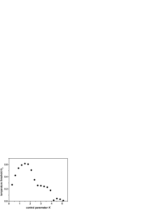
Figure 3: Numerically found dependence of the temperature threshold of chaos $\Theta_{0}$ on the control parameter $K$ for the damping value $\gamma=0.1$.

For the area-preserving mapping Eq. (2), reduced to the basic square $\left({0\leq I<2\pi}\right)\times\left({0\leq\theta<2\pi}\right)$, for large $K$ the chaotic motion takes place in the chaotic component that covers the largest part of the phase space (for $K>2$ the measure of the chaotic component $\mu(K)>0.78$). For the system with damping and noise Eq. (II) we shall retain the name ”chaotic component” for the part of the attractor that includes the points of the chaotic component of the conservative system, and the complementary part will be referred to as ”islands of stability”. Limiting ourselves to the case $K<4$, we will take into account only one island of stability that surrounds the stable fixed point $I=0,\,\theta=\pi$.

Some properties of chaotic motion of the system with damping and noise in the chaotic component could be described by the following simple model. The action variable for one time step receives the increment $\Delta I\approx K\sin\theta$ with the averaged square value $\left\langle{\Delta I^{2}}\right\rangle\approx{{K^{2}}\mathord{\left/{\vphantom{{K^{2}}2}}\right.\kern-1.2pt}2}$. For the motion in the chaotic component the correlations of the consequent values of $\theta$ are small 17 ; 18 , and we can depict the evolution of the system as the motion of the rotor with the damping $\gamma$ under the influence of some Langevin force, a white noise coming from the source with an effective temperature $\Theta^{\star}$. From Eq. (13) we have the estimate $\Theta^{\star}\approx K^{2}/{4\gamma}\gg 1$. In this approximation the distribution of phase density in the chaotic component will become canonical one, with uniform distribution of angles and the Gaussian distribution of action,

$$W_{c}\left({I,\theta}\right)=\sqrt{{\gamma\over{2\pi^{3}K^{2}}}}\exp\,\left({-{{2\gamma}\over{K^{2}}}I^{2}}\right).$$ (26)

This expression is applicable for small $\gamma$ and large $K$.

Let’s assume that in the island of stability the probability density also has the distribution of the canonical form

$$W_{i}\left({I,\theta}\right)=N\exp\,\left({-{{\tilde{H}\left({I,\theta}\right)}\over\Theta}}\right),$$ (27)

where $\tilde{H}(I,\theta)$ is an effective Hamiltonian (a function that is constant on the invariant curves of the standard mapping (2)), and $N$ is the normalization constant. This assumption is plausible in view of Eq. (19); additional support for it will be obtained in the next section.

If $\gamma$ and $\Theta$ are sufficiently small, then the phase trajectory can leave the island of stability or return to it only by passing through the narrow strip of the width $\delta\sim\sqrt{\gamma\Theta}$ along the border of the island of stability. The probability $P$ of finding a phase point in the chaotic component could be found from the balance considerations by equalizing $W_{c}$ and $W_{i}$ on this border. For $P\ll 1$ we can neglect the non-uniformity of the distribution Eq. (26) in action and obtain the estimate

$$P=N\sqrt{{{2\pi^{3}K^{2}}\over\gamma}}\exp\left({-{\Delta\over\Theta}}\right),$$ (28)

where $\Delta$ is the value of the effective Hamiltonian ${\tilde{H}\left({I,\theta}\right)}$ on the border of the island of stability. At present we can not calculate this quantity analytically, but from its value taken from the numerical calculations (and depending only on $K$) by Eq.(28) we can find the dependence of $P$ on $\Theta$ and $\gamma$.

In the numerical experiment the basic square $\left({0\leq I<2\pi}\right)\times\left({0\leq\theta<2\pi}\right)$ has been separated into $10^{4}$ cells. A chaotic trajectory of the standard mapping Eq. (2) in this square was calculated for $10^{5}$ time steps, and all cells, in which the trajectory came at least once, were marked as the mask of the chaotic component. Then for the trajectories of the system with damping and noise Eq.(II) the probability $P$ has been calculated as the fraction of points of the trajectory whose projections on the basic square got into one of the cells of the mask.

The results of numerical calculations for the values $K=3$ and $\gamma=0.05$ are shown in Fig. 4. Fit of the linear dependence of $\ln P$ on the inverse temperature $\beta=\Theta^{-1}$ for these points gives values $\Delta=1.07$ and $N=0.057$.

Figure 4: Dependence of the probability $P$ of finding a trajectory of motion of the system with damping and noise in the place of the chaotic component of the standard mapping on the inverse temperature $\beta=\Theta^{-1}$ for the values $K=3$ and $\gamma=0.05$. Numerical calculation (points) and linear fit to the points (line).

From the assumption that the motion inside the stability island gives to the Lyapunov exponent the negative contribution $\sigma_{-}=-\gamma/2$, and that the positive contribution from the motion in the chaotic component is $\sigma_{+}=\sigma\left(K\right)P$, where $\sigma(K)$ is the Lyapunov exponent value of the Hamiltonian system, for the temperature threshold of chaos we obtain the equation

$$\Theta_{0}={{\Delta\left(K\right)}\over{\ln\left[{\sigma\left(K\right)N\sqrt{{\mathstrut}8\pi^{3}K^{2}\gamma^{-3}}}\right]}}.$$ (29)

The threshold values $\Theta_{0}$ found by calculating the probability of transfer to the chaotic component by this formula and by direct numerical calculation are compared in Fig. 5. From the Eq. (29) it is seen that essentially $\Theta_{0}$ is proportional to the ”activation energy” $\Delta(K)$; the dependence on other parameters is only logarithmic. The general behaviour of the dependence on Fig. 3 could be explained by decrease of the size of the stability island with the increase of $K$; the dip around $K=4$ reflects the restructurization of the regular attractor.

Figure 5: The dependence of the temperature threshold of chaos $\Theta_{0}$ on damping $\gamma$ for $K=3$. Calculation by Eq. (29) (line) and numerical calculation (points).

IV THE THRESHOLD OF CHAOS: PARAMETRIC DESTABILIZATION IN THE ISLANDS OF STABILITY

Although the agreement between the theoretical curve and the numerical points in Fig. 5 is rather convincing, the increase of discrepancy at very small $\gamma$ is strange: just in this domain the damping must have especially little influence, and the picture of transfer between the island of stability and the chaotic component promises to be asymptotically exact. Furthermore, this discrepancies could not be neglected from the quantitative point of view, since for the sharp dependence of $P(\Theta)$ small variations of $\Theta$ at low temperatures produce large changes in the positive contribution to the Lyapunov exponent $\sigma_{+}=\sigma\left(K\right)P$. For example, for $K=3$ and $\gamma=0.01$ substitution of the numerically found value $\Theta_{0}=0.086$ in the Eq. (28) gives $P=2.6\cdot 10^{-5}$ and $\sigma_{+}=1.8\cdot 10^{-5}=3.5\cdot 10^{-3}(\gamma/2)$. Thus we must conclude that there exists another mechanism creating the instability that acts on the parts of phase trajectories that are localized within the islands of stability.

In the domain $2<K<4$, in which the island of stability surrounds the fixed stable point $I=0,\theta=\pi$, we can consider the dynamic variables $x=\theta-\pi$ and $y=I$ to be small. Then by substitution $\cos x\approx 1-x^{2}/2$ the matrix of stability could be represented in the form

$$\tilde{A}=\left|\begin{matrix}\,\,a&{-aK+a\eta\,\,}\\ \,\,b&{1-bK+b\eta}\,\,\end{matrix}\right|,$$ (30)

where $\eta=Kx^{2}/2$ are small corrections. The quantities $\eta$ are fluctuating under the influence of noise and could be treated as random. The stochastic modulation of parameters of the mapping leads to destabilization of the motion. The corresponding exponent of instability $\sigma_{+}$ we will calculate in the conservative approximation, since the contribution to the common Lyapunov exponent from damping $\sigma_{-}=-\gamma/2$ and from stochastic modulation $\sigma_{+}$ for small $\gamma$ are additive.

The transformation of variables determined by matrices Eq. (30) at $\gamma=0$ can be reduced to the three-term recurrent relation for the angular variable:

$$x_{n+1}-\left({2-K-\eta_{n}}\right)x_{n}+x_{n-1}=0.$$ (31)

This expression can be interpreted as an equation for amplitudes $x_{n}$ of the stationary wave function in the quantum one-dimensional tight-binding model with unit non-diagonal matrix elements (transfer integrals) between adjacent sites, random site energies $\eta_{n}$ and the energy eigenvalue $E=2-K$ (one-dimensional chain with diagonal disorder). The calculation of the Lyapunov exponent for this system was carried out in the context of the theory of Anderson localization. For the case in which $\eta_{n}$ are independent random variables with zero mean, $\left\langle\eta\right\rangle=0$, and small dispersion, $\left\langle{\eta^{2}}\right\rangle\ll 1$, the Lyapunov exponent has been calculated by Derrida and Gardner 19 . Correlations between consequent values of $\eta_{n}$ were taken into account by Tessieri and Izrailev 20 . The stochastic Lyapunov exponent is proportional to the dispersion of fluctuating parameter $\eta$:

$$\sigma_{+}={{\left\langle{\eta^{2}}\right\rangle}\over{2\left({4K-K^{2}}\right)}}C\left(\omega\right).$$ (32)

The correlation factor $C(\omega)$ in this expression has the form

$$C\left(\omega\right)=1+2\sum\limits_{k=1}^{\infty}{b_{\eta}\left(k\right)\cos\left({2\omega k}\right)},$$ (33)

where $b_{\eta}(k)$ are normalized correlation functions of the random variable $\eta$, $b_{\eta}\left(k\right)={{\left\langle{\eta_{i}\eta_{i+k}}\right\rangle}\mathord{\left/{\vphantom{{\left\langle{\eta_{i}\eta_{i+k}}\right\rangle}{\left\langle{\eta^{2}}\right\rangle}}}\right.\kern-1.2pt}{\left\langle{\eta^{2}}\right\rangle}}$, and

$$\omega=\arccos{{2-K}\over 2}$$ (34)

is the average angle of rotation of a vector by the linearized standard mapping. Formula Eq. (32) is applicable for the values of $K$ that are not too close to $K=0$ or $K=4$. In our case $\left\langle\eta\right\rangle\neq 0$, but we can include this value in the parameter $K$; this renormalization will change its value into $\tilde{K}=K\left({1-{{\left\langle{x^{2}}\right\rangle}\mathord{\left/{\vphantom{{\left\langle{x^{2}}\right\rangle}2}}\right.\kern-1.2pt}2}}\right)$. In what follows we shall retain the designation $\eta$ for the fluctuating quantity with zero mean, $\eta={{K\left({x^{2}-\left\langle{x^{2}}\right\rangle}\right)}\mathord{\left/{\vphantom{{K\left({x^{2}-\left\langle{x^{2}}\right\rangle}\right)}2}}\right.\kern-1.2pt}2}$. To use the expression Eq. (32) we have to determine statistical characteristics of the variable $\eta$: its dispersion and correlation function. It must be noted at once that for calculation of these quantities the account of damping is essential.

IV.1 Invariant density in the island of stability

Since for low temperatures $\Theta$ the phase trajectory nearly all the time is located in the vicinity of the stable fixed point, for finding the invariant distribution of the probability density $W(x,y)$ we may use the linearized mapping $\hat{L}$,

$$x^{\prime}=by+\left({1-bK}\right)x,\,\,\,\,\,\,y^{\prime}=ay-aKx.$$ (35)

The motion of the system on a unit time interval can be separated into two stages: the first is the evolution under the mapping Eq. (35), the second is addition of the fluctuation increments (cf. Eq. (II)). The probability of coming in the vicinity of the point $(u,v)$ after the first stage is proportional to the value of the invariant density in the vicinity of its prototype $\hat{L}^{-1}\left({u,v}\right)$. The influence of noise can be described by the convolution of the obtained distribution with the distribution of fluctuation increments $w(\upsilon,\varphi)$ Eq. (15). Thus for the invariant density we obtain the following integral equation:

$$W\left({x,y}\right)=a^{-1}{\displaystyle{\int\!\!\!\int}}{du\,dv}\,W\left({u-{\displaystyle{b\over a}}v,{\displaystyle{Ku}+{{1-bK}\over a}}v}\right){\displaystyle{{\sqrt{3}}\over{2\pi\gamma\Theta}}}\exp\left\{{\displaystyle{-{1\over{\gamma\Theta}}}\left[{3\left({u-x}\right)^{2}-3\left({u-x}\right)\left({v-y}\right)+\left({v-y}\right)^{2}}\right]}\right\}.$$ (36)

We will look for its solution in the form of a canonical distribution with the effective Hamiltonian, that is bilinear in action $y$ and angle $x$:

$$W\left({x,y}\right)=\exp\,-{1\over\Theta}\left({Ax^{2}+Bxy+Cy^{2}}\right).$$ (37)

After substitution of this expression in Eq. (36), integration and equivalizing the coefficients at the identical powers of dynamic variables, in the lowest order in $\gamma$ we obtain the parameters of the function Eq. (37):

$$A={3K\over{6-K}},\,\,\,\,\,\,\,B=-{3K\over{6-K}},\,\,\,\,\,\,\,C={3\over{6-K}}.$$ (38)

Now we can calculate the moments of dynamic variables, e.g.

$$\left\langle{x^{2}}\right\rangle={{12-2K}\over{12K-3K^{2}}}\Theta,\,\,\,\,\,\,\,\,\,\,\,\left\langle{xy}\right\rangle={{6-K}\over{12-3K}}\Theta,$$ (39)

and the dispersion of the fluctuating quantity,

$$\left\langle{\eta^{2}}\right\rangle={1\over 2}\left({{{12-2K}\over{12-3K}}}\right)^{2}\Theta^{2},$$ (40)

that enters in the RHS of Eq. (32).

IV.2 Correlation function

With the known form of the invariant density, the correlation function of the angular variable $x$ could be calculated by the direct integration. For the linearized mapping Eq. (35) the values of $B_{x}\left(n\right)=\left\langle{x_{i}x_{i+n}}\right\rangle$ could be expressed through two moments, $\left\langle{x^{2}}\right\rangle$ and $\left\langle{xy}\right\rangle$. For example,

$$\,\,\,\,B_{x}\left(0\right)=\left\langle{x^{2}}\right\rangle\,\,\,\,\,\,\,B_{x}\left(1\right)=\left({1-bK}\right)\left\langle{x^{2}}\right\rangle+b\left\langle{xy}\right\rangle,$$

(41)

$$B_{x}\left(2\right)=\left({1-bK\left({2+a}\right)+b^{2}K^{2}}\right)\left\langle{x^{2}}\right\rangle$$

$$+b\left({a-bK+1}\right)\left\langle{xy{\mathstrut}}\right\rangle.$$ (42)

For small $\gamma$ the normalized correlation function $b_{x}\left(n\right)={{B_{x}\left(n\right)}\mathord{\left/{\vphantom{{B_{x}\left(n\right)}{B_{x}\left(0\right)}}}\right.\kern-1.2pt}{B_{x}\left(0\right)}}$ can be expressed in the form

$$b_{x}\left(n\right)=\cos\left({\tilde{\omega}n}\right)\exp\left({-{\gamma\over 2}n}\right).$$ (43)

Here the tilde over $\omega$ reminds that the renormalized value of $\tilde{K}$ must be used in calculations. This formula is compared to the numerical calculations in Fig. 6.

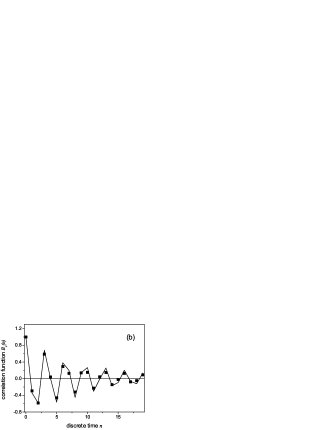
Figure 6: Normalized correlation function $b_{x}(n)$ of the angular variable for the values of parameters $K=3$ and $\gamma=0.2$. (a) For $\Theta=0.05$, (b) for $\Theta=0.2$. Calculation by Eq. (43) (line) and numerical calculation (points).

The normalized correlation function of the fluctuating variable $\eta$ can be calculated in a similar way:

$$b_{\eta}\left(n\right)=\cos^{2}\left({\tilde{\omega}n}\right)\exp\left({-\gamma n}\right).$$ (44)

With this expression one can calculate the correlation factor $C(\omega)$ (see Eq. (33)). For small $\gamma$ it is given by the expression $C\left(\omega\right)\approx\left({2\gamma}\right)^{-1}$. With it from the condition $\sigma_{-}+\sigma_{+}=0$ follows the estimate of the temperature threshold of chaos

$$\Theta_{0}=2\sqrt{4K-K^{2}}{{12-3K}\over{12-2K}}\gamma.$$ (45)

This formula is too crude for the practical application: it gives only the estimate of $\Theta_{0}$ from below. Here is the reason for this limitation: the expressions Eqs. (43) and (44) for the correlation functions are valid only for small temperatures, $\Theta\lesssim\gamma$. For larger values the nonlinear terms that are present in the exact mapping Eq. (II) change the frequency of oscillations of the correlation function $b_{\eta}(n)$ (see Fig. 6(b)); by this they spoil the resonance with the cosine factor under the summation sign in Eq. (33) and considerably decrease the value of $C(\omega)$, down to the value about 2-3 on the threshold of chaos. The numerical calculation shows that around $\Theta_{0}$ the temperature dependence of the Lyapunov exponent is accurately described by the formula

$$\sigma=-{\gamma\over 2}+\kappa\Theta^{2}$$ (46)

with a coefficient $\kappa$ about unity. From Eq. (46) the simple approximation for the temperature threshold follows:

$$\Theta_{0}\approx c\sqrt{\gamma},$$ (47)

where constant $c$ is about unity. The fit of the law Eq. (47) to the points in Fig. 5 gives $c\approx 0.88$.

V STRONG NOISE

In this section we will look at the effects of noise with temperature much higher than the chaos threshold $\Theta_{0}$.

V.1 The Lyapunov exponent

With the increase of the noise temperature the Lyapunov exponent increases monotonously and tends to some finite limit $\sigma_{\infty}$ (see Fig. 7).

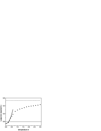
Figure 7: The dependence of the Lyapunov exponent $\sigma$ on the noise temperature $\Theta$ for $K=3$ and $\gamma=0.1$ obtained from numerical calculation (points). Parabola in the left part (solid line) - calculation by Eq. (46) with $\kappa=1$. Horizontal dashed line marks the limiting value $\sigma_{\infty}=0.538$.

Since with the increase of noise the typical values of increments of the angle ($\varphi$) and of the action ($\upsilon$) grow, $\varphi\sim\upsilon\sim\sqrt{{\mathstrut}\gamma\Theta}$ (see Eq. (13)), for $\Theta\gg\gamma^{-1}$ all correlations of dynamical variables vanish. Therefore the limiting value $\sigma_{\infty}$ is equal to the Lyapunov exponent of the infinite product of the matrices Eq. (17) with uncorrelated values of $\theta$, uniformely distributed in the interval $0\leq\theta<2\pi$. For small $K$ the value of $\sigma_{\infty}$ can be calculated from the result of 19 for the localization length at the band edge, namely:

$$\sigma_{\infty}=-{\gamma\over 2}+0.229K^{{2\mathord{\left/{\vphantom{23}}\right.\kern-1.2pt}3}}.$$ (48)

The dependence given by this equation is in good agreement with the numerical data up to the value of $K\approx 1$ (see Fig. 8).

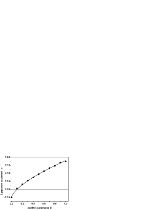
Figure 8: The dependence of the limiting value of the Lyapunov exponent $\sigma_{\infty}$ on the control parameter $K$ for $\gamma=0.1$. Calculation by Eq. (48) (line) and numerical calculation (points).

It may be noted that from Eq. (48) it follows that for a given value of damping $\gamma$ there exist a range of values of the control parameter $K<3.23\,\gamma^{{3\mathord{\left/{\vphantom{32}}\right.\kern-1.2pt}2}}$ in which chaos could not be reached for any intensity of the noise. For large values $K\gtrsim 3$ the limit $\sigma_{\infty}$ does not differ noticeably from the Lyapunov exponent $\sigma(K)$ of the original Hamiltonian system.

V.2 The angular correlations

In the theory of the standard mapping it is customary to study the angular correlations through the properties of the variable $s=\sin\theta$ 17 ; 18 . From the symmetry considerations it has zero mean: $\left\langle s\right\rangle=0$.

Let’s consider the correlation of two consequent values of this variable:

$$B_{s}\left(1\right)=\left\langle{\sin\theta\,\,\sin\theta^{\prime}}\right\rangle.$$ (49)

When the invariant density $W(I,\theta)$ is known, the calculation of the correlation Eq. (49) is reduced to the two-fold integration. For small $K$ the distribution can be taken as the canonical one with the averaged Hamiltonian Eq. (18). With approximating the angular distribution by the Gaussian function, for small damping $\gamma$ we have the expression

$$B_{s}\left(1\right)={1\over 2}\left({1-\exp\left({-{{2\Theta}\over K}}\right)}\right)\exp\left({-{\Theta\over 2}}\right).$$ (50)

It is compared to the numerical data in Fig. 9(a).

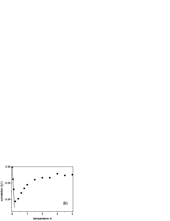
Figure 9: Dependence of the correlation function $B_{s}(1)$ of the angular variable $s=\sin\theta$ on the noise temperature $\Theta$. (a) For $K=0.3$, $\gamma=0.01$. Calculation by Eq. (50) and numerical calculation (points). (b) For $K=3$, $\gamma=0.05$. Calculation by Eq. (51) (line) and numerical calculation (points).

For large values of $K\geq 2$ and small temperatures the value of $B_{s}(1)$ could be calculated from the distribution Eq. (37):

$$B_{s}\left(1\right)=\left({1-K}\right)\left\langle{x^{2}}\right\rangle+\left\langle{{\mathstrut xy}}\right\rangle={{12-8K+K^{2}}\over{12K-3K^{2}}}\Theta.$$ (51)

It is compared to the numerical data in Fig. 9(b). The numerical calculation shows in this case the decrease of $B_{s}(1)$ with $\Theta$ for sufficiently high temperatures. The reason for it is qualitatively clear. We have two competing contributions to $B_{s}(1)$: a negative one from the island of stability and a smaller positive one from the motion in the chaotic component. The increase of the temperature leads to the increase of the probability $P$ of the motion within the chaotic component, that eventually suppresses the negative contribution. The way of accurate calculation of $B_{s}(1)$ for high temperatures at present is not known.

Thence both for small and large values of the control parameter $K$ the increase of the noise temperature (from zero) induces first the increase of the correlation of the consequent values of the angular variable $s=\sin\theta$ up to some maximal value, and then its decrease.

VI CONCLUSION

Above we have studied the model of periodically kicked rotor with added damping and white noise. We expect that some of the established features and relations are typical and will hold at least qualitatively for many representative non-autonomous Hamiltonian systems with chaotic motion. With this in view, in this Section we summarize main results of this paper in a generalized way. Since the growth of the control parameter of the standard mapping $K$ increases both the amount (given by the invariant measure $\mu$ of the chaotic component) and the intensity (given by Lyapunov exponent $\sigma$) of chaos we will refer to $K$ as to the strength of chaos. In what follows (as well as everywhere above) the Lyapunov exponent denotes the largest of the characteristic exponents of the stroboscopic mapping of the system that can take negative as well as positive values (one have to keep in view that for systems - flows with finite phase velocity there is always one zero characteristic Lyapunov exponent that corresponds to evolution of the infinitesimal displacement along the phase trajectory).

1. If chaos in a Hamiltonian system is suppressed by addition of small dissipation, then addition of white noise can, as a rule, restore the chaotic motion. The exception is found only for very weak chaos, when the system remains regular at arbitrarily intense noise (see Sec. V.A). The increase of the noise intensity raises the Lyapunov exponent. In wide context this fact is not quite trivial, since there is an example of the system for which noise diminishes the (positive) Lyapunov exponent, eventually turning it negative 21 .

2. The temperature threshold of chaos depends on the strength of chaos of the Hamiltonian system in a non-monotonous way (see Fig. 3). For weak chaos it increases with the strength (in our model – by linear law, see Eq. (25)), since the effective ”potential well” corresponding to the island of stability becomes deeper, whereas for strong chaos the threshold decreases due to the shrinking of the islands of stability.

3. There are two essentially different mechanisms of the chaotization of motion by noise. The first one is the fluctuational transfer of the motion from the stability island to the locally unstable regions of the phase space; its contribution to the Lyapunov exponent depends on the noise temperature by the ”activation law”, $\sigma_{+}\propto\exp(-\Delta/\Theta)$ (see Eqs. (23) and (28) and Fig. 4). The second is the parametric destabilization inside the islands of stability created by small fluctuations of nonlinear terms of the stroboscopic mapping; its contribution to the Lyapunov exponent depends on the noise temperature by the power law, $\sigma_{+}\propto\Theta^{2}$ (see Eqs. (32) and (40) and Fig. 7). Any one of these mechanisms could be dominating, depending on the combination of parameters.

4. Around the threshold of chaos the motion of the system with damping and noise differs strongly from the chaotic motion of the original Hamiltonian system. It is concentrated mainly within the islands of stability with only rare excursions to the domain of the phase space occupied by the chaotic component of the prototype. In this aspect the restoration of chaos ”by noise” differs radically from the restoration of chaos ”by damping” 9 . The similarity to the original motion could be reached in the domain of strong chaos and high noise temperatures $\Theta\gg 1$ (see Fig. 7).

Lastly it must be noted that the existence of the range of parameters where the transition from Hamiltonian to dissipative chaos is immediate (see Fig. 1) may be specific for the studied model of periodically kicked rotor. In this range the influence of noise on chaos has qualitative peculiarities: e.g. the increase of noise could reduce the Lyapunov exponent (for $K=7$ and $\gamma=0.1$ at $\Theta=0$ $\sigma=1.260(3)$, and at $\Theta=100$ $\sigma=1.228(3)$). The scenario of the immediate transition and related problems for noisy systems may deserve a special study.

References

- (1) A.J. Lichtenberg and M.A. Lieberman, Regular and Chaotic Dynamics (Springer, Berlin, 1992).
- (2) H. G. Schuster, Deterministic Chaos: An Introduction, 3rd ed. (Wiley, New York, 1995).
- (3) M.A. Lieberman and A.J. Lichtenberg, Phys. Rev. A 5, 1852 (1972).
- (4) J.P. Crutchfield and B.A. Huberman, Phys. Letters A 77, 407 (1980).
- (5) J.P. Crutchfield, J.D. Farmer, and B.A. Huberman, Phys. Rep. 92, 45 (1982).
- (6) P.S. Landa and P.V.E. McClintock, Phys. Rep. 323, 1 (2000).
- (7) I.V. Pogorelov and H.E. Kandrup, Phys. Rev. E 60, 1567 (1999).
- (8) T. Pohl, U. Feudel, and W. Ebeling, Phys. Rev. E 65, 046228 (2002).
- (9) V.S. Afraimovich, M.I. Rabinovich, and A.D. Ugodnikov, Izv. VUZ’ov - Radiofizika 27, 1346 (1984).
- (10) B.V. Chirikov, Phys. Rep. 52, 263 (1979).
- (11) G.M. Zaslavsky, Physics Lett. A 69, 145 (1978).
- (12) G.M. Zaslavsky and Kh.-R.Ya. Rachko, Sov. Phys. - JETP 46, 1039 (1979) (Zh. Exp. Theor. Fiz. 76, 2052 (1979)).
- (13) D.A. Russell, J.D Hanson, and E. Ott, Phys. Rev. Lett. 45, 1175 (1980).
- (14) O.F. Vlasova and G.M. Zaslavsky, Phys. Letters A 105, 1 (1984).
- (15) V.V. Vladimirsky and Ya.P. Terletzky, Zh. Exp. Theor. Fiz. 15, 258 (1945).
- (16) P.V. Elyutin, Sov. Phys. - Doklady 31, 909 (1986) (Doklady AN SSSR 291, 595 (1986)).
- (17) A.B. Rechester and R.B. White, Phys. Rev. Lett. 44, 1586 (1980).
- (18) A.B. Rechester, M.N. Rosenbluth, and R.B. White, Phys. Rev. A 23, 2664 (1981).
- (19) B. Derrida and E. Gardner, J. de Physique 45, 1283 (1984).
- (20) L. Tessieri and F.M. Izrailev, Physica E 9, 405 (2001), e-print arXiv: cond-mat/9911045
- (21) A. Prasad and R. Ramaswami, e-print arXiv: chao-dyn/991102.