Weyl formulas for annular ray-splitting billiards

Abstract

We consider the distribution of eigenvalues for the wave equation in annular (electromagnetic or acoustic) ray-splitting billiards. These systems are interesting in that the derivation of the associated smoothed spectral counting function can be considered as a canonical problem. This is achieved by extending a formalism developed by Berry and Howls for ordinary (without ray-splitting) billiards. Our results are confirmed by numerical computations and permit us to infer a set of rules useful in order to obtain Weyl formulas for more general ray-splitting billiards.

I Introduction

Since the pioneering work of H. Weyl Weyl (1911) dealing with the distribution of eigenvalues for the wave equation in a cavity with a perfectly reflecting boundary, considerable effort has been devoted to the construction of the smooth part of spectral counting functions (Weyl formulas) in various fields of physics and mathematics. For an historical point of view on this problem, we refer to the seminal paper of Kac Kac (1966) and to the monograph of Batles and Hilf Baltes and Hilf (1976). For its importance in physics and for various applications, we refer to the monographs of Batles and Hilf Baltes and Hilf (1976) and of Brack and Bhaduri Brack and Bhaduri (1997) as well as to references therein.

In general, the determination of the smooth part of a spectral counting function is a complicated task and only the leading order terms can be obtained. By contrast, for two- and three-dimensional billiards with Dirichlet, Neumann or Robin boundary conditions, this problem can be considered as definitely solved (see, e.g., Refs. Balian and Bloch, 1970, 1971; Stewartson and Waechter, 1971; Berry and Howls, 1994; Sieber et al., 1995 or the monographs cited above). For ray-splitting billiards introduced in the context of acoustic and quantum chaos by Couchman et al Couchman et al. (1992) and extensively studied these last years (see, e.g., Refs. Prange et al., 1996; Blümel et al., 1996a, b; Kohler and Blümel, 1998a, b, c; Dabaghian et al., 2001; Savytskyy et al., 2001; Blümel et al., 2002), it is rather natural to think that the same outcome could be obtained. Recently, some progress has been made in that direction Prange et al. (1996); Blümel et al. (1996b); Kohler and Blümel (1998a, c) but it seems we are very far from a general theory. With this aim in view, it is interesting to solve canonical problems, i.e., to consider simple examples of ray-splitting billiard problems for which it is possible to perform exactly the calculations Dabaghian et al. (2001); Blümel et al. (2002) or to carry on them as far as possible Kohler and Blümel (1998c). The results then obtained are useful in order to infer Weyl formulas for more general ray-splitting billiards.

With this in mind, we are concerned, in this paper, with the distribution of eigenvalues for the scalar wave equation in a two-dimensional dielectric annular billiard. This billiard consists of an outer circle with radius $R$ and an inner circle with radius $r$. The index of refraction between the two circles (region I) is fixed at 1 while the inner disk (region II) is characterized by the index of refraction $N$. At the interface between the two regions, we shall assume that the scalar field $\Phi$ solution of the wave equation and its normal derivative $\partial\Phi/\partial n$ satisfy the boundary conditions

$$\Phi^{\mathrm{I}}=\Phi^{\mathrm{II}}\quad\mathrm{and}\quad\frac{\partial\Phi^{\mathrm{I}}}{\partial n}=\alpha\frac{\partial\Phi^{\mathrm{II}}}{\partial n}.$$ (1)

The cases $\alpha=1$ and $\alpha=1/N^{2}$ respectively correspond to the TM and TE polarizations in electromagnetism Jones (1986). On the outer circle, we shall assume that $\Phi$ vanishes (Dirichlet boundary condition). Such a condition is more artificial than physical. It can be partially realized for the TM polarization if the billiard is embedded in a perfect conductor. We assume it in order to simplify our calculations. Mutatis mutandis, we can also consider the case of a two-dimensional acoustic annular billiard. In that case, region I (resp. region II) is occupied by a perfect fluid with density $\rho^{\mathrm{I}}$ (resp. $\rho^{\mathrm{II}}$) while $\alpha=\rho^{\mathrm{I}}/\rho^{\mathrm{II}}$ Jones (1986) and can take any positive value. Finally, in order to be able to analytically perform the calculations, we shall assume that the two circles are concentric, but the final results given by Eqs. 29-31 and 40 are equally valid for non-concentric circles.

For such billiards, eigenvalues cannot be analytically obtained. They satisfy a transcendental equation involving Bessel functions that can be solved only numerically. In spite of this, we are able to analytically derive the associated Weyl formulas from the corresponding Green functions. This is done by using an approach developed by Berry and Howls Berry and Howls (1994) and which generalizes a previous work by Stewartson and Waechter Stewartson and Waechter (1971). This approach has been considered by these authors for the circular billiard with the Dirichlet condition on its boundary. We extend it rather naturally to the more complicated case of annular ray-splitting billiards. We are then confronted by some tedious algebraic calculations which, fortunately, can be performed with the help of Mathematica Wolfram (1996).

Our paper is organized as follows. In Section 2, we introduce our notations and we construct the Green function for the annular ray-splitting billiard as well as the associated regularized resolvent. In Section 3, by extending the Berry-Howls approach, we obtain a set of Weyl formulas corresponding to various values of the parameters $\alpha$ and $N$. In Section 4, we briefly consider the same problem for the desymmetrized versions of the annular ray-splitting billiard. In Section 5, we numerically check the previous results and, in Section 6, we conclude our paper by inferring a set of rules useful for constructing Weyl formulas for more general ray-splitting billiards (see Eqs. 41-48).

II Green function for the annular ray-splitting billiard and regularized resolvent

From now on, we shall use the polar coordinate system $(\rho,\theta)$ with its origin $O$ at the common center of the two circles which define the annular ray-splitting billiard. The eigenvalues $k_{i}$ for the wave equation in this billiard as well as the associated eigenfunctions $\Phi_{i}$ are determined by solving the following problem:

• (i) The $k_{i}$ and $\Phi_{i}$ satisfy the Helmholtz equation

  $${\hat{H}}_{\bf x}\,\Phi_{i}({\bf x})=k_{i}^{2}\,\Phi_{i}({\bf x})\quad{\bf x}(\rho,\theta)$$ (2)

  where

  $${\hat{H}}_{\bf x}=\left\{\begin{array}[]{cl}-\Delta_{\bf x}&\mathrm{for}\ r<\rho<R,\\ -(1/N^{2})\Delta_{\bf x}&\mathrm{for}\ 0<\rho<r,\end{array}\right.$$ (3)

  with the Laplacian $\Delta_{\bf x}$ given, in the polar coordinate system, by

  $$\Delta_{\bf x}=\frac{\partial^{2}}{\partial\rho^{2}}+\frac{1}{\rho}\frac{\partial}{\partial\rho}+\frac{1}{\rho^{2}}\frac{\partial^{2}}{\partial\theta^{2}}.$$ (4)

• (ii) The $\Phi_{i}$ satisfy the boundary conditions

  $$\Phi_{i}^{\mathrm{I}}(\rho=R,\theta)=0,$$ (5a)

  $$\Phi_{i}^{\mathrm{I}}(\rho=r,\theta)=\Phi_{i}^{\mathrm{II}}(\rho=r,\theta),$$ (5b)

  $$\frac{\partial\Phi_{i}^{\mathrm{I}}}{\partial\rho}(\rho=r,\theta)=\alpha\,\frac{\partial\Phi_{i}^{\mathrm{II}}}{\partial\rho}(\rho=r,\theta),$$ (5c)

  for $0\leq\theta<2\pi$.

Because a solution of (2) is expressible in terms of Bessel functions Abramowitz and Stegun (1965), it is easy to prove from Eq. 5 that the $k_{i}$ are the values of $k$ which solve

$$\left|\begin{array}[]{ccccc}J_{m}(kR)&J_{m}(kr)&J^{\prime}_{m}(kr)\\ H^{(1)}_{m}(kR)&H^{(1)}_{m}(kr)&H^{\prime(1)}_{m}(kr)\\ 0&J_{m}(Nkr)&N\alpha J^{\prime}_{m}(Nkr)\\ \end{array}\right|=0$$ (6)

for $m\in{\bf Z}$. For a given $m$, they can be indexed by the integer $n$ with $n=1,2,3,\dots$ and the corresponding eigenfunctions are given by

$$\Phi_{m,n}(\rho,\theta)=A_{m,n}\biggl{(}J_{m}(k_{m,n}\rho)\biggr{.}$$

$$\qquad\qquad\quad\biggl{.}-\frac{J_{m}(k_{m,n}R)}{H^{(1)}(k_{m,n}R)}H^{(1)}(k_{m,n}\rho)\biggr{)}e^{im\theta}$$ (7)

where the $A_{m,n}$ are normalization constants. It should be noted that the eigenvalues corresponding to $m\not=0$ are twofold-degenerated because of the relation $k_{m,n}=k_{-m,n}$ which follows from the invariance of Eq. 6 under the change $m\to-m$.

The determination of the eigenvalues $k_{i}$ permits us to construct the spectral counting function associated with the annular ray-splitting billiard. It is given by

$${\mathcal{N}}(k)=\sum_{i}\Theta(k-k_{i})=\sum_{m=-\infty}^{+\infty}\sum_{n=1}^{+\infty}\Theta(k-k_{m,n})$$ (8)

where $\Theta$ denotes the Heaviside function.

Eq. 6 can be solved only numerically. As a consequence, the smooth part of the spectral counting function ${\mathcal{N}}(k)$ cannot be obtained directly from (8). In order to accomplish this, it is more convenient to generalize the Berry-Howls approach Berry and Howls (1994) (see also Stewartson and Waechter Stewartson and Waechter (1971)) by introducing the regularized resolvent

$$g(s)=\int_{0}^{r}\!\int_{0}^{2\pi}\left[G^{\mathrm{II}}({\bf x},{\bf x},s)-G_{0}^{\mathrm{II}}({\bf x},{\bf x},s)\right]\,\rho\,d\rho\,d\theta\,+$$

$$\,\int_{r}^{R}\!\int_{0}^{2\pi}\left[G^{\mathrm{I}}({\bf x},{\bf x},s)-G_{0}^{\mathrm{I}}({\bf x},{\bf x},s)\right]\,\rho\,d\rho\,d\theta\quad$$ (9)

where $G_{0}$ is the “free-space Green function” given by

$$G_{0}^{\mathrm{I}}({\bf x},{\bf x^{\prime}},s)=\frac{1}{2\pi}\,K_{0}(s\left|{\bf x}-{\bf x^{\prime}}\right|)$$

$$\quad=\frac{1}{2\pi}\sum_{m=-\infty}^{+\infty}I_{m}(s\rho_{<})K_{m}(s\rho_{>})e^{im(\theta-\theta^{\prime})},$$ (10a)

$$G_{0}^{\mathrm{II}}({\bf x},{\bf x^{\prime}},s)=\frac{N^{2}}{2\pi}\,K_{0}(Ns\left|{\bf x}-{\bf x^{\prime}}\right|)$$

$$\quad=\frac{N^{2}}{2\pi}\sum_{m=-\infty}^{+\infty}I_{m}(Ns\rho_{<})K_{m}(Ns\rho_{>})e^{im(\theta-\theta^{\prime})},$$

while $G$ is the annular ray-splitting billiard Green function solution of

$$({\hat{H}}_{\bf x}+s^{2})\,G({\bf x},{\bf x^{\prime}},s)=\delta({\bf x}-{\bf x^{\prime}})$$ (11)

and subject to the boundary conditions

$$G^{\mathrm{I}}({\bf x},{\bf x^{\prime}},s)=0$$

$$\qquad\mathrm{for}\quad\rho~{}\mathrm{or}~{}\rho^{\prime}=R\quad\mathrm{and}\quad 0\leq\theta,\,\theta^{\prime}<2\pi,$$ (12a)

$$G^{\mathrm{I}}({\bf x},{\bf x^{\prime}},s)=G^{\mathrm{II}}({\bf x},{\bf x^{\prime}},s)$$

$$\qquad\mathrm{for}\quad\rho~{}\mathrm{or}~{}\rho^{\prime}=r\quad\mathrm{and}\quad 0\leq\theta,\,\theta^{\prime}<2\pi,$$ (12b)

$$\frac{\partial G^{\mathrm{I}}}{\partial\rho}({\bf x},{\bf x^{\prime}},s)=\alpha\,\frac{\partial G^{\mathrm{II}}}{\partial\rho}({\bf x},{\bf x^{\prime}},s)$$

$$\qquad\mathrm{for}\quad\rho~{}\mathrm{or}~{}\rho^{\prime}=r\quad\mathrm{and}\quad 0\leq\theta,\,\theta^{\prime}<2\pi.$$ (12c)

Here, it should be noted that in order to construct $g(s)$, we need the Green function $G({\bf x},{\bf x^{\prime}},s)$ only for ${\bf x}$ and ${\bf x^{\prime}}$ lying in the same region of the billiard.

When $|s|$ is large, $g(s)$ has the asymptotic expansion (Weyl series)

$$g(s)=\sum_{p=1}^{+\infty}\,\frac{c_{p}}{s^{p}}$$ (13)

and from the $c_{p}$-coefficients we can obtain the large-$k$ asymptotic behavior for the spectral counting function in the form

$$\mathcal{N}(k)=\frac{\mathcal{A}}{4\pi}k^{2}+\frac{2c_{1}}{\pi}\,k+c_{2}-\frac{k}{\pi}\sum_{n=1}^{+\infty}\frac{(-1)^{n}}{(n-\frac{1}{2})\,k^{2n}}\,c_{2n+1}.$$ (14)

Our theory does not provide the expression for the surface term $\mathcal{A}$. We shall assume that $\mathcal{A}$ is the billiard total area weighted by the refraction index and given by

$$\mathcal{A}=\pi(R^{2}-r^{2})+N^{2}\pi r^{2}.$$ (15)

In order to obtain the $c_{p}$-coefficients, we must first solve the problem defined by Eqs. 11 and 12 and then to perform the integrations in Eq. II. The solution of (11) and (12) can be constructed in terms of the modified Bessel functions Abramowitz and Stegun (1965) and is given by

$$G^{\mathrm{I}}({\bf x},{\bf x^{\prime}},s)=\frac{1}{2\pi}\sum_{m=-\infty}^{+\infty}\frac{I_{m}(sR)D_{m}^{(1)}(sr,N)}{I_{m}(sR)D_{m}(sr,N)-K_{m}(sR)D_{m}^{(1)}(sr,N)}$$

$$\qquad\qquad\qquad\qquad\qquad\qquad\left[K_{m}(s\rho_{>})-\frac{K_{m}(sR)}{I_{m}(sR)}\,I_{m}(s\rho_{>})\right]\left[\frac{D_{m}(sr,N)}{D_{m}^{(1)}(sr,N)}\,I_{m}(s\rho_{<})-K_{m}(s\rho_{<})\right]\,e^{im(\theta-\theta^{\prime})}$$ (16a)

$$G^{\mathrm{II}}({\bf x},{\bf x^{\prime}},s)=\frac{N^{2}}{2\pi}\sum_{m=-\infty}^{+\infty}I_{m}(Ns\rho_{<})\Bigg{[}K_{m}(Ns\rho_{>})-\frac{I_{m}(sR)E_{m}(sr,N)-K_{m}(sR)E_{m}^{(1)}(sr,N)}{I_{m}(sR)D_{m}(sr,N)-K_{m}(sR)D_{m}^{(1)}(sr,N)}I_{m}(Ns\rho_{>})\Bigg{]}e^{im(\theta-\theta^{\prime})}$$

with $\rho_{<}=\mathrm{inf}(\rho,\rho^{\prime}),\rho_{>}=\mathrm{sup}(\rho,\rho^{\prime})$ and

$$D_{m}(sr,N)=K^{\prime}_{m}(sr)\,I_{m}(Nsr)-N\alpha\,I^{\prime}_{m}(Nsr)\,K_{m}(sr),$$ (17a)

$$D_{m}^{(1)}(sr,N)=I^{\prime}_{m}(sr)\,I_{m}(Nsr)-N\alpha\,I^{\prime}_{m}(Nsr)\,I_{m}(sr),$$ (17b)

$$E_{m}(sr,N)=K^{\prime}_{m}(sr)\,K_{m}(Nsr)-N\alpha\,K^{\prime}_{m}(Nsr)\,K_{m}(sr),$$ (17c)

$$E_{m}^{(1)}(sr,N)=I^{\prime}_{m}(sr)\,K_{m}(Nsr)-N\alpha\,K^{\prime}_{m}(Nsr)\,I_{m}(sr).$$ (17d)

This provides the expression for $g(s)$:

$$g(s)=-\frac{1}{2}\sum_{m=-\infty}^{+\infty}f_{m}(s)$$ (18)

where

$$f_{m}(s)=f_{m}^{(1)}(s)+f_{m}^{(2)}(s)+f_{m}^{(3)}(s)$$ (19)

with

$$f_{m}^{(1)}(s)=R^{2}\left[\left(1+\frac{m^{2}}{s^{2}R^{2}}\right)\,I_{m}(sR)\,K_{m}(sR)-I^{\prime}_{m}(sR)\,K^{\prime}_{m}(sR)\right.$$

$$\qquad\qquad-\left.\frac{1}{sR}\ \frac{I^{\prime}_{m}(sR)\,D_{m}(sr,N)-K^{\prime}_{m}(sR)\,D_{m}^{(1)}(sr,N)}{I_{m}(sR)\,D_{m}(sr,N)-K_{m}(sR)\,D_{m}^{(1)}(sr,N)}\right],$$ (20a)

$$f_{m}^{(2)}(s)=-r^{2}\left[\left(1+\frac{m^{2}}{s^{2}r^{2}}\right)\,I_{m}(sr)\,K_{m}(sr)-I^{\prime}_{m}(sr)\,K^{\prime}_{m}(sr)\right.$$

$$\qquad\qquad-\frac{N\alpha}{sr}\ \frac{I_{m}(sR)\,K^{\prime}_{m}(sr)-K_{m}(sR)\,I^{\prime}_{m}(sr)}{I_{m}(sR)\,D_{m}(sr,N)-K_{m}(sR)\,D_{m}^{(1)}(sr,N)}\,I^{\prime}_{m}(Nsr)$$

$$\qquad\qquad\left.+\left(1+\frac{m^{2}}{s^{2}r^{2}}\right)\,\frac{1}{sr}\ \frac{I_{m}(sR)\,K_{m}(sr)-K_{m}(sR)\,I_{m}(sr)}{I_{m}(sR)\,D_{m}(sr,N)-K_{m}(sR)\,D_{m}^{(1)}(sr,N)}\,I_{m}(Nsr)\right],$$ (20b)

$$f_{m}^{(3)}(s)=N^{2}r^{2}\left[\left(1+\frac{m^{2}}{N^{2}s^{2}r^{2}}\right)\,I_{m}(Nsr)\,K_{m}(Nsr)-I^{\prime}_{m}(Nsr)\,K^{\prime}_{m}(Nsr)\right.$$

$$\qquad\qquad-\frac{1}{Nsr}\ \frac{I_{m}(sR)\,K^{\prime}_{m}(sr)-K_{m}(sR)\,I^{\prime}_{m}(sr)}{I_{m}(sR)\,D_{m}(sr,N)-K_{m}(sR)\,D_{m}^{(1)}(sr,N)}\,I^{\prime}_{m}(Nsr)$$

$$\qquad\qquad\left.+\left(1+\frac{m^{2}}{N^{2}s^{2}r^{2}}\right)\,\frac{\alpha}{sr}\ \frac{I_{m}(sR)\,K_{m}(sr)-K_{m}(sR)\,I_{m}(sr)}{I_{m}(sR)\,D_{m}(sr,N)-K_{m}(sR)\,D_{m}^{(1)}(sr,N)}\,I_{m}(Nsr)\right].$$ (20c)

By using the Poisson summation formula as well as the relation $f_{-m}(s)=f_{m}(s)$, we can write

$$g(s)=-\sum_{\mu=-\infty}^{+\infty}\int_{0}^{+\infty}f_{m}(s)e^{i2\pi\mu m}\ dm.$$ (21)

It should be noted that (21) with $f_{m}(s)$ given by (19) and (20) provides an exact expression for $g(s)$.

III From the regularized resolvent to the smoothed spectral counting function

The large-$|s|$ asymptotic behavior (13) of $g(s)$ can now be found from (21) by replacing in Eqs. 19 and 20 the modified Bessel functions $I_{m},I^{\prime}_{m},K_{m}$ and $K^{\prime}_{m}$ by their uniform asymptotic expansions (see Eqs. 9.7.8 - 9.7.10 of Ref. Abramowitz and Stegun, 1965) given by

$$I_{m}(z)=\frac{1}{\sqrt{2\pi}}\frac{1}{(m^{2}+z^{2})^{\frac{1}{4}}}\ \mathrm{exp}(F_{m}(z)/2)$$

$$\qquad\qquad\qquad\qquad\times\sum_{p=0}^{+\infty}\frac{u_{p}\left[t_{m}(z)\right]}{m^{p}},$$ (22a)

$$I^{\prime}_{m}(z)=\frac{(m^{2}+z^{2})^{\frac{1}{4}}}{z\sqrt{2\pi}}\ \mathrm{exp}(F_{m}(z)/2)$$

$$\qquad\qquad\qquad\qquad\times\sum_{p=0}^{+\infty}\frac{v_{p}\left[t_{m}(z)\right]}{m^{p}},$$ (22b)

$$K_{m}(z)=\sqrt{\frac{\pi}{2}}\frac{1}{(m^{2}+z^{2})^{\frac{1}{4}}}\ \mathrm{exp}(-F_{m}(z)/2)$$

$$\qquad\qquad\qquad\qquad\times\sum_{p=0}^{+\infty}\frac{(-1)^{p}u_{p}\left[t_{m}(z)\right]}{m^{p}},$$ (22c)

$$K^{\prime}_{m}(z)=-\sqrt{\frac{\pi}{2}}\frac{(m^{2}+z^{2})^{\frac{1}{4}}}{z}\ \mathrm{exp}(-F_{m}(z)/2)$$

$$\qquad\qquad\qquad\qquad\times\sum_{p=0}^{+\infty}\frac{(-1)^{p}v_{p}\left[t_{m}(z)\right]}{m^{p}}.$$ (22d)

Here

$$F_{m}(z)=2(m^{2}+z^{2})^{\frac{1}{2}}+2m\ \log\left[\frac{z}{m+(m^{2}+z^{2})^{\frac{1}{2}}}\right],$$

(23a)

$$t_{m}(z)=\frac{m}{(m^{2}+z^{2})^{\frac{1}{2}}},$$ (23b)

and $u_{p}$ and $v_{p}$ are polynomials given in chapter 9 of Ref. Abramowitz and Stegun, 1965 (Eqs. 9.3.10 and 9.3.14). It should be noted that, as for the circle billiard Stewartson and Waechter (1971); Berry and Howls (1994), the Weyl coefficients $c_{p}$ and therefore the smoothed spectral counting function come directly from the $\mu=0$-term in (21). As noted by Berry and Howls Berry and Howls (1994) (see also Howls and Trasler (1998, 1999)), the other terms are associated with the fluctuating part of the spectral counting function which could be obtained by carefully taking into account Stokes phenomenon for the asymptotic expansions (22) in the context of hyperasymptotics Berry (1989); Berry and Howls (1991).

The $\mu=0$-term in (21) now reduces to

$$\bar{g}(s)=-\int_{0}^{+\infty}\bar{f}_{m}(s)\ dm.$$ (24)

where

$$\bar{f}_{m}(s)=\bar{f}_{m}^{(1)}(s)+\bar{f}_{m}^{(2)}(s)+\bar{f}_{m}^{(3)}(s)$$ (25)

with

$$\bar{f}_{m}^{(1)}(s)=-\frac{\sqrt{m^{2}+s^{2}R^{2}}}{s^{2}}\sum_{p=1}^{+\infty}\frac{A_{p}^{(1)}\left[t_{m}(sR)\right]}{m^{p}},$$ (26a)

$$\bar{f}_{m}^{(2)}(s)=+\frac{\sqrt{m^{2}+s^{2}r^{2}}}{s^{2}}\sum_{p=1}^{+\infty}\frac{A_{p}^{(2)}\left[t_{m}(sr),t_{m}(Nsr)\right]}{m^{p}},$$

(26b)

$$\bar{f}_{m}^{(3)}(s)=-\frac{\sqrt{m^{2}+N^{2}s^{2}r^{2}}}{s^{2}}\sum_{p=1}^{+\infty}\frac{A_{p}^{(3)}\left[t_{m}(sr),t_{m}(Nsr)\right]}{m^{p}}.$$

Here the functions $A_{p}^{(1)}$, $A_{p}^{(2)}$ and $A_{p}^{(3)}$ can be expressed in terms of the polynomials $u_{p}$ and $v_{p}$ and therefore can be explicitly obtained (see, below, Eq. 28). Then, by using Eqs. 24-26, we find the general expression

$$c_{p} = \frac{1}{R\,^{p-2}}\int_{0}^{+\infty}\frac{\sqrt{1+x^{2}}}{x\,^{p}}\,A_{p}^{(1)}\left[x/\sqrt{1+x^{2}}\right]\,dx$$ (27)

$$\qquad\qquad-\frac{1}{r\,^{p-2}}\,\left[\int_{0}^{+\infty}\frac{\sqrt{1+x^{2}}}{x\,^{p}}\,A_{p}^{(2)}\left[x/\sqrt{1+x^{2}},x/\sqrt{N^{2}+x^{2}}\right]\,dx\right.$$

$$\qquad\qquad\qquad\qquad\left.-\int_{0}^{+\infty}\frac{\sqrt{N^{2}+x^{2}}}{x\,^{p}}\,A_{p}^{(3)}\left[x/\sqrt{1+x^{2}},x/\sqrt{N^{2}+x^{2}}\right]\,dx\right].$$

In order to provide the terms in $k$ and $k^{0}$ in the expression of the smoothed spectral counting function, we need the coefficients $c_{1}$ and $c_{2}$. They can be obtained, by performing the integrations in the previous equation, from the functions $A_{1}^{(1)}$, $A_{2}^{(1)}$, $A_{1}^{(2)}$, $A_{2}^{(2)}$, $A_{1}^{(3)}$ and $A_{2}^{(3)}$ which are explicitly given by

$$A_{1}^{(1)}\left[x/\sqrt{1+x^{2}}\right]=-\frac{x}{2\,(1+x^{2})^{3/2}},$$ (28a)

$$A_{2}^{(1)}\left[x/\sqrt{1+x^{2}}\right]=\frac{x^{4}}{2\,(1+x^{2})^{3}},$$ (28b)

$$A_{1}^{(2)}\left[x/\sqrt{1+x^{2}},x/\sqrt{N^{2}+x^{2}}\right]=\frac{x}{2\,(1+x^{2})^{3/2}}-\frac{x}{(1+x^{2})\,\left[\sqrt{1+x^{2}}+\alpha\,\sqrt{N^{2}+x^{2}}\right]},$$ (28c)

$$A_{2}^{(2)}\left[x/\sqrt{1+x^{2}},x/\sqrt{N^{2}+x^{2}}\right]=\frac{\left[(1-\alpha)N^{2}+(1-\alpha N^{2})^{2}x^{2}+(\alpha-1)(2\alpha+1)N^{2}x^{4}+(\alpha^{2}-1)x^{6}\right]x^{2}}{2(N^{2}+x^{2})(1+x^{2})^{3}\left[\sqrt{1+x^{2}}+\alpha\,\sqrt{N^{2}+x^{2}}\right]^{2}},$$ (28d)

$$A_{1}^{(3)}\left[x/\sqrt{1+x^{2}},x/\sqrt{N^{2}+x^{2}}\right]=-\frac{N^{2}\,x}{2\,(N^{2}+x^{2})^{3/2}}+\frac{\alpha\,N^{2}\,x}{(N^{2}+x^{2})\,\left[\sqrt{1+x^{2}}+\alpha\,\sqrt{N^{2}+x^{2}}\right]},$$ (28e)

$$A_{2}^{(3)}\left[x/\sqrt{1+x^{2}},x/\sqrt{N^{2}+x^{2}}\right]=\frac{\left[\alpha(\alpha-1)N^{6}+(1-\alpha N^{2})^{2}N^{2}x^{2}+(1-\alpha)(\alpha+2)N^{2}x^{4}+(1-\alpha^{2})N^{2}x^{6}\right]x^{2}}{2(1+x^{2})(N^{2}+x^{2})^{3}\left[\sqrt{1+x^{2}}+\alpha\,\sqrt{N^{2}+x^{2}}\right]^{2}}.$$

For the TM polarization ($\alpha=1$), we then find

$$\bar{\mathcal{N}}(k)=\frac{k^{2}(R^{2}-r^{2})}{4}+\frac{N^{2}k^{2}r^{2}}{4}-\frac{kR}{2}+\left[\frac{2}{\pi}\,E(1-N^{2})-\frac{N}{2}-\frac{1}{2}\right]kr+\frac{1}{6}+\cdots~{}\mathrm{if}~{}N<1,$$ (29a)

$$\bar{\mathcal{N}}(k)=\frac{k^{2}(R^{2}-r^{2})}{4}+\frac{N^{2}k^{2}r^{2}}{4}-\frac{kR}{2}+\left[\frac{2\,N}{\pi}\,E\left(\frac{N^{2}-1}{N^{2}}\right)-\frac{N}{2}-\frac{1}{2}\right]kr+\frac{1}{6}+\cdots~{}\mathrm{if}~{}N>1.$$ (29b)

For the TE polarization ($\alpha=1/N^{2}$), we then obtain

$$\bar{\mathcal{N}}(k)=\frac{k^{2}(R^{2}-r^{2})}{4}+\frac{N^{2}k^{2}r^{2}}{4}-\frac{kR}{2}$$

$$\quad\qquad+\left[\frac{2}{\pi}\,\frac{N^{2}}{1+N^{2}}\,K(1-N^{2})+\frac{2}{\pi}\,\frac{N^{4}}{1+N^{2}}\,\Pi\left(1-N^{4},\frac{\pi}{2},1-N^{2}\right)-\frac{N}{2}-\frac{1}{2}\right]kr+\frac{1}{6}+\cdots~{}\mathrm{if}~{}N<1,$$ (30a)

$$\bar{\mathcal{N}}(k)=\frac{k^{2}(R^{2}-r^{2})}{4}+\frac{N^{2}k^{2}r^{2}}{4}-\frac{kR}{2}$$

$$\quad\qquad+\left[\frac{2}{\pi}\,\frac{N}{1+N^{2}}\,K\left(\frac{N^{2}-1}{N^{2}}\right)+\frac{2}{\pi}\,\frac{1}{N(1+N^{2})}\,\Pi\left(\frac{N^{4}-1}{N^{4}},\frac{\pi}{2},\frac{N^{2}-1}{N^{2}}\right)-\frac{N}{2}-\frac{1}{2}\right]kr+\frac{1}{6}++\cdots~{}\mathrm{if}~{}N>1.$$

Finally, in the general case ($\alpha\not=1$), we obtain

$$\bar{\mathcal{N}}(k)=\frac{k^{2}(R^{2}-r^{2})}{4}+\frac{N^{2}k^{2}r^{2}}{4}-\frac{kR}{2}$$

$$\quad\qquad+\left[\frac{2}{\pi}\,\frac{\alpha(1-N^{2})}{\alpha^{2}-1}\,K(1-N^{2})+\frac{2}{\pi}\,\frac{\alpha^{2}N^{2}-1}{\alpha(\alpha^{2}-1)}\,\Pi\left(\frac{\alpha^{2}-1}{\alpha^{2}},\frac{\pi}{2},1-N^{2}\right)-\frac{N}{2}-\frac{1}{2}\right]kr+\frac{1}{6}+\cdots~{}\mathrm{if}~{}N<1,$$

(31a)

$$\bar{\mathcal{N}}(k)=\frac{k^{2}(R^{2}-r^{2})}{4}+\frac{N^{2}k^{2}r^{2}}{4}-\frac{kR}{2}$$

$$\quad\qquad+\left[\frac{2}{\pi}\,\frac{\alpha(1-N^{2})}{N(\alpha^{2}-1)}\,K\left(\frac{N^{2}-1}{N^{2}}\right)+\frac{2}{\pi}\,\frac{\alpha(\alpha^{2}N^{2}-1)}{N(\alpha^{2}-1)}\,\Pi\left(1-\alpha^{2},\frac{\pi}{2},\frac{N^{2}-1}{N^{2}}\right)-\frac{N}{2}-\frac{1}{2}\right]kr+\frac{1}{6}+\cdots~{}\mathrm{if}~{}N>1.$$

In order to perform the integrations leading to Eqs. 29-31, it has been necessary to separate the particular case $\alpha=1$ (TM polarization) from the general one $\alpha\not=1$. It should be noted that the case $\alpha=1/N^{2}$ (TE polarization) is included in the general case $\alpha\not=1$ and can be recovered from Eq. 31. Moreover, it is important to keep in mind that, as far as the elliptic integrals $E$, $K$ and $\Pi$ are concerned, we adhere with the definitions and conventions of Ref. Abramowitz and Stegun, 1965 which are in agreement with those of Mathematica Wolfram (1996) but differ to those of Ref. Gradshteyn and Ryzhik, 1994.

The various terms appearing in Eqs. 29-31 have their usual physical interpretations: The first and the second terms (in $k^{2}$) yield the area contributions, the third and the fourth ones (in $k$) yield the perimeter contributions while the fifth term (in $k^{0}$) yields the curvature contributions. In particular, it should be noted that the fourth term, in all these equations, provides the perimeter correction associated with the circular ray-splitting boundary at $\rho=r$ and that it is this term which contains the elliptic integrals. Moreover, it seems to us necessary to point out that the fifth term is associated with the curvature of the circular Dirichlet boundary at $\rho=R$. In other words, and this is rather surprising, the ray-splitting boundary at $\rho=r$ does not provide any correction to the curvature contributions.

IV The desymmetrized annular ray-splitting billiard

In Section 2, we pointed out the twofold degeneracy of the eigenvalues $k_{m,n}$ with $m\not=0$. It is possible to work with the non-degenerated spectra by separating the eigenfunctions of the annular ray-splitting billiard in two different sets: In the first set, we consider the even eigenfunctions (even in the change ${\bf x}(\rho,\theta)\to\sigma{\bf x}(\rho,-\theta)$) given by

$$\Phi^{(+)}_{m,n}(\rho,\theta)=A^{(+)}_{m,n}\biggl{(}J_{m}(k_{m,n}\rho)\biggr{.}$$

$$\qquad\quad\biggl{.}-\frac{J_{m}(k_{m,n}R)}{H^{(1)}(k_{m,n}R)}H^{(1)}(k_{m,n}\rho)\biggr{)}\cos(m\theta)$$ (32)

with $m\in{\bf N}$ while, in the second set, we consider the odd eigenfunctions (odd in the change ${\bf x}(\rho,\theta)\to\sigma{\bf x}(\rho,-\theta)$) given by

$$\Phi^{(-)}_{m,n}(\rho,\theta)=A^{(-)}_{m,n}\biggl{(}J_{m}(k_{m,n}\rho)\biggr{.}$$

$$\qquad\quad\biggl{.}-\frac{J_{m}(k_{m,n}R)}{H^{(1)}(k_{m,n}R)}H^{(1)}(k_{m,n}\rho)\biggr{)}\sin(m\theta)$$ (33)

with $m\in{\bf N}^{*}$. Here and in the following the superscripts $(+)$ and $(-)$ refer respectively to positive and negative parities and the $A^{(+)}_{m,n}$ and the $A^{(-)}_{m,n}$ are normalization constants. The spectral counting functions ${\mathcal{N}}^{(+)}(k)$ and ${\mathcal{N}}^{(-)}(k)$ associated with these two sets are then given by

$${\mathcal{N}}^{(+)}(k)=\sum_{m=0}^{+\infty}\sum_{n=1}^{+\infty}\Theta(k-k_{m,n}),$$ (34a)

$${\mathcal{N}}^{(-)}(k)=\sum_{m=1}^{+\infty}\sum_{n=1}^{+\infty}\Theta(k-k_{m,n}).$$ (34b)

The smoothed spectral counting functions ${\mathcal{\bar{N}}}^{(+)}(k)$ and ${\mathcal{\bar{N}}}^{(-)}(k)$ respectively associated with ${\mathcal{N}}^{(+)}(k)$ and ${\mathcal{N}}^{(-)}(k)$ can now be obtained by using, mutatis mutandis, the theoretical framework developed in the two previous sections: ${\mathcal{\bar{N}}}^{(+)}(k)$ can be constructed from the even part $g^{(+)}(s)$ of the regularized resolvent $g(s)$ given by (II) while ${\mathcal{\bar{N}}}^{(-)}(k)$ can be constructed from its odd part $g^{(-)}(s)$. The functions $g^{(+)}(s)$ and $g^{(-)}(s)$ are given by

$$g^{(\pm)}(s) = \frac{1}{2}\int_{0}^{r}\int_{0}^{2\pi}\left[G^{\mathrm{II}}({\bf x},{\bf x},s)\pm G^{\mathrm{II}}({\bf x},\sigma{\bf x},s)\right.$$ (35)

$$\qquad\qquad\qquad-\left.G_{0}^{\mathrm{II}}({\bf x},{\bf x},s)\right]\,\rho\,d\rho\,d\theta$$

$$+ \frac{1}{2}\int_{r}^{R}\int_{0}^{2\pi}\left[G^{\mathrm{I}}({\bf x},{\bf x},s)\pm G^{\mathrm{I}}({\bf x},\sigma{\bf x},s)\right.$$

$$\qquad\qquad\qquad-\left.G_{0}^{\mathrm{I}}({\bf x},{\bf x},s)\right]\,\rho\,d\rho\,d\theta$$

and they satisfy

$$g(s)=g^{(+)}(s)+g^{(-)}(s).$$ (36)

By performing the integrations in (35), we obtain

$$g^{(\pm)}(s)=\frac{1}{2}g(s)\pm g^{\mathrm{corr}}(s)$$ (37)

with

$$g^{\mathrm{corr}}(s)=-\frac{1}{4}f_{0}(s)$$

$$\qquad+\frac{N^{2}r^{2}}{4}\left[I_{0}(Nsr)K_{0}(Nsr)-I^{\prime}_{0}(Nsr)K^{\prime}_{0}(Nsr)\right]$$

$$\qquad+\frac{R^{2}}{4}\left[I_{0}(sR)K_{0}(sR)-I^{\prime}_{0}(sR)K^{\prime}_{0}(sR)\right]$$

$$\qquad-\frac{r^{2}}{4}\left[I_{0}(sr)K_{0}(sr)-I^{\prime}_{0}(sr)K^{\prime}_{0}(sr)\right]$$ (38)

and, by using the asymptotic expansions given by Eqs. 9.7.1 - 9.7.6 of Ref. Abramowitz and Stegun, 1965, we can write

$$g^{\mathrm{corr}}(s)=\frac{(N-1)r+R}{4s}-\frac{1}{8s^{2}}+\underset{{|s|\to+\infty}}{\mathcal{O}}\left(\frac{1}{s^{3}}\right).$$ (39)

We then immediately obtain

$${\mathcal{\bar{N}}}^{(\pm)}(k)=\frac{1}{2}\bar{\mathcal{N}}(k)\pm\frac{(N-1)r+R}{2\pi}k\mp\frac{1}{8}+\cdots$$ (40)

with $\bar{\mathcal{N}}(k)$ which is given by any of Eqs. 29-31, according to the physical problem considered.

Now, we would like to provide a physical interpretation of the results obtained above. We first note that the twofold degeneracy of the eigenvalues $k_{m,n}$ with $m\not=0$ is directly linked to the invariance of the annular billiard under the continuous group $O(2)$ (i.e., under rotations about the common center of the two circles defining the billiard) and is mathematically explained by the following result: The functions $\exp(\pm im\theta)$, with $m\in{\bf N}^{*}$ fixed, form a basis for a two-dimensional representation of $O(2)$. In order to suppress that degeneracy, it is necessary to break the symmetry under the continuous group $O(2)$. This can be done by folding the annular billiard along its diameter lying on the $Ox$ axis. On that diameter, we can assume that the scalar field $\Phi$ satisfies either the Dirichlet or the Neumann boundary condition. We then define two different half-annular billiards which are both desymmetrized versions of the annular ray-splitting billiard. By assuming that the modes which solve the problem defined by Eqs. 2-5 satisfy also the Neumann (respectively the Dirichlet) boundary condition on the diameter, we recover the even eigenfunctions (IV) (respectively the odd eigenfunctions (IV)) as well as the associated eigenvalue spectrum. Eq. 40 provides the Weyl formulas corresponding to these half-annular ray-splitting billiards. The factor $1/2$ in front of the first term of (40) as well as the second and third terms are corrections which take into account the folding of the annular billiard and the boundary conditions on the fold. It is interesting to note i) the perimeter contribution given by $\pm(Nr/2\pi)k$ that corresponds to the inner half-circle diameter which bounds the region of index $N$ by a Neumann or a Dirichlet boundary, ii) the term $\pm 1/8$ which originates from the two corners at the ends of the outer half-circle diameter and iii) the fact that the ray-splitting corners at the ends of the inner half-circle diameter do not provide any corrections.

V Numerical checks

We have checked Eqs. 29-31 and 40 for various configurations corresponding to different values of the parameters $r/R$, $N$ and $\alpha$ by considering the oscillations around zero of the function $\Delta{\mathcal{\bar{N}}}(k)={\mathcal{N}}(k)-{\mathcal{\bar{N}}}(k)$ which is the fluctuating part of the spectral counting function. All these numerical checks confirm the Weyl formulas obtained in Sections 3 and 4.

In Figs. 1 and 2, we present some results for the TM and TE theories which have been obtained for $r/R=2/10$ and for $N=3/4$ and $N=3$. We have computed all the eigenvalues $k_{m,n}$ up to the frequency $k_{\mathrm{max}}=120$ by solving Eq. 6. For $N=3$, the corresponding number of eigenvalues is around $4700$ while, for $N=3/4$, it is around 3500.

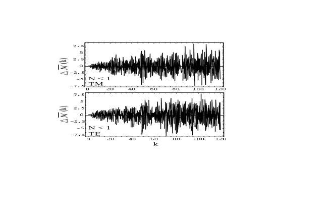
Figure 1: The fluctuating part of the spectral counting function for the TM and TE theories ($r/R=2/10$ and $N=3/4$).

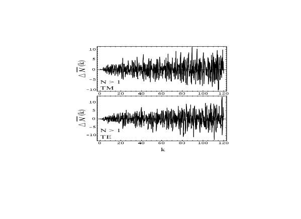
Figure 2: The fluctuating part of the spectral counting function for the TM and TE theories ($r/R=2/10$ and $N=3$).

VI Conclusion and perspectives

a) From our previous results obtained in the particular case of annular ray-splitting billiards, we can infer rules permitting us to construct Weyl formulas for general ray-splitting billiards. The associated Weyl formulas providing the smoothed spectral counting functions are given in the usual form, i.e., by

$$\bar{\mathcal{N}}(k)\approx\frac{\mathcal{A}}{4\pi}k^{2}+\frac{\mathcal{L}}{4\pi}k+\mathcal{C},$$ (41)

but now, the area term $\mathcal{A}$, the perimeter term $\mathcal{L}$ as well as the constant term $\mathcal{C}$ must take into account the ray-splitting phenomenon:

(i) $\mathcal{A}$ is the billiard total area weighted by the refraction index. For example, a piece of billiard of area $a$ and index of refraction $N$ provides a contribution to $\mathcal{A}$ given by

$$N^{2}a.$$ (42)

(ii) $\mathcal{L}$ is a sum of terms associated with the boundaries on which discontinuities in the physical properties occur. The contribution of a boundary of length $\ell$ which separates a region of index $N$ from a forbidden region is given by

$$-N\ell$$ (43)

if we assume Dirichlet condition on that boundary and by

$$N\ell$$ (44)

if we assume Neumann condition. The contribution of a boundary of length $\ell$ which separates a region of index $N$ from a region of index $1$ is given by

$$\left[\frac{4}{\pi}\,E(1-N^{2})-N-1\right]\ell\quad\mathrm{if}\quad N<1,$$ (45a)

$$\left[\frac{4N}{\pi}\,E\left(\frac{N^{2}-1}{N^{2}}\right)-N-1\right]\ell\quad\mathrm{if}\quad N>1,$$ (45b)

for the TM polarization, by

$$\left[\frac{4}{\pi}\,\frac{N^{2}}{1+N^{2}}\,K(1-N^{2})+\frac{4}{\pi}\,\frac{N^{4}}{1+N^{2}}\,\Pi\left(1-N^{4},\frac{\pi}{2},1-N^{2}\right)-N-1\right]\ell\quad\mathrm{if}\quad N<1,$$ (46a)

$$\left[\frac{4}{\pi}\,\frac{N}{1+N^{2}}\,K\left(\frac{N^{2}-1}{N^{2}}\right)+\frac{4}{\pi}\,\frac{1}{N(1+N^{2})}\,\Pi\left(\frac{N^{4}-1}{N^{4}},\frac{\pi}{2},\frac{N^{2}-1}{N^{2}}\right)-N-1\right]\ell\quad\mathrm{if}\quad N>1,$$ (46b)

for the TE polarization and by

$$\left[\frac{4}{\pi}\,\frac{\alpha(1-N^{2})}{\alpha^{2}-1}\,K(1-N^{2})+\frac{4}{\pi}\,\frac{\alpha^{2}N^{2}-1}{\alpha(\alpha^{2}-1)}\,\Pi\left(\frac{\alpha^{2}-1}{\alpha^{2}},\frac{\pi}{2},1-N^{2}\right)-N-1\right]\ell\quad\mathrm{if}\quad N<1,$$ (47a)

$$\left[\frac{4}{\pi}\,\frac{\alpha(1-N^{2})}{N(\alpha^{2}-1)}\,K\left(\frac{N^{2}-1}{N^{2}}\right)+\frac{4}{\pi}\,\frac{\alpha(\alpha^{2}N^{2}-1)}{N(\alpha^{2}-1)}\,\Pi\left(1-\alpha^{2},\frac{\pi}{2},\frac{N^{2}-1}{N^{2}}\right)-N-1\right]\ell\quad\mathrm{if}\quad N>1,$$ (47b)

in the general case ($\alpha\not=1$).

(iii) The constant term $\mathcal{C}$ takes into account curvature and corner contributions. As far as the former is concerned, it is given by

$$+\frac{1}{12\pi}\int_{\Gamma}\frac{ds}{R(s)}$$ (48)

for a boundary curve $\Gamma$ which separates a region of index $N$ from a forbidden region, $R(s)$ denoting the local radius of curvature along $\Gamma$. When $\Gamma$ is a ray-splitting boundary which separates a region of index $N$ from a region of index $1$ the associated curvature contribution vanishes. As far as corner contributions are concerned, we simply note that ray-splitting corners with angle $\pi/2$ provide a vanishing contribution.

We are just beginning to check the previous formulas for the various desymmetrized versions of ray-splitting sinai billiards. We obtain a very good agreement between the theoretical formulas and the numerical data. This reinforces our opinion that they are exact. It would be very interesting to prove them rigorously but we are unable to do so. We have also tried to link the formulas found for the TM polarization ($\alpha=1$) to the results that Kohler and Blümel Kohler and Blümel (1998c) have obtained for the scaled states of quantum ray-splitting billiards. We believe that such a link must exist but, unfortunately, we have not established it.

b) In this paper, we have been exclusively concerned with the smooth part of the spectral counting function ${\cal N}(k)$ for annular ray-splitting billiards. It seems to us possible to treat also the construction of the oscillating part of ${\cal N}(k)$ as a canonical problem. By carefully taking into account Stokes phenomenon in the context of hyperasymptotics Berry (1989); Berry and Howls (1991), it might be possible to extract from $g(s)$ all the periodic orbit contributions, even though the algebraic calculations involved are certainly enormous.

c) Finally, it would be very interesting to extend our calculations to the three-dimensional case, having in mind applications to the domain of quantum optics and more particularly to cavity quantum electrodynamics. Indeed, as it is well-known, the optical properties (spontaneous emission, stimulated emission, … ) of atoms and molecules embedded in a cavity strongly depend on the density of states of the electromagnetic field. Because of that, Weyl formulas for cavities containing dielectric structures would be certainly welcome.

References

• Weyl (1911) H. Weyl, Nachr. Akad. Wiss. Gø̈ttingen p. 110 (1911).
• Kac (1966) M. Kac, Am. Math. Monthly 73, 1 (1966).
• Baltes and Hilf (1976) H. T. Baltes and E. R. Hilf, Spectra of Finite Systems (Bibliographisches Inst. Wissenschaftsverlag, Mannheim, 1976).
• Brack and Bhaduri (1997) M. Brack and R. K. Bhaduri, Semiclassical Physics (Addison-Wesley, Reading, 1997).
• Balian and Bloch (1970) R. Balian and C. Bloch, Ann. Phys. (N.Y.) 60, 401 (1970).
• Balian and Bloch (1971) R. Balian and C. Bloch, Ann. Phys. (N.Y.) 64, 271 (1971).
• Stewartson and Waechter (1971) K. Stewartson and R. T. Waechter, Proc. Camb. Phil. Soc. 69, 581 (1971).
• Berry and Howls (1994) M. Berry and C. J. Howls, Proc. R. Soc. Lond. A 447, 527 (1994).
• Sieber et al. (1995) M. Sieber, H. Primack, U. Smilansky, I. Ussishkin, and H. Schanz, J. Phys. A: Math. Gen. 28, 5041 (1995).
• Couchman et al. (1992) L. Couchman, E. Ott, and T. M. Antonsen, Phys. Rev. A 46, 6193 (1992).
• Prange et al. (1996) R. E. Prange, E. Ott, T. M. Antonsen, B. Georgeot, and R. Blümel, Phys. Rev. E 53, 207 (1996).
• Blümel et al. (1996a) R. Blümel, T. M. Antonsen, B. Georgeot, E. Ott, and R. E. Prange, Phys. Rev. Lett. 76, 2476 (1996a).
• Blümel et al. (1996b) R. Blümel, T. M. Antonsen, B. Georgeot, E. Ott, and R. E. Prange, Phys. Rev. E 53, 3284 (1996b).
• Kohler and Blümel (1998a) A. Kohler and R. Blümel, Phys. Lett. A 238, 271 (1998a).
• Kohler and Blümel (1998b) A. Kohler and R. Blümel, Phys. Lett. A 247, 87 (1998b).
• Kohler and Blümel (1998c) A. Kohler and R. Blümel, Ann. Phys. (N.Y.) 267, 249 (1998c).
• Dabaghian et al. (2001) Y. Dabaghian, R. V. Jensen, and R. Blümel, Phys. Rev. E 63, 066201 (2001).
• Savytskyy et al. (2001) N. Savytskyy, A. Kohler, S. Bauch, R. Blümel, and L. Sirko, Phys. Rev. E 64, 036211 (2001).
• Blümel et al. (2002) R. Blümel, Y. Dabaghian, and R. V. Jensen, Phys. Rev. E 65, 046222 (2002).
• Jones (1986) D. S. Jones, Acoustic and Electromagnetic Waves (Clarendon Press, Oxford, 1986).
• Wolfram (1996) S. Wolfram, The Mathematica book (Cambridge University Press, Cambridge, 1996).
• Abramowitz and Stegun (1965) M. Abramowitz and I. A. Stegun, Handbook of Mathematical Functions (Dover, New-York, 1965).
• Howls and Trasler (1998) C. J. Howls and S. A. Trasler, J. Phys. A: Math. Gen. 31, 1911 (1998).
• Howls and Trasler (1999) C. J. Howls and S. A. Trasler, J. Phys. A: Math. Gen. 32, 1487 (1999).
• Berry (1989) M. Berry, Proc. R. Soc. Lond. A 422, 7 (1989).
• Berry and Howls (1991) M. Berry and C. J. Howls, Proc. R. Soc. Lond. A 434, 657 (1991).
• Gradshteyn and Ryzhik (1994) I. S. Gradshteyn and I. M. Ryzhik, Table of Integrals, Series, and Products (Academic Press, San Diego, 1994), 5th ed.