(Vanishing) Twist in the Saddle-Centre and Period-Doubling Bifurcation

Abstract

The lowest order resonant bifurcations of a periodic orbit of a Hamiltonian system with two degrees of freedom have frequency ratio $1:1$ (saddle-centre) and $1:2$ (period-doubling). The twist, which is the derivative of the rotation number with respect to the action, is studied near these bifurcations. When the twist vanishes the nondegeneracy condition of the (isoenergetic) KAM theorem is not satisfied, with interesting consequences for the dynamics. We show that near the saddle-centre bifurcation the twist always vanishes. At this bifurcation a “twistless” torus is created, when the resonance is passed. The twistless torus replaces the colliding periodic orbits in phase space. We explicitly derive the position of the twistless torus depending on the resonance parameter, and show that the shape of this curve is universal. For the period doubling bifurcation the situation is different. Here we show that the twist does not vanish in a neighborhood of the bifurcation.

Keywords: Twist Maps; Hamiltonian Systems; Saddle-Centre Bifurcation; Period-doubling Bifurcation; KAM; Normal Forms; Elliptic Integrals

1 Introduction

The dynamics near a periodic orbit of a Hamiltonian system can be studied in terms of a local Poincaré section transversal to the orbit. In two degrees of freedom the first return map restricted to the surface of constant energy is an area preserving map with a fixed (or periodic) point. If the multipliers $\mu_{i}$, $i=1,2$ of the fixed point have modulus 1 (but are not equal to $\pm 1$) the fixed point is called elliptic. Then $\mu_{1}=\overline{\mu_{2}}\in\mathbb{C}$ and we can write $\mu=\exp(2\pi i\omega)$ with the rotation number $0<\omega<1/2$ of the periodic orbit. If the periodic orbit is elliptic and the rotation number is irrational the map can (formally) be transformed to Birkhoff normal form which in action-angle variables $(\varphi,I)$ reads

$$(\varphi,I)\to(\varphi+2\pi\Omega(I),I)\,.$$ (1)

The action $I$ is like the radial coordinate in polar coordinates, hence the map in normal form maps circles to circles by rotating them $\Omega(I)$ times. The rotation number (or winding number) $\Omega(I)$ near the periodic orbit can be expanded as

$$\Omega(I)=\omega+\tau_{0}I+\frac{1}{2}\tau_{1}I^{2}+...$$

The twist (or torsion) $\tau(I)$ is the derivative of the rotation number with respect to the action,

$$\tau(I)=\frac{{\rm d}\Omega}{{\rm d}I}(I)=\tau_{0}+\tau_{1}I+...$$

When the rotation number is a strictly monotone function of the action in some interval the map (1) restricted to the corresponding annulus is called a monotone twist map. Moser’s KAM theorem [11] states that the invariant torus $I=I_{0}$ of (1) persist under perturbation when its frequency $\Omega(I_{0})$ is diophantine and its twist $\tau(I_{0})$ does not vanish. Arnold’s KAM theorem [1] is the same statement for flows where the nonvanishing of the twist corresponds to the isoeneregetic nondegeneracy conditions. A well known corollary of the KAM theorem is the stability of an elliptic fixed point in two degrees of freedom when $\Omega(0)=\omega\not=1/3,1/4$ and the twist at the origin is non-vanishing, $\tau(0)=\tau_{0}\not=0$.

When the twist vanishes the perturbed dynamics can be more complicated. The stability of an elliptic point can be lost when its twist vanishes, see [5] for an example of an unstable elliptic point with $\omega=1/5$. The effects of vanishing twist away from the origin was first described by Howard [7], and the resulting effects have been observed in many examples [13, 10]. The probably most spectacular effect is the appearance of so-called meandering curves [7, 6, 12]. The properties of non-twist maps also show interesting behaviour under renormalisation [2] and recently it has been shown [3] that an extension of the KAM theorem can also be proved in this context. In [5, 9] it was finally shown that the vanishing of twist at the fixed point generically occurs in a one parameter family when the rotation number of a fixed point passes through the interval $[1/4,1/3]$. When the twist vanishes at the fixed point a twistless torus is created in a twistless bifurcation [5]. After creation the twistless torus passes through resonances and in this way non-twist maps generically appear in one parameter families of area preserving maps. The truncated resonant Birkhoff normal form shows that this twistless torus eventually collides with a saddle-centre bifurcation that gives rise to the period 3 orbits that collide with the fixed point when $\omega=1/3$ [5]. Such a connection between resonance and vanishing twist can also be found in 4 dimensional symplectic maps [4].

The techniques of [5] can also be applied to the higher order resonances, in particular for $\omega=1/4$. In this paper we study the two remaining generic bifurcations at even stronger resonance $\omega=0,1/2$. By definition the corresponding fixed point is not elliptic. The two cases will be denoted as the $1:1$ and $1:2$ resonance, or as the saddle-centre and period doubling bifurcation, respectively. The main result is that near the saddle-centre bifurcation the twist always vanishes, while it does not vanish near the period doubling bifurcation.

The method is based on the analysis of the resonant normal form, in which the Poincaré map is approximated by the time $1$ map of a one degree of freedom system, see e.g. [8]. This normal form is an approximation, that is local near the bifurcation in parameter space and in phase space. At first we will completely ignore this, and just analyse the normal forms in the following two sections. In section 4 we will address the problem of non-locality in phase space, and also comment on the effect of higher order perturbations on the twistless tori. We will talk of invariant tori even though the invariant curves $H(u,v)=h$ of the normal form may not be compact. This will also be justified in Sec. 4. Finally we treat a saddle-centre bifurcation in the Hénon map as an example.

2 Saddle-Centre Bifurcation

The normal form of a Hamiltonian system with two degrees of freedom near the $1:1$ resonance has the form

$$H(u,v)=\frac{v^{2}}{2}+\frac{u^{3}}{3}+\varepsilon u\,.$$ (2)

The coefficient of $u^{3}$ has been scaled so that it equals $1/3$. The variables $u$ and $v$ are canonically conjugate variables on a local transversal Poincaré section and $\varepsilon$ is a parameter, typically the energy of the original system. The Poincaré map is given by the time $1$ map of the flow of $H(u,v)$. If the period $T$ is large, the time $1$ map advances little. The rotation number of the full system is the period $1$ divided by the period of the reduced one degree of freedom flow, $\Omega=1/T$. The more familiar $\Omega=2\pi/T$ is obtained when the time $2\pi$ map is taken instead of the time $1$ map, but the time $1$ map is more natural at least for the example of the Hénon map we are going to discuss. Since $\Omega$ is determined by $T$, we now study in detail the period $T$ of the one degree of freedom system given by $H$.

The critical points and critical values of the energy map $H:\mathbb{R}^{2}\to\mathbb{R}$ and their dependence on $\varepsilon$ give the main structure to the bifurcation. Instead of a one degree of freedom system $H(u,v;\varepsilon)$ depending on the parameter $\varepsilon$ one may consider $H(u,v,\varepsilon,\theta)$ as a Hamiltonian in $\mathbb{R}^{3}\times S^{1}$, with action $\varepsilon$ and conjugate angle $\theta$. The set of critical values of the energy-momentum map $(H,\varepsilon):\mathbb{R}^{3}\times S^{1}\to\mathbb{R}^{2}$ is called the bifurcation diagram. A simple way to compute it is to find the critical values of the energy map of $H(u,v)$ and consider their parameter dependence on $\varepsilon$. The Hamiltonian has critical points $(u,v)=(\pm\sqrt{-\varepsilon},0)$ and corresponding critical values $h=\mp 2(-\varepsilon)^{3/2}/3$. They exist when $\varepsilon<0$ and the upper sign corresponds to a local minimum of $H$, while the lower sign gives a saddle. The corresponding phase portraits are shown in Fig. 1.

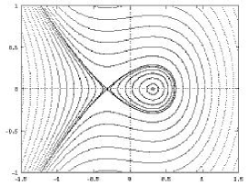
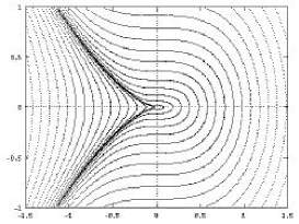
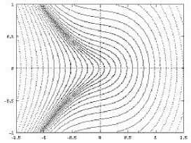
Figure 1: Lines of constant energy on the phase space $(u,v)$ for the saddle-centre bifurcation ($1:1$ resonance, $\omega=0$). left: $\varepsilon=-0.1$, middle: $\varepsilon=0$, right: $\varepsilon=0.1$.

The dynamics is given by Hamiltons equation $\dot{u}=v$ and eliminating $v$ using the Hamiltonian gives a first order equation for $u$. After separation of variables the period of motion with energy $h$ is given by the elliptic integral

$$T(h,\varepsilon)=\oint\frac{{\rm d}u}{\sqrt{2h-\frac{2}{3}u^{3}-2\varepsilon u}}\,,$$ (3)

where the integration path is encircling the interval on the real axis where the argument of the square root is positive. If there are two positive intervals either one can be taken, the result is the same. By scaling $u=z(\sigma\varepsilon)^{1/2}$, where $\sigma={\rm sign}(\varepsilon)$ and introducing the one essential parameter

$$\gamma=\frac{3h}{2(\sigma\varepsilon)^{3/2}}\,,$$ (4)

the period $T$ is an elliptic integral on the curve

$${\cal E}:w^{2}=P_{3}(z)=2\gamma-z^{3}-3\sigma z\,.$$ (5)

The case $\varepsilon=0$ has to be excluded in this scaling, but it is simple to treat it separately. We are mostly interested in the case where $\sigma=1$. The essential integral now reads

$$S(\gamma)=\oint\frac{1}{w}\,{\rm d}z$$ (6)

and it is related to the period by

$$T(h,\varepsilon)=\frac{\sqrt{3/2}}{(\sigma\varepsilon)^{1/4}}S(\gamma)\,.$$ (7)

The polynomial $P_{3}$ has one or three real roots. The collision of two real roots corresponds to the unstable equilibrium and its separatrix. It occurs when the discriminant

$$\Delta=-108(\sigma+\gamma^{2})$$

vanishes. $\Delta=0$ is only possible for $\sigma=-1$ and hence the critical parameters for which a double root occurs are given by $\gamma=\pm 1$, hence

$$9h^{2}=-4\varepsilon^{3}\,,$$ (8)

which has a cusp at the origin. At the origin $h=\varepsilon=0$ all three roots collide in the saddle-centre bifurcation. The discriminant (8) is shown in Fig. 2.

Figure 2: Schematic sketch of the bifurcation diagram for the saddle-centre bifurcation. Graphs of $P_{3}$ are shown together with a horizontal line indicating the value of $h$. The bold lines are the critical values of the saddle.

In the case of the saddle-centre bifurcation the bifurcation diagram is given by the discriminant of $P_{3}$. The bifurcation diagram divides the parameter plane $(\varepsilon,h)$ into two regions: one with 3 real roots and one with 1 real and two complex roots. The latter has positive $\varepsilon$ everywhere, while the former is the wedge shaped region contained in the negative half-plane. For $\varepsilon<0$ the phase portraits contain a pair of stable/unstable fixed points. The critical value of the energy of the stable fixed point is a local minimum given by the lower branch of the bifurcation diagram, while that of the unstable fixed point is a saddle given by the branch with positive $h$. For this range of energies there are 3 real roots. It will turn out that the upper branch of the bifurcation diagram corresponding to the unstable fixed point is crucial for the existence of vanishing twist. For $\varepsilon>0$ the phase portrait is without fixed points. Even though the topology is trivial in this case we will now show that the rotation number has a maximum on a certain invariant torus containing points near the origin in the phase space. At this maximum of the rotation number the twist vanishes. The vanishing twist occurs at the vertical tangents of the contours of the rotation number shown in Fig. 3. The fact that the invariant curves are all unbounded for $\varepsilon>0$ will be dealt with in section 4. For now observe that the integral (3) is finite, even though the invariant curves are unbounded in $v$.

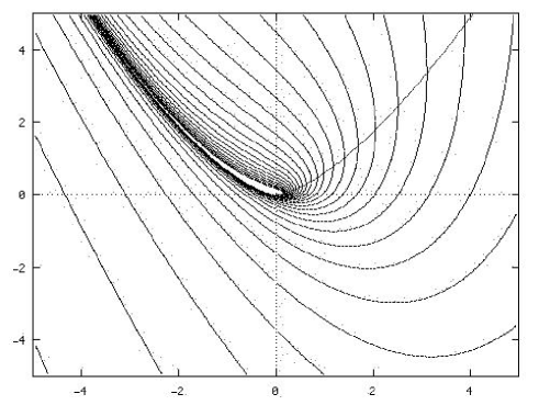
Figure 3: Lines of constant period $T=1/\Omega$ equidistant with $\Delta T=0.3$ on the parameter plane $(\varepsilon,h)$ for the saddle-centre bifurcation ($1:1$ resonance, $\omega=0$). The vanishing twist is indicated by a curve of vertical tangents $\partial\Omega/\partial h=0$.

The main feature of the level lines of the rotation number as shown in Fig. 3 is that it diverges when the unstable periodic orbit is approached. This occurs for the positive critical value of $h$ when $\varepsilon<0$. Everywhere else the rotation number is a well defined, smooth and bounded function of $h$ and $\varepsilon$. Accordingly the level lines “hug” the curve of critical values that correspond to the unstable orbit. Already from this property one can deduce the existence of a curve with vanishing twist using topological arguments. Here we proceed along the analytical route, because it will give us more detailed information. Note that the curve of critical values with negative $h$, see Fig. 2, does not appear in Fig. 3. One reason for this is that we chose to plot the rotation number for the (non-compact) invariant tori with motion between $-\infty$ and the smallest real zero of $P_{3}$. These invariant tori do not contain critical points of the energy map, even though the corresponding energy might be a critical value. Accordingly the rotation number is smooth across this line of critical values. The critical point corresponding to the critical values is the stable fixed point at the local minimum of $H$. But even if we would plot the rotation number of the bounded invariant tori near the local minimum of the potential the picture is unchanged. The reason is that for a cubic elliptic curve the integrals of first kind over either one of the two real intervals (if they exist) are equal.

Since $\Omega=1/T$ and $2\pi T=\partial J/\partial h$ the derivative of the rotation function is

$$\frac{\partial\Omega}{\partial J}=\frac{\partial\Omega/\partial h}{\partial J/\partial h}=-\frac{\partial T/\partial h}{2\pi T^{3}}\,.$$

Hence the twist vanishes when

$$\frac{\partial T}{\partial h}=\frac{(3/2)^{3/2}}{\varepsilon^{7/4}}\frac{\partial S}{\partial\gamma}=0$$

and this is only possible for finite $\varepsilon$ when

$$\frac{\partial S}{\partial\gamma}=-\oint\frac{1}{w^{3}}\,{\rm d}z=0\,.$$

This complete elliptic integral can be written as a linear combination of Legendre’s standard integrals. In this way a condition for the vanishing of the twist is now obtained. The relevant case for this purpose is that of one real root, for which the phase portrait has no fixed point. The integrand $w$ is positive for $u\in(-\infty,z_{0})$, where $z_{0}$ is the single root of $P_{3}(z)$. Let the factorized polynomial be given by

$$P_{3}(z)=-(z-z_{0})P_{2}(z),\qquad P_{2}(z)=(z-\zeta_{1})^{2}+\zeta_{2}^{2}\,,$$ (9)

so that the complex roots are $\zeta_{1}\pm i\zeta_{2}$. Denote the distance between the real and complex roots by $r$, hence $r^{2}=P_{2}(z_{0})$, so that the discriminant is given by $\Delta=-4r^{4}\zeta_{2}^{2}$. Legendre’s standard integral of the first kind $K(k)$ has differential

$$\omega_{1}=\frac{1}{\sqrt{P_{3}(z)}}{\rm d}z$$ (10)

up to a constant factor, where the modulus $k$ is given by

$$k^{2}=\frac{1}{2}\left(1+\frac{z_{0}-\zeta_{1}}{r}\right)=\frac{1}{2}\left(1+\frac{{\rm sign}(\gamma)}{\sqrt{1+\alpha^{2}}}\right)\,,$$ (11)

and in the last equality the parameter $\alpha=\zeta_{2}/(z_{0}-\zeta_{1})$ has been introduced. In the second equality in addition ${\rm sign}(z_{0}-\zeta_{1})={\rm sign}(\gamma)$ is used, which is true because $z_{0}=\zeta_{1}$ in (9) together with the vanishing of the quadratic coeffcient in (5) implies $z_{0}=\zeta_{1}=0$, and therefoe the polynomial has no constant term and $h=\gamma=0$.

A non-standard form of the differential of Legendre’s standard integral of second kind $E(k)$ is

$$\omega_{2}=\frac{P_{2}(z){\rm d}z}{(z-(z_{0}\pm r))^{2}}\omega_{1}\,,$$

up to the same constant factor as in (10). The differential ${\mathrm{d}}z/w^{3}$ we are interested in is of the second kind, and can therefore be written as a linear combination of $\omega_{1}$ and $\omega_{2}$ with constant coefficients, up to a total differential:

$$\frac{{\rm d}z}{w^{3}}=A\omega_{1}+B\omega_{2}+{\rm d}F$$

where $F=Q_{2}(z)/((z-(z_{0}\pm r))w)$. Together with the undetermined coefficients of the quadratic polynomial $Q_{2}$ this gives a system of 5 linear equations for the 5 unknown coefficients. Solving these equations gives

$$A=\frac{2r}{\Delta}((z_{0}-\zeta_{1})r-r^{2}+4\zeta_{2}^{2}),\quad B=\frac{4r}{\Delta}(r^{2}-4\zeta_{2}^{2})$$

Since the quadratic coefficient of $P_{3}$ is zero, the roots of $P_{3}$ add up to zero. Therefore the real parts satisfy $z_{0}+2\zeta_{1}=0$, hence

$$2k^{2}=1-3\zeta_{1}/r\quad\mbox{and}\quad r^{2}=9\zeta_{1}^{2}+\zeta_{2}^{2}\,.$$

With these equations the coefficients $A$ and $B$ can be expressed in terms of $k$ alone, up to the factor $(r^{2}\Delta)^{-1}$. The condition of vanishing twist, $\partial S/\partial\gamma=0$, finally reads

$$(8k^{4}-9k^{2}+1)K(k)=(16k^{4}-16k^{2}+1)E(k)\,,$$

where $K(k)$ and $E(k)$ stand for elliptic integrals of the first and the second kind, respectively.

For $k=0$ we have equality since both elliptic integrals equal $\pi/2$. The first derivatives of either side vanishes, but the second derivatives are $-35\pi/4$ and $-65\pi/4$, respectively, so that the left hand side is larger for small $k$. For $k=1$ the prefactor of $K$ vanishes, while that of $E$ gives 1 and $E(1)=1$. Hence for $k\to 1$ the right hand side dominates. This proves that there exists a solution of this equation for $k\in(0,1)$. Numerically we find $k_{0}^{2}\approx 0.7097215$. In order to calculate the corresponding $\gamma_{0}$ we observe that $\alpha$ as introduced in (11) is related to $\gamma$ by

$$\alpha=\frac{\zeta_{2}}{z_{0}-\zeta_{1}}=-\frac{\zeta_{2}}{3\zeta_{1}}=\frac{1}{\sqrt{3}}\frac{\Gamma^{2}+\sigma}{\Gamma^{2}-\sigma}\,,$$ (12)

where

$$\Gamma=(\gamma+\sqrt{\sigma+\gamma^{2}})^{1/3}\,.$$ (13)

Using (11) and $k_{0}$ the corresponding value of $\alpha$ is $\alpha_{0}\approx 2.164255$, and from $\alpha_{0}$ using (12) we find $\gamma_{0}\approx 0.9152203$. Therefore the curve of vanishing twist in the parameter plane occurs for positive $\varepsilon$ when

$$3h=2\gamma_{0}\varepsilon^{3/2}\,.$$ (14)

Since $\gamma_{0}<1$ the curve of vanishing twist is bent downward as compared to the bifurcation curve (8) for $\varepsilon<0$ and $h>0$. See Fig. 3 for a graph of this curve together with the numerically computed lines of constant rotation number. The lines of constant rotation number have vertical slope at their intersection with the critical curve, as must be the case.

Figure 4: Bifurcation diagram of the position in phase space $u$ versus the bifurcation parameter $\varepsilon$. For $\varepsilon<0$ the location of the fixed points at $\pm\sqrt{-\varepsilon}$ are shown, while for $\varepsilon>0$ the maximal $u$ of the twistless torus at $z_{0}(\gamma_{0})\sqrt{\varepsilon}$ is shown.

The scaling of $u$ reduces the number of parameters to one. The essential parameter $\gamma$, in its dependence on $h$ and $\varepsilon$, organizes the bifurcation. It allows to compute explicitly all the important characteristics of the twistless torus. Combining (11) and (12) shows that $k$ is a function of $\gamma$. The curves in the parameter plane that have the same value of $\gamma$ are given by (4). The most prominent ones are the curve of critical values $\gamma=\pm 1$, as shown in Fig. 2, and $\gamma=\gamma_{0}$, the curve of twistless tori, see Fig. 3. They all have the same shape of a semicubical parabola, except when $\gamma=0$, hence $h=0$, or $\gamma=\pm\infty$, hence $\varepsilon=0$ with $\pm h>0$.

$$\begin{array}[]{cccc}k^{2}&\gamma&\alpha&\text{curve}\\ \hline\cr 1&+1&0&3h=-2(-\varepsilon)^{3/2}\\ \frac{1}{4}(2+\sqrt{3})&+\infty&{1}/{\sqrt{3}}&\varepsilon=0,h>0\\ 0.709721497&0.91522&2.164255&3h=\gamma_{0}(-\varepsilon)^{3/2}\\ \frac{1}{2}&0&\infty&\varepsilon=0,h>0\\ \frac{1}{4}(2-\sqrt{3})&-\infty&{1}/{\sqrt{3}}&\varepsilon=0,h<0\\ 0&-1&0&3h=2(-\varepsilon)^{3/2}\end{array}$$

Approaching the bifurcation point along the curve (4) gives $k(\gamma)$ in the limit. The function $k(h,\varepsilon)$ is therefore not continuous at the origin. Moving on curves (4) in the parameter plane for any $\gamma\neq 1$ the change in the period $T(h,\varepsilon)$ given by (3) is elementary. From (7) it follows that $T$ is proportional to $|\varepsilon|^{-1/4}$, and the constant of proportionality is determined from (7) and (6). The divergence of the period upon approaching the bifurcation is therefore not caused by the elliptic integral, but merely by the algebraic dependence $|\varepsilon|^{-1/4}$. In this way the rotation number of the stable periodic orbit is given by

$$\Omega(\gamma=-1,\varepsilon)=\frac{1}{\sqrt{2}\pi}(-\varepsilon)^{1/4}\approx 0.225079\,|\varepsilon|^{1/4}\,.$$

The integral $S(-1)$ contained in this expression can be easily calculated using residue calculus because for $\gamma=-1$ the curve has a double root, $P_{3}(z)=-(z+2)(z-1)^{2}$. For general values of $\gamma$ and in particular for the twistless torus the elliptic integral $S(\gamma)$ (6) needs to be calculated. The single real root is given by

$$z_{0}=\Gamma-\frac{\sigma}{\Gamma},\quad\text{hence}\quad z_{0}(\gamma_{0})\approx 0.5535942\,.$$ (15)

Finally $S(\gamma)$ is obtained as

$$S(\gamma)=\frac{4K(k)}{\sqrt{3z_{0}\sqrt{1+\alpha^{2}}/2}}\,.$$

In particular when $\gamma=\gamma_{0}$ the rotation number of the twistless torus is

$$\Omega(\gamma=\gamma_{0},\varepsilon)=\frac{\sqrt{z_{0}(\gamma_{0})\sqrt{1+\alpha^{2}_{0}}}}{4K(k_{0})}\varepsilon^{1/4}\approx 0.1374244\,\varepsilon^{1/4}\,.$$ (16)

The constant of proportionality is close to $\sqrt{3}/4\pi$. Using the above value of $z_{0}$ the position of the rightmost point of the twistless torus in phase space is located at $u_{0}=z_{0}\sqrt{\varepsilon}$. This means that for $\varepsilon=\varepsilon_{0}$ this point is on the same side as the stable periodic orbit was for $\varepsilon=-\varepsilon_{0}$ before the bifurcation, but by a factor of $1/z_{0}(\gamma_{0})\approx 2$ closer to the origin. See Fig. 4 for an illustration in the form of a standard bifurcation diagram showing position in phase space $u$ versus bifurcation parameter $\varepsilon$.

3 Period-Doubling Bifurcation

The normal form of a Hamiltonian system with two degrees of freedom near a periodic orbit in $1:2$ resonance is

$$H(u,v)=\frac{v^{2}}{2}+D\frac{u^{4}}{4}+\varepsilon u^{2}\,,$$ (17)

where $D=\pm 1$. As in the case of the saddle-centre bifurcation the variables $u$ and $v$ are canonically conjugate variables on a local transversal Poincaré section and $\varepsilon$ is a parameter, typically corresponding to the energy of the original system. Contourplots of this Hamiltonian show the intersection of invariant tori with the Poincaré section transversal to the bifurcating orbit. For $D=1$ they are shown in Fig. 5, for $D=-1$ in Fig. 6, for $\varepsilon<0$, $\varepsilon=0$, and $\varepsilon>0$, respectively.

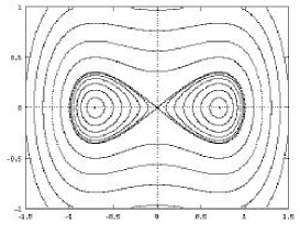
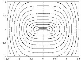
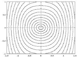
Figure 5: Lines of the constant energy on the phase space $(u,v)$ for the period-doubling bifurcation $(D=1)$ for $\varepsilon=-0.1$, $\varepsilon=0$, $\varepsilon=0.1$.

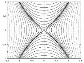
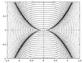
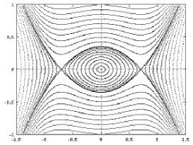
Figure 6: Lines of the constant energy on the phase space $(u,v)$ for the period-doubling bifurcation $(D=-1)$, for $\varepsilon=-0.1$, $\varepsilon=0$, $\varepsilon=0.1$

The critical points and critical values of the energy map $H:\mathbb{R}^{2}\to\mathbb{R}$ and their dependence on the parameter $\varepsilon$ describe the structure of the bifurcation. The Hamiltonian has critical points at $(0,0)$ and at $(u,v)=(\pm\sqrt{-2\varepsilon D},0)$ with critical values $h=0$ and $h=-D\varepsilon^{2}$. The origin is a local minimum for $\varepsilon>0$, a saddle otherwise. The second critical point exists when $\varepsilon D<0$, and is a local minimum for $\varepsilon<0$, a saddle otherwise. The set of critical values, see Fig. 7, therefore is the union of the line $h=0$ with the half of the parabola $h=-D\varepsilon^{2}$ for which $D\varepsilon<0$. For $D>0$ the only unstable branch in the bifurcation diagram is $h=0$ for $\varepsilon<0$. It divides the two regions of real motion. A third region $\{h<-\varepsilon^{2}\}\cup\{\varepsilon>0,-\varepsilon^{2}<h<0\}$ is not in the image of $H$, hence there is no real motion corresponding to $(h,\varepsilon)$ from this region.

For $D<0$ the line of critical values $h=0$ again has a saddle as critical point when $\varepsilon<0$. In addition the half parabola $h=\varepsilon^{2}$, $\varepsilon>0$ also corresponds to a saddle of $H$ that is not at the origin. When $D<0$ the whole plane $(h,\varepsilon)$ is in the image of $H$ considering all $\varepsilon$. The critical values divide the plane into three regions with 0, 2, and 4 real roots.

Figure 7: Schematic sketch of the bifurcation diagram for the two cases of the period doubling bifurcation. Graphs of $P_{4}$ are shown together with a horizontal line indicating the value of $h$. The bold line denote critical values of unstable orbits. The dashed line is not critical; it indicates a vanishing of the discrimiant.

The dynamics of the reduced one degree of freedom system is given by $\dot{u}=v$ and eliminating $v$ using the Hamiltonian gives a first order equation for $u$. Separation of variables then gives the period of motion in the reduced one degree of freedom system as the elliptic integral

$$T(h,\varepsilon)=\oint\frac{{\rm d}u}{\sqrt{2h-\frac{1}{2}Du^{4}-2\varepsilon u^{2}}}\,.$$

The number of parameters could be reduced by introducing the ratio $h/\varepsilon^{2}$, but for clarity we do not introduce this scaling. The period $T$ is an elliptic integral on the curve

$${\cal E}:w^{2}=P_{4}(z)=P_{2}(z^{2})=2h-\frac{1}{2}Dz^{4}-2\varepsilon z^{2}\,.$$ (18)

The discriminant of $P_{4}$ is

$$\Delta=-256Dh(Dh+\varepsilon^{2})^{2}\,.$$

It vanishes for $h=0$ and $Dh=-\varepsilon^{2}$, corresponding to the critical values $h=0$ and $h=-D\varepsilon^{2}$ already found above. As usual the set of critical values is contained in the discriminant, however, the discriminant vanishes on a larger set. Namely the branch of the parabola with $D\varepsilon>0$ is not part of the critical values. The three regions already found correspond to regions with 4, 2, and 0 real roots of $P_{4}$, respectively, see Fig. 7. The part of the discriminant that is not part of the critical values is dashed. The polynomial can be factored as

$$P_{4}(z)=-\frac{1}{2}D(\xi_{-}-z^{2})(\xi_{+}-z^{2}),\quad\frac{1}{2}D\xi_{\pm}=-\varepsilon\pm\sqrt{\varepsilon^{2}+Dh}\,.$$

Comparing coefficients gives $\xi_{-}\xi_{+}=-4hD$ and $\xi_{-}+\xi_{+}=-4\varepsilon D$. The factorization of $P_{4}$ has real factors, i.e. $\xi_{\pm}\in\mathbb{R}$, with one exception. It occurs when the quadratic equation $P_{2}(\xi)=0$ has complex roots. The position of the roots in the regions of the parameter plane is as follows. The two real cases for $D=1$ are

$$+2: h>0 \xi_{-}<0<\xi_{+} 2[-\sqrt{\xi_{+}},\sqrt{\xi_{+}}]$$

$$+4: \varepsilon<0,-\varepsilon^{2}<h<0 0<\xi_{-}<\xi_{+} 2[\sqrt{\xi_{-}},\sqrt{\xi_{+}}]$$

In the first column a label is given containing the number of real roots. All 4 cases appear when $D=-1$ for

$$-2: h<0 \xi_{+}<0<\xi_{-} 2[-\infty,-\sqrt{\xi_{-}}]$$

$$-4: \varepsilon>0,0<h<\varepsilon^{2} 0<\xi_{+}<\xi_{-} 2[-\infty,-\sqrt{\xi_{-}}]$$

$$-0i: \varepsilon<0,0<h<\varepsilon^{2} \xi_{+}<\xi_{-}<0 [-\infty,\infty]$$

$$-0c: h>\varepsilon^{2} \xi_{\pm}\text{ complex} [-\infty,\infty]$$

The last column gives the interval of real motion along which the period integral is taken. The region without real roots contains two parts separated by the branch of the parabola $h=-D\varepsilon^{2}$ with $D\varepsilon>0$. On this branch there occurs a collision of complex roots at $z^{2}=-2\varepsilon D$, and they move from the imaginary axis into the complex plane.

The intervals of integration and multiplication factors as given in the last column of the previous table can be read off from the phase diagrams, see Fig. 5, 6. In the case $D=-1$ with 4 real roots there are different orbits for the same $(h,\varepsilon)$. One is the compact orbit near the stable fixed point with extent $2[-\sqrt{\xi_{+}},\sqrt{\xi_{+}}]$. The interval given above is for the non-compact orbit, which has half of this period.

In order to calculate the derivative of $T$ with respect to $h$ the integral is first written in standard form and then differentiated. This more traditional approach (as compared to the previous section) is preferable in this case because the roots of the quartic are easily written down.

Denote the ratio of the roots $\xi_{\pm}$ by

$$r=\frac{\xi_{-}}{\xi_{+}}=\frac{-\varepsilon-\sqrt{\varepsilon^{2}+Dh}}{-\varepsilon+\sqrt{\varepsilon^{2}+Dh}}\,.$$

Then the period $T(h,\varepsilon)$ in the 6 cases is given by

$$+2,-2: T= \left(\frac{8(1-2k^{2})}{\varepsilon}\right)^{1/2}K(k), k^{2}=\frac{1}{1-r},$$ (19)

$$+4,-0i: T= \left(\frac{8(k^{2}-2)}{\varepsilon}\right)^{1/2}K(k), k^{2}=1-r,$$ (20)

$$-4: T= \left(\frac{8(1+k^{2})}{\varepsilon}\right)^{1/2}K(k), k^{2}=\frac{1}{r},$$ (21)

$$-0c: T= \left(\frac{8(2k^{2}-1)}{\varepsilon}\right)^{1/2}K(k), k^{2}=\frac{1}{2}+\frac{\varepsilon}{2\sqrt{h}}\,.$$ (22)

The level lines of the period $T$ (and hence the rotation number $\Omega=1/T$) are shown in Fig. 8 for $D=1$ and in Fig. 9 for $D=-1$. These numerically computed pictures show that there are no vertical tangents, hence the twist does not vanish. This is now proved by differentiating the period in Legendre normal form.

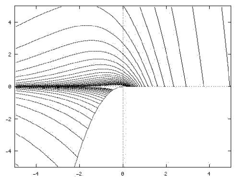
Figure 8: Lines of constant period $T=1/\Omega$ equidistant with $\Delta T=0.3$ on the parameter plane $(\varepsilon,h)$ for the period-doubling bifurcation ($1:2$ resonance, $\omega=1/2$) with $D=1$

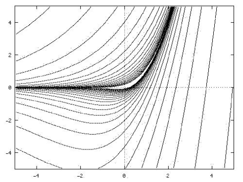
Figure 9: Lines of constant period $T=1/\Omega$ equidistant with $\Delta T=0.3$ on the parameter plane $(\varepsilon,h)$ for the period-doubling bifurcation ($1:2$ resonance, $\omega=1/2$) with $D=-1$

The twist vanishes when

$$0=\frac{\partial T}{\partial h}=\frac{\partial T}{\partial k}\frac{\partial k}{\partial h}\,.$$

The last factor $\partial k/\partial h$ does not vanish for $k\in(0,1)$. In the cases $+2$, $-2$, and $-0c$ it seems to vanish when $k=1/2$. But this implies that $\varepsilon=0$ and the singularity cancels. Therefore it is enough to consider ${\partial T}/{\partial k}=0$. After removing common non-vanishing factors the conditions for vanishing twist are $V_{i}(k)=0$, $i=1,2,3$ where

$$+2,-2,-0c: V_{1}(k)= (1-2k^{2})E(k)-(1-k^{2})K(k),$$ (23)

$$+4,-0i: V_{2}(k)= \left(1-\frac{k^{2}}{2}\right)E(k)-(1-k^{2})K(k),$$ (24)

$$-4: V_{3}(k)= (1+k^{2})E(k)-(1-k^{2})K(k)\,.$$ (25)

The three equalities $V_{i}(k)=0$, $i=1,2,3$ are never satisfied on the range $k\in(0,1)$. Obviously $V_{i}(0)=0$, while $V_{i}(1)=-1,1/2,2$ for $i=1,2,3$, respectively. So we need to show that $V_{1}$ is negative and $V_{2}$, $V_{3}$ are positive for $k\in(0,1)$. Differentiating $V_{1}$ and $V_{2}$ gives the simple results

$$V^{\prime}_{2}(k)= -\frac{3}{2}k(K(k)-E(k))$$ (26)

$$V^{\prime}_{3}(k)= -3kE(k)$$ (27)

In the last case $V^{\prime}_{3}(k)$ is obviously non-positive, so that the twist in the case $-4$ is a monotone funtion rising from 0, hence it is nonzero. Similarly also $V^{\prime}_{2}(k)$ is non-positive, which follows from the well known inequality $K(k)>E(k)$. The first function $V_{1}(k)$ is negative on $(0,1)$, but not monotone. Rewriting it as

$$V_{1}(k)=(1-k^{2})(E(k)-K(k))-k^{2}E(k)<0$$

the inequality is clear because both terms are negative for $k\in(0,1)$. Therefore the twist never vanishes in a neighborhood of the period doubling bifurcation.

The relation between the cases $D=\pm 1$ is interesting. The main observation is that changing the sign of $D$ and $\varepsilon$ inverts the overall sign of the potential $V(x;D,\varepsilon)=Dx^{4}/4+2\varepsilon x^{2}$. Therefore changing the signs of $D$, $\varepsilon$, and $h$ leaves the roots of $P_{4}$ invariant. By this mapping the regions in parameter space with the same numbers of real roots are mapped into each other. The integration path does change in a less trivial way. The integration needs to be taken over the positive intervals of $P_{4}$ on the real axis. Changing the sings of $D$, $\varepsilon$, and $h$ does change the sign of $P_{4}$. As a result the periods for $D=1$ are the $\alpha$ cycles of the elliptic curve, while those for $D=-1$ are the $\beta$ cycles. Hence the period for the case $-4$ can be obtained from that of $+4$ by replacing $K(k)$ by $K^{\prime}(k)=K(\sqrt{1-k^{2}})$. Similarly, the cases $+2$ and $-2$ are mapped into each other.

The obvious symmetry in Figures 8 and 9 with respect to changing the sign of $h$ is related to the fact that changing the sign of $D$ and $h$ leaves the ratio $r$, and therefore also the corresponding modulus $k^{2}$, invariant. This means that the level lines in region $+2$ and $-2$ can be obtained from each other by reflection on the $h=0$ axis. In a similar way the regions $+4$ and $-0i$ have the same rotation number.

The period doubling could have been treated in a scaled version with only one essential parameter $\delta=h/\varepsilon^{2}$. However, the presentation seems more transparent in the unscaled version. Similar to the case of the saddle-centre bifurcation the modulus $k^{2}$ of the elliptic integral for the period is constant on the parabolas $h=\delta\varepsilon^{2}$. Again dependence on the parameters on these curves is simply algebraic, as before through $|\varepsilon|^{1/4}$. The value of the modulus is not defined at the origin, but depends on the parabola on which it is approached. But in any case, there are no twistless tori near the origin in this bifurcation.

4 Universality

A major problem in our approach seems to be that the invariant twistless tori in the normal form are not compact. The normal form is obtained from an expansion near the bifurcation point, and is therefore local in phase space and local in the parameter. How can the rotation number of a non-local invariant torus be determined from this local normal form? To answer this question higher order terms need to be considered in the Hamiltonian. The Poincaré map near the bifurcation can be described by the time $1$ map of the Hamiltonian

$$\tilde{H}(u,v,t;\varepsilon)=H(u,v;\varepsilon)+G(u;\varepsilon)+R(u,v,t;\varepsilon)\,.$$

The remainder terms $R$ containing the periodic time dependence can be made arbitrarily small, but they cannot in general be removed while retaining a non-zero radius of convergence of the normal form. The first term $H$ is the normal form analysed in the previous chapters. We will concentrate on the saddle-centre case (2), but similar remarks apply to (17). The invariant tori near the origin for $\varepsilon>0$ of $H$ are not compact. The higher order terms in $G$ can compactify them. The results about vanishing twist can be applied when $G$ does compactify these curves. However, the precise form of $G$ does not matter. Under the compactness assumption KAM theory can be applied to $H+G$, where $R$ is the perturbation. Many of the invariant tori of $H+G$ will persist. In particular a twistless invariant torus of $H+G$ will persist if it is sufficiently irrational. The curve (14) in the parameter plane therefore does not have invariant twistless tori in its perimage for every point, instead just for a cantorset of points. This is well understood. The main issue in this section is to understand the effect of adding $G$ to $H$. For small $\varepsilon$ the essential contribution to the diverging period comes from the dynamics near the origin, while the dynamics on the invariant torus away from the origin has finite period. This is why the local normal form can give a statement about the dynamics on a non-local invariant torus near the bifurcation point. In particular we will now show that the curve of vanishing twist that was found to be emanating from the cusp of the saddle-centre bifurcation has a universal shape sufficiently close to the cusp singularity. In particular this means that the constant $\gamma_{0}$ that determines the shape of the curve of twistless tori in relation to the curve of critical values of the unstable orbits has the universal value $\gamma_{0}\approx 0.91522$. Quantities derived from $\gamma_{0}$, like $z_{0}$ and the coefficients in (16), are accordingly also universal. Our calculation will show that the value of $\gamma_{0}$ is not influenced by the higher order terms $G$ in the Hamiltonian. Moreover, the following argument also shows that integrating the non-compact invariant torus up to $v=\pm\infty$ does not introduce and additional error.

Let the high-order truncated normal form Hamiltonian be

$$H(u,v;\varepsilon)=\frac{1}{2}v^{2}+\frac{1}{3}u^{3}+\varepsilon u+G(u,\varepsilon)$$

where $G(0,\varepsilon)=0$ and $G(u,0)=0$ is an analytic function. It is not necessary to assume that the higher order terms in $G$ depend on $v$ also, see e.g. [8], but even with such a dependence a slightly modified argument would work. As already explained, it is now assumed that $G(u,\varepsilon)$ is such that the invariant curves near the origin for $\varepsilon>0$ are compact.

Hamiltons equation for $u$ reads $\dot{u}=v$ as before. The period is obtained by solving $H(u,v;\varepsilon)=h$ for $v=v(u;h,\varepsilon)$ and then by integrating

$$T(h,\varepsilon)=\oint\frac{{\rm d}u}{v(u;h,\varepsilon)}\,.$$

The idea is to split the integral into two parts; one part near the origin, where the main contribution originates, and the rest, which is called $T_{3}$. In addition the singular integral near the origin is split again into two parts, $T_{1}$ which has the same integrand as in the previous calculation with $G=0$, and a correction $T_{2}$ which contains the contribution from $G$. The integral $T_{1}$ will be the most singular, $T_{2}$ is mildly singular, and $T_{3}$ is regular. For sufficiently small $\varepsilon$ then $T_{1}$ dominates and the previous result is recovered.

To achieve the splitting into $T_{1}$ and $T_{2}$ the multiplicative structure of the original inegrand has to be recovered. Solving $H=h$ for $v$ and inserting into $\dot{u}$ gives

$$\dot{u}^{2}=v(u;h,\varepsilon)^{2}=Q_{0}(u;h,\varepsilon)\hat{Q}(u;h,\varepsilon)$$

where $\hat{Q}=1+O(u)$ when $|u|\leq C\leq 1$ for some fixed constant $C$, and $Q_{0}$ is a polynomial of degree 3 in $u$ whose zeroes approach those of the original case with $G=0$ when $\varepsilon\to 0$. Denote by $\gamma_{C}$ the part of $H(u,v;\varepsilon)=h$ for which $|u|<C$, and $\bar{\gamma}_{C}$ the rest of the invariant torus. Then the period integral can be split as

$$T(h,\varepsilon)= \int_{\gamma_{C}}\frac{{\mathrm{d}}u}{\sqrt{Q(u,\varepsilon,h)}}+\int_{\bar{\gamma}_{C}}\frac{{\mathrm{d}}u}{\sqrt{Q(u,\varepsilon,h)}}$$ (28)

$$= \int_{\gamma_{C}}\frac{{\mathrm{d}}u}{\sqrt{Q_{0}(u,\varepsilon,h)}}+\int_{\gamma_{C}}\frac{{\hat{Q}(u,h,\varepsilon)}^{-1/2}-1}{\sqrt{Q_{0}(u,\varepsilon,h)}}\,{\mathrm{d}}u+\int_{\bar{\gamma}_{C}}\frac{{\mathrm{d}}u}{\sqrt{Q(u,\varepsilon,h)}}$$ (29)

$$= T_{1}+T_{2}+T_{3}\,.$$ (30)

Now $T_{3}$ is regular, and gives a bounded contribution, so we can ignore it. The integral $T_{1}$ is singular in the limit $h,\varepsilon\to 0$. $T_{2}$ is less singular, and in particular bounded, because the numerator goes to zero in this limit. So we only need to show that $T_{1}$ approaches the complete integral when $\varepsilon\to 0$. The integral is

$$T_{1}(h,\varepsilon)=\frac{4\sqrt{3/2}}{r^{1/2}}F(\phi,k),\quad\phi=2\arctan\sqrt{\frac{u_{0}+C}{r}}\,,$$

where $u_{0}$ is the real root, $\zeta$ is the complex roots of $Q_{0}$, and $r$ and $k$ are as before,

$$r=\sqrt{2u_{0}^{2}+|\zeta|^{2}},\quad 2k^{2}=1+\frac{3u_{0}}{2r}\,.$$

The integral $T_{1}$ does not diverge because of the modulus $k^{2}\to 1$, but because in the prefactor $r\to 0$. In fact, we already observed that the modulus $k^{2}\leq(\sqrt{3}+2)/4<1$ inside the first quadrant $\varepsilon\geq 0,h>0$. The behaviour of $r$ for small $\varepsilon$ is obtained from

$$r^{2}=\frac{3}{2}u_{0}\sqrt{1+\alpha^{2}}=D(\gamma)\varepsilon^{1/4}\,.$$

This shows that $\phi\to\pi$, and the integral approaches the complete integral with the same modulus $k(\gamma)$ as before. Therefore even though $T_{1}$ is an incomplete integral, in the limit of small $\varepsilon$ its value approaches that of the complete integral $T(h,\varepsilon)$, which diverges. Since the other integrals $T_{2}$ and $T_{3}$ are finite the analysis obtained from the complete integral over the non-compact curve of $H(u,v;\varepsilon)$ with $G=0$ therefore correctly describes the behaviour of the rotation number of the compact invariant curve obtained when $G\not=0$.

5 Example: Hénon Map

$\varepsilon$ $u\varepsilon^{-1/2}$ $\Omega\varepsilon^{-1/4}$ 0.1 0.027 0.28314 0.01 0.328 0.17278 0.001 0.478 0.14656 0.0001 0.528 0.14008 0.00001 0.545 0.13823 0.000001 0.550 0.13767

Table 1: Numerically measured position $u$ and rotation number $\Omega$ of the twistless curve for the three times iterated Hénon map with parameter $k=1-\varepsilon$.

The Hénon map in the area preserving case,

$$(x^{\prime},y^{\prime})=(y-k+x^{2},-x)\,,$$

illustrates the above. There are saddle-centre bifurcations in the Hénon map for which the invariant tori for $\varepsilon>0$ are not compact, and hence the vanishing twist cannot be observed. This applies to the initial bifurcation at $k=-1$ that creates the pair of fixed points, and also to many saddle-centre bifurcations that occur for $k>4$. However for $k=1$ a pair of period 3 orbits is created at the origin in a saddle-centre bifurcation of the third iterate of the map, and the corresponding invariant tori are compact. One of the period three points is located on the symmetry line $x=-y$. In new coordinates $(u,v)=(x,y+x)$ the third iterate of the map expanded near the origin with parameter $k=1-\varepsilon$ is

$$(u^{\prime},v^{\prime})=\left((u-v)(1+4v),v+\varepsilon+(u^{2}-2uv+3v^{2})\right)+O(u^{3},v^{3},\sqrt{|\varepsilon|}^{3})\,.$$

The (exact) location of the fixed points is $(u,v)=(\pm\sqrt{-\varepsilon},0)$, with trace of the Jacobian $2\mp 2\sqrt{-\varepsilon}+8\varepsilon\mp 8(-\varepsilon)^{3/2}$ so that the (approximate) multiplier is $\mu\approx 1+{\mathrm{i}}\sqrt{2}(-\varepsilon)^{1/4}$ and $\bar{\mu}$ for the fixed point at $u=\sqrt{-\varepsilon}$. The corresponding rotation number $\omega$ of the elliptic fixed point is obtained from $\mu=\exp(2\pi{\mathrm{i}}\omega)$, so that $\omega=(-\varepsilon)^{1/4}/(\sqrt{2}\pi)$. For small positive $\varepsilon$ the Hénon map possesses compact invariant curves near the origin. A higher order normal form would give a $G$ that describes these invariant curves. The Hénon map is non-integrable, so that only sufficiently irrational invariant curves of the (high order) normal form will exist in the Hénon map. For the situation under consideration numerical experiments show that many of these invariant curves do exist.

Considering the third iterate of the Hénon map turns the pair of period three orbits into three pairs of fixed points with heteroclinic connections. In the normal form there is only one pair of fixed points, and the unstable fixed point has a homoclinic connection. To match the prediction in the case of more than one unstable fixed point the period and hence rotation number must be calculated for the heteroclinic connection. For $\varepsilon>0$ there are invariant tori on which the dynamics becomes slow near the three points that are close to the three bifurcation points of the third iterate of the map. Hence the rotation number for the third iterate of the map between two successive such points gives the correct rotation number. The results together with the position of the twistless curve are shown in table 1. The values shown converge to the predicted values given in (15) and (16), however, fairly small $\varepsilon$ are needed to see this. The convergence to the true value $0.1374244...$ occurs approximately as $\tfrac{1}{2}\varepsilon^{5/4}$.

References

- [1] V. I. Arnold. Mathematical Methods of Classical Mechanics, volume 60 of Graduate Texts in Mathematics. Springer, Berlin, 1978.
- [2] D. del Castillo-Negrette, J.M. Greene, and P.J. Morrison. Area preserving nontwist maps: Periodic orbits and transition to chaos. Physica D, 91(1):1–23, 1996.
- [3] A. Delshams and R. de la Llave. KAM theory and a partial justification of Greene’s criterion for nontwist maps. SIAM J. Math. Anal., 31(6):1235–1269 (electronic), 2000.
- [4] H. R. Dullin and J. D. Meiss. Twist singularities for symplectic maps. Chaos, 13(1):1–16, 2003.
- [5] H. R. Dullin, J. D. Meiss, and D. G. Sterling. Generic twistless bifurcations. Nonlinearity, 13:203–224, 2000.
- [6] J. E. Howard and J. Humpherys. Nonmonotonic twist maps. Physica D, 80(3):256–276, 1995.
- [7] J.E. Howard and S.M. Hohs. Stochasticity and reconnection in hamiltonian systems. Physical Review A, 29:418, 1984.
- [8] K. R. Meyer and G. R. Hall. Introduction to Hamiltonian Dynamical Systems and the N-Body Problem. Springer, Berlin, 1992.
- [9] R. Moeckel. Generic bifurcations of the twist coefficient. Ergodic Theory Dynam. Systems, 10(1):185–195, 1990.
- [10] D. A. Sadovskii and J. B. Delos. Bifurcation of the periodic orbits of hamiltonian systems: An analysis using normal form theory. Phys. Rev. E, 54:2033–2070, 1996.
- [11] C.L. Siegel and J.K. Moser. Lectures on Celestial Mechanics. Classics in Mathematics. Springer-Verlag, New York, 1971.
- [12] C. Simó. Invariant curves of analytic perturbed nontwist area preserving maps. Regular & Chaotic Dynamics, 3:180–195, 1998.
- [13] J. P. Van der Weele and T. P. Valkering. The birth process of periodic orbits in nontwist maps. Physica A, 169(1):42–72, 1990.