A Toy Model of Flying Snake’s Glide

Abstract

We have developed a toy model of flying snake’s glide [J.J. Socha, Nature 418 (2002) 603.] by modifying a model for a falling paper. We have found that asymmetric oscillation is a key about why snake can glide. Further investigation for snake’s glide will provide us details about how it can glide without a wing.

1 Introduction

Biological fluid mechanics[1, 2] is recently an interesting field. It is unclear why dolphins or tuna fishes can swim so rapidly and why small insects like flies or bees can get large enough lift force. However a flyingsnake[3] is stranger than them in the light of fluid mechanics. Although it does not have anything like wings, it can glide with constant falling speed. This means it can produce at least some lift force which cancels downward gravity. Here we have shown how it can glide without wings using the toy model [4] which is originally proposed for explaining the behaviour of a falling paper. A falling paper exhibits several behaviour ranging from a simple falling to a periodic rotation[5]. However, there are no directional gliding motions which the flyingsnake can have. We have found asymmetric oscillating motion can induce a gliding motion. Probably this is the reason why the flyingsnake must oscillate when it glides.

When the flying snake would like to glide[3], it jumps up from some higher location. After some short transient time period, it starts to glide. While gliding, it shapes on horizontal plane a S letter. Furthermore head-to-tail distance oscillates periodically. It seems to get lift force without doing anything special other than that. It is the rather difficult task to understand by fluid mechanics this mechanism. Fluid around a falling snake is disturbed violently and its spatio-temporal patterns are very complicated, probably something like that called turbulence appears. It is difficult not only to understand such complicated spatio-temporal patterns but also to simulate them numerically.

2 A Falling Paper Model and its Modification for Flying Snake

Tanabe-Kaneko model[4] can reproduce qualitatively the behaviour of a falling paper; chaotic or periodic rotations, chaotic or periodic flutterings and a simple falling, although there are some criticisms to this model[6]. In Tanebe-Kaneko model, a falling paper has only three state variables; a horizontal velocity, a vertical velocity, and an angle of inclination of paper. This means, a falling paper is modeled as a line segment which goes down in vertical plane. Thus its motion is restricted to be within two dimensions. External forces are a gravity, a viscosity force and a lift. Although the later two forces are complicated functions of the velocity field of the surrounding fluid, Tanabe and Kaneko assume they depend upon only a horizontal velocity, a vertical velocity and an angle of inclination of paper. In this study we employ this model in order to describe a flying snake’s gliding motion.

In order to model snake’s gliding with this model, we have assumed that

1. Neither viscosity force nor lift changes due to oscillations. Viscosity force is mainly dependent upon level cross-section area on which snake shapes S letter. This area does not change due to oscillation. Lift mainly depends upon snake’s volume, which is conserved during oscillation.

2. Inertia moment is strongly dependent upon oscillation because head-to-tail distance is proportional to its gyration radius whose squared value is proportional to inertia moment.

Except for those mentioned above, snake is regarded as a falling paper.

When snake oscillates, the distance $d$ between head and tail has time dependence as $d(t)$. Other than making inertia moment dependent upon time, we do not modify Tanabe-Kaneko model at all. As a result, our model for flying snake is[7]

$$\begin{split}\dot{u}&=-(k_{\perp}\sin^{2}\theta+k_{\parallel}\cos^{2}\theta)u+(k_{\perp}-k_{\parallel})\sin\theta\cos\theta v\mp\pi\rho V^{2}\cos(\alpha+\theta)\cos\alpha,\\ \dot{v}&=(k_{\perp}-k_{\parallel})\sin\theta\cos\theta u-(k_{\perp}\cos^{2}\theta+k_{\parallel}\sin^{2}\theta)v\pm\pi\rho V^{2}\cos(\alpha+\theta)\sin\alpha-g,\\ \dot{\omega}&=-k_{\perp}\omega-(3\pi\rho V^{2}/d(t))\cos(\alpha+\theta)\sin(\alpha+\theta),\end{split}$$ (1)

where fluid density ratio $\rho$ is $\rho_{f}\ell_{c}/m_{p}$, $\rho_{f}$ is fluid density, $m_{p}$ and $\ell_{c}$ are mass and horizontal size of snake respectively. As mentioned above, $\ell_{c}$ does not change with oscillation but takes constant value. $u$ and $v$ are horizontal velocity and vertical one, $\omega$ is the angular velocity on the vertical plane. $k_{\perp}$ ($k_{\parallel}$) is the friction coefficients along the perpendicular (parallel) direction to a plane on which a snake shapes a S letter. $\theta$ is incline angle of this plane. $\alpha\equiv\arctan(u/v)$ and $V=\sqrt{u^{2}+v^{2}}$.

3 Results

We have tried to find $d(t)$ which induces the gliding motion which Tanabe-Kaneko original model lacks. First of all, we employ simple harmonic motion as $d(t)$. It cannot induce gliding motions at all, although we check any possibilities that original model exhibits any motions. Thus we tried other oscillating motions. After several trials and errors, we found three cases which can produce gliding motion. These three $d(t)$s are

$$d(t)=\left\{\begin{array}[]{l}0.3(1+\sin\omega_{0}t)^{2}+0.7,\\ \exp(-1-1.3\sin\omega_{0}t),\\ 1/[1+0.5\sin\omega_{0}t].\end{array}\right.$$

In the case of all of these three, $d(t)$ oscillates around 1.0. When $d(t)$ takes the constant values, this corresponds to original model of a falling paper. Also, as long as we tried, gliding motion can take place only when $d(t)$ oscillates around the value with which a periodic fluttering occurs in the original model.

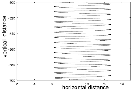
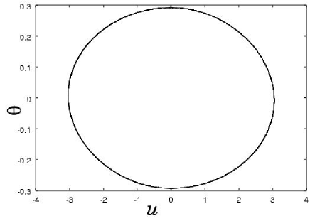
Figure 1: Left: trajectory of periodic fluttering of a falling paper reproduced by Tanabe-Kaneko model ($d(t)=1$). Right: $\theta(t)$ as a function of $u(t)$. Their relation is the same as that between the velocity and the coordinates observed when harmonic motion takes place.

In Figure 1, we show periodic fluttering of a falling paper. We also show $\theta(t)$ as a function of $u(t)$. Due to the symmetric motion, their relation is also symmetric and is nearly equal to that between the velocity and the coordinates observed when a harmonic motion takes place.

Now in order to simulate snake case, we have to consider the time dependence of $d(t)$.

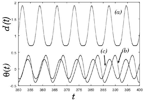
Figure 2: (a) $d(t)=0.3(1+\sin\omega_{0}t)^{2}+0.7$, $\omega_{0}=0.9$ (b) $\theta(t)$ when $d(t)=1$. Its time dependence is almost sinusoidal because paper flutters periodically. (c) $\theta(t)$ when $d(t)$ varies as shown in (a). Due to the oscillation, period of fluttering becomes close to that of oscillation.

In Figure 2(a), we show $d(t)$ as a function of $t$. This aymmetric oscillation has turned out to be important in order to induce gliding motion. This is the reason why simple harmonic motion cannot induce gliding motion. Due to this asymmetry, as $d(t)$ becomes larger, velocity of oscillation becomes higher, in contrast to the simple harmonic motion. When oscillation is asymmetric as shown above, $\theta(t)$ can resonate to the oscillation (Figure 2(b)) if $\omega_{0}$ is chosen properly. This means that the period of fluttering is forced close to that of oscillation. Moreover, as shown in Figure 2(c), this resonance violates time reversal symmetry of $\theta(t)$ which $\theta(t)$ for periodic fluttering has. Because of this symmetry breaking, periodic fluttering motion becomes gliding motion although fluttering motion does not vanish completely (See Figure 3).

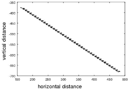
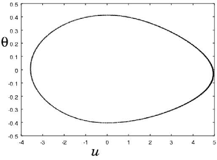
Figure 3: Left: A trajectory in vertical plane. Right: $\theta(t)$ vs $u(t)$ for the left figure. The symmetry seen in the motion without oscillation (Figure 1) has vanishes.

For a long period, a falling paper keeps constant velocity and constant angle $\theta(t)$ as if flying snake keeps them[3]. Also in Figure 3, we show $\theta(t)$ as a function of $u(t)$. Since asymmetric motion of $\theta(t)$ results in that of $u(t)$, in average a falling paper can move along one direction. This is the reason why oscillation causes gliding motion, i.e. a falling along one direction.

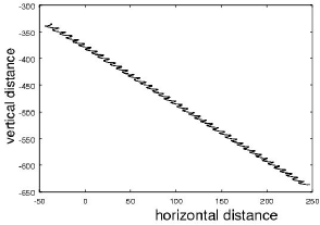
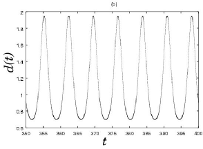
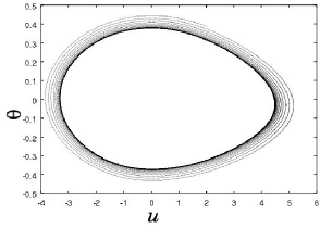
Figure 4: Left:$d(t)=\exp(-1-1.3\sin\omega_{0}t)$, $\omega_{0}=0.9$ Center: A trajectory in vertical plane. Right: $\theta(t)$ vs $u(t)$ for the center figure.

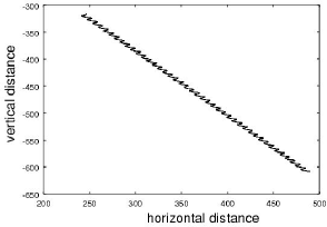
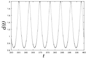
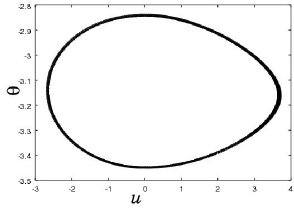
Figure 5: Left:$d(t)=1/[1+0.5\sin\omega_{0}t]$, $\omega_{0}=0.9$ Center: A trajectory in vertical plane. Right: $\theta(t)$ vs $u(t)$ for the center figure.

For the remaining two cases, we also show trajectory, $d(t)$, and $\theta(t)$ vs $u(t)$ (Figures 4 and 5). In order to induce gliding motion, for these two cases, $d(t)$ must have time dependencies similar to that of the first case, too. Although all of them induces the motions along the one direction, there are some differences among these three cases. For the first case, $\theta-u$ plot shows very narrow band, which means gliding motion is very periodic. On the other hand, for the second case, $\theta-u$ plot tends to converge to the periodic motion very slowly. And for the third case, $\theta-u$ plot shows relatively broader band, this means simple periodic motion is modulated by slower periodic motion.

In spite of these minor differences, their global behaviours are very similar. Thus, there should exist much more such possibilities of $d(t)$ that cause gliding motion. Of course, $d(t)$ cannot take so different shapes from the above cases. As long as we tried, only these shapes can induce gliding motion. Probably, a flying snake would have found such very rare possibilities during its evolutions, because it has much more time for trial than we spent.

It is also a problem that we cannot stop fluttering motion completely. However, a flying snake can choose any other much more complicated time dependence of $d(t)$ Further detailed investigation of snake’s motion will tell us which $d(t)$ can induce a simple gliding motion that is not accompanied with the fluttering.

4 Sensitivities to the detailed parameter values or the forms of the function $d(t)$

Finally, we would like to comment on sensitivities to the detailed parameter values or the forms of the function $d(t)$. Once we fix all parameter values other than those included in $d(t)$, we can change the functional form of $d(t)$ very little. For example, if we slightly change the value $0.3$ in the form of $d(t)=0.3(1+\sin\omega_{0}t)^{2}+0.7$, the directional gliding motion disappears quickly. Actually speaking, three $d(t)$s mentioned above are tuned so that they have almost equal time dependency. Thus, we believe that this specific form is very important.

Also, the condition for the directional gliding motion is asymmetry. As mentioned above, asymmetry in $d(t)$ results in that in velocity which causes directional motions. For example, if we employ a normal sinusoidal motion

$$d(t)=0.6\sin\omega_{0}t+1.3,\omega_{0}=0.9,$$

there is not any asymmetry in velocity, thus directional gliding motions cannot appear (Fig. 6).

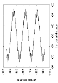
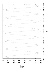
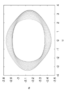
Figure 6: Left:$d(t)=0.6\sin\omega_{0}t+1.3$, $\omega_{0}=0.9$ Center: A trajectory in vertical plane. Right: $\theta(t)$ vs $u(t)$ for the center figure.

In spite of the fact that $d(t)$ is tuned so that its functional form is close to those of three $d(t)$s excluding the asymmetry, directional motion cannot occur. Thus it is clear that asymmetry is the most important factor.

It is also easily understood that the direction of motion is determined by the initial condition. Asymmetry in $d(t)$ cannot decide in which direction symmetry is broken. This depends upon how the snake starts to fly.

References

- [1] C.P. Ellington and T.J. Pedley, (eds) Biological Fluid Dynamics (Cambrige, UK,1995)
- [2] L.J. Fauci and S. Gueron, Computational Modeling in Biological Fluid Dynamics (Springer-Verlag, New York, 2001)
- [3] J.J. Socha, Nature 418 (2002) 603.
- [4] Y. Tanabe and K. Kaneko, Phys. Rev. Lett. 73 (1994) 1372.
- [5] S. B. Field, M. Klaus, M. G. Moore and F. Nori, Nature 388 (1997) 252.
- [6] L. Mahadevan, H. Aref and S. W. Jones, Phys. Rev. Lett. 75 (1995) 1420.
- [7] We solve the equation of motion (1) using the forth order Runge-Kutta method. Parameters used are as follows: , and . Initial conditions are . Under these conditions, original model (i.e. ) induces periodic flattering motion.