Decay of metastable patterns for the Rosensweig instability: revisiting the dispersion relation

Abstract

The decay of metastable patterns in the form of magnetic liquid ridges is studied in the frame of a linear stability analysis where the ridges are the most unstable linear pattern of the Rosensweig instability. The analysis of the corresponding dispersion relation reveals that different sets of solutions exist. Two of them are associated with an oscillatory and a pure exponential decay, respectively.

1. Introduction

The most well known phenomenon of pattern formation in magnetic fluids is the Rosensweig or normal field instability. This instability can be observed for a horizontal layer of magnetic fluid (MF) with a free surface with air above. Beyond a certain threshold $B_{\rm c}$ of a vertically applied homogenous magnetic induction, the surface becomes unstable and a stable pattern of peaks develops [1]. That final pattern, resulting from nonlinear interactions, is one possible state towards which the preceding most unstable linear pattern of liquid ridges can develop if a supercritical induction $B_{\rm sup}\!>\!B_{\rm c}$ is abided [2]. The other possible state results from the decay of the liquid ridges towards the flat surface if the induction is switched from a supercritical to a subcritical value $B_{\rm sub}$ [3]. With these two possible final states, the most unstable linear pattern can be considered as a metastable pattern formed by magnetic liquid ridges.

That ridges were studied in [4, 3] by means of an experimental set-up in which the magnetic induction was jumplike increased from a start value of $B_{\rm 0}<B_{\rm c}$ to $B_{\rm sup}$ [4] and after a short time delay jumplike decreased from $B_{\rm sup}$ to $B_{\rm sub}$[3]. The jumplike change of the magnetic induction allows to apply the linear stability theory, where the magnetic induction is assumed to be instantly present. Consequently, the quantitative agreement between measured and calculated data is very good for the wave number of the linearly most unstable ridges [4] and for the propagation velocity as well as the oscillation frequency during the decay of the ridges [3]. The calculation of the latter two quantities disclosed new features of the dispersion relation which will be revisited and analysed in the next section.

2. Analysis of the dispersion relation

A horizontally unbounded layer of an incompressible, nonconducting, and viscous MF of infinite thickness and constant density $\rho$ is considered. The MF has a free surface with air above, where the basic state is that of a nondeformed surface. The dispersion relation for small disturbances from the basic state is given by [5]

$$\left(1-{i\omega\over 2\nu q^{2}}\right)^{2}+{1\over 4\rho\nu^{2}q^{4}}\left[\rho gq+\sigma q^{3}-{(\mu_{r}-1)^{2}B^{2}q^{2}\over(\mu_{r}+1)\mu_{0}\mu_{r}}\right]=\sqrt{1-{i\omega\over\nu q^{2}}}\;,$$ (1)

where $g$ is the gravity acceleration, $\nu$ the kinematic viscosity of the MF, $\sigma$ its surface tension with air, $\mu_{r}$ its relative permeability, $B$ the absolute value of the external magnetic induction, and $\mu_{0}$ the permeability of vacuum. For the dispersion relation (1), the small disturbances were decomposed into normal modes, i.e. they are proportional to $\exp[-i(\omega\,t\!-\!{\bf q}\,{\bf r})]$. ${\bf r}\!=\!(x,y)$ is the planar space vector, ${\bf q}\!=\!(q_{x},q_{y})$ the wave vector, and $q\!=\!|{\bf q}|$ denotes the wave number. With $\omega\!=\!\omega_{1}+i\omega_{2}$ the real part of $-i\omega$, $\omega_{2}$, is called the growth rate and defines whether the disturbances will grow ($\omega_{2}>0$) or decay ($\omega_{2}<0$). The absolute value of the imaginary part of $-i\omega$, $|\omega_{1}|$, gives the angular frequency of the oscillation if $\omega_{1}$ is different from zero. The critical induction for the onset of the Rosensweig instability at $\omega=0$ is $B_{c}^{2}=2\mu_{0}\mu_{r}(\mu_{r}+1)\sqrt{\rho\sigma g}(\mu_{r}-1)^{-2}$ [1].

Figure 1 shows for the reasons of clarity one solution of the dispersion relation for a supercritical induction $B_{{\rm sup}}=1.05B_{c}$ (thick solid line) and for a subcritical induction $B_{{\rm sub}}=0.96B_{c}$ (thick dashed line). In the supercritical case one can conclude from ${\rm Re}[\omega^{2}(q_{\rm m},B_{{\rm sup}})]=\omega_{{\rm 1,m}}^{2}-\omega_{{\rm 2,m}}^{2}<0$ and ${\rm Im}[\omega^{2}(q_{\rm m},B_{{\rm sup}})]=2\omega_{{\rm 1,m}}\,\omega_{{\rm 2,m}}=0$ that a most unstable linear patterns evolves with the maximal growth rate $\omega_{\rm m}=i\omega_{\rm 2,m}$ ($\omega_{\rm 2,m}>0$) and its corresponding wave number $q_{\rm m}$ [thin solid lines in Fig. 1(a)]. In the subcritical case the relations ${\rm Re}[\omega^{2}(q_{\rm m},B_{{\rm sub}})]>0$ and ${\rm Im}[\omega^{2}(q_{\rm m},B_{{\rm sub}})]<0$ [thin dashed lines in Fig. 1(a)(b)] do not allow a simple conclusion on the values of $\omega_{{\rm 1}}$ and $\omega_{{\rm 2}}$. Therefore the classical presentation of $\omega^{2}$ versus $q$ chosen for the analysis of inviscid MFs [8, 7, 6] is only of limited use for the analysis of viscous MFs.

A more meaningful display is the plot of ${\rm Re}(-i\omega)$ and ${\rm Im}(-i\omega)$ versus the subcritical induction for different viscosities (see Fig. 2), where $q_{\rm m}(\nu)$ of the most unstable linear pattern was determined for $B_{\rm sup}=18$ mT. If the fluid is inviscid (dashed lines in Fig. 2), the pattern oscillates below a certain threshold for the subcritical induction, $B_{\rm c,0}[q_{\rm m}(\nu=0),\omega_{2}=0]$ [see Eq. (5)]. Above that threshold the pattern can either decay according to the solution ${\rm Re}(-i\omega)<0$ or can develop towards the most unstable linear pattern belonging to $B_{\rm sub}\!>\!B_{c}$ since ${\rm Re}(-i\omega)>0$ is also a solution.

For a viscous fluid (solid lines in Fig. 2) the behaviour is more complex. A first critical induction, $B_{\rm c,1}$, occurs, where the set of solutions for the dispersion relation (1) changes from two complex solutions to two negative real solutions. [The same transition occurs for the damping of gravity-capillary waves as parameters as the aspect ratio and the so called inverse Reynolds number are varied (see Figs. 4–6 and 8,9 in [9]).] Both real solutions exist until at a second critical induction, $B_{\rm c,2}$, one of them abruptly ends. At a third critical induction, $B_{\rm c,0}$, one of the two negative real solutions changes its sign and becomes positive.

To understand this complex behaviour, the dispersion relation (1) in dimensionless units (indicated by a bar) is analysed in the rearranged form

$$\left(1+{-i\bar{\omega}\over 2\bar{\nu}\bar{q}\,^{2}}\right)^{2}-\sqrt{1+{-i\bar{\omega}\over\bar{\nu}\bar{q}\,^{2}}}={-\bar{q}-\bar{q}\,^{3}+2\bar{B}^{2}\bar{q}^{2}\over 4\bar{\nu}^{2}\bar{q}^{4}}\;.$$ (2)

All lengths were scaled with $[\sigma/(\rho\,g)]^{1/2}$, the time with $\sigma^{1/4}/(g^{3/4}\rho^{1/4})$, the viscosity with $\sigma^{3/4}/(g^{1/4}\rho^{3/4})$, and the induction with $B_{c}$. Equation (2) reveals that whatever value $\bar{\omega}\in{\mathbb{C}}$ has, the left hand side of Eq. (2) has to be real because the right hand side of Eq. (2) is always real since $(\bar{q},\bar{\nu},\bar{B})\in{\mathbb{R}}$. That condition together with the mixing of real and complex quantities in Eq. (2) is essential to understand the above described appearance of different sets of solutions. As long as $B_{\rm sub}\geq B_{\rm c,1}$ all solutions of the dispersion relation with $q=q_{m}$ are real, i.e. $-i\omega=\omega_{2}\in{\mathbb{R}}$ (see Fig. 2). Using this result it follows from Eq. (2) that there is a value $\bar{\omega}_{2}=-\bar{\nu}\bar{q}_{\rm m}^{2}$ beyond which the radicand becomes negative. Since a complex value for the left hand side of Eq. (2) is not allowed, the solution does not exist beyond $\bar{\omega}_{2}=-\bar{\nu}\bar{q}_{\rm m}^{2}$. This corresponds to the point in Fig. 2, where one of the solutions suddenly terminates at $B_{c,2}$. Therefore the second critical induction yields to

$$\bar{B}_{c,2}\bigr{[}\bar{\nu},\bar{q}_{\rm m}(\bar{\nu}),\bar{\omega}_{2}=-\bar{\nu}\bar{q}_{\rm m}^{2}\bigr{]}=\sqrt{{1\over 2}\left({1\over\bar{q}_{\rm m}}+\bar{q}_{\rm m}+\bar{\nu}^{2}\bar{q}_{\rm m}^{2}\right)}\;.$$ (3)

The first critical induction is the minimal induction for which real solutions exist, thus

$$\bar{B}_{c,1}\bigr{[}\bar{\nu},\bar{q}_{\rm m}(\bar{\nu}),\bar{\omega}_{2,\min}\bigr{]}=\sqrt{{1\over 2}\left({1\over\bar{q}_{\rm m}}+\bar{q}_{\rm m}\right)-2\bar{\nu}^{2}\bar{q}_{\rm m}^{2}\left[\sqrt{1+D}-\left(1+{D\over 2}\right)^{2}\right]}$$ (4)

with $\bar{\omega}_{2,\min}=\bar{\nu}\bar{q}_{\rm m}^{2}\,D=(\bar{\nu}\bar{q}_{\rm m}^{2}/36)\bigr{[}-60+(108+12\sqrt{93})^{2/3}+144(108+12\sqrt{93})^{-2/3}\bigr{]}$. Finally, the third critical induction is defined by $\bar{\omega}_{2}=0$ which leads to

$$\bar{B}_{c,0}\bigr{[}\bar{q}_{\rm m}(\bar{\nu}),\bar{\omega}_{2}=0\bigr{]}=\sqrt{{1\over 2}\left({1\over\bar{q}_{\rm m}}+\bar{q}_{\rm m}\right)}\;.$$ (5)

At a closer inspection of Eqs. (3-5) one realizes that the three thresholds follow the relation $\bar{B}_{c,1}\leq\bar{B}_{c,0}\leq\bar{B}_{c,2}$. Their dependence on the viscosity of the magnetic fluid will be studied in the next section.

3. Results and discussion

The behaviour of the three above defined thresholds on the viscosity is studied, where all other material parameters are kept constant. The wave number $q_{\rm m}(\nu)$ for the most unstable linear pattern is determined for a supercritical induction of $18$ mT. Figure 3 shows that for viscous MFs four regions with different sets of solutions for the dispersion relation exist. For small subcritical inductions the set of solutions consists of two complex solutions with negative real parts (symbolised by 2C_– in Fig. 3) which is followed by two negative real solutions (2R_–). Passing the threshold $\bar{B}_{c,0}$ (solid line), the set of solutions is formed by one positive and one negative real solution (2R_+-). Only the former solution lasts at high subcritical inductions (1R₊). From Fig. 3 it becomes clear that for low viscous MFs, $\bar{\nu}\leq 0.1$, only an oscillatory decay can be observed [3, 10]. For high viscous MFs it should be possible to observe an oscillatory (2C_–) as well as a pure exponential decay (2R_–) of the pattern. Because for $\bar{\nu}\gtrsim 0.3$ the two thresholds $\bar{B}_{c,1}$ (dashed line) and $\bar{B}_{c,0}$ are well separated and the region 2R_– becomes experimentally accessible.

For a nonmagnetic fluid with the same density and surface tension, a dimensionless viscosity of $\bar{\nu}\simeq 0.9$ is necessary to have a pure exponential decay, i.e. the nonmagnetic fluid has to be considerable more viscous than the magnetic fluid to result in the same behaviour. Another advantage in the use of a MF is that the jumplike increase to $B_{\rm sup}$ is a simple way to prepare just one particular metastable pattern whose decay can be studied.

For inviscid MFs Fig. 3 shows that only two different sets of solutions occur. For subcritical inductions smaller than $\bar{B}_{c,0}(\bar{\nu}=0)$ two pure imaginary solutions (2I) exist. Above that threshold two real solutions with different signs (2R_+-) are found.

This analysis also leads to a better understanding in the case of a supercritical induction, where regions with different sets of solutions should exist, too. Whereas Fig. 1 shows only one particular solution of the dispersion relation (1) for $0\leq q\leq 1200$ m^-1, the two zooms around $q\!\!=\!418.3$ m^-1 [Fig. 4(a)(b)] and $q\!=\!\!1027$ m^-1 [Fig. 4(c)(d)] present all solutions. In contrast to the material parameters for Fig. 2, now the induction is fixed at $B_{\rm sup}\!=\!18$ mT and therefore transitions between different sets of solutions occur at certain wave numbers. The first zoom [Fig. 4(a)(b)] displays that for wave numbers below $q_{\rm c,1}$ two complex solutions exist. Between $q_{\rm c,1}$ and $q_{\rm c,2}$ two real solutions exist and beyond $q_{\rm c,2}$ only one real solution. In a reverse order the different sets of solutions are appearing in the second zoom [Fig. 4(c)(d)]. These features of the dispersion relation have not been realized since only the solution for $q_{\rm m}$ was of interest in [2, 4, 11]. For that particular wave number the dispersion relation has only one real solution which motivates the plot of one solution (thick solid line) in Fig. 1.

To conclude, in the frame of a linear stability analysis the decay of the metastable pattern of magnetic liquid ridges is studied. There are initiated by a jumplike increase of the magnetic induction to a supercritical value whereas the decay is triggered by a jumplike decrease of the induction. The analysis of the dispersion relation according to such a procedure reveals that depending on the value of the subcritical induction different sets of solutions exist (Fig. 2). The regions for these different sets are separated by the three thresholds (3-5) whose dependence on the viscosity is displayed in Fig. 3. Whereas for low viscous MFs an oscillatory decay of the ridges can be observed [3], for high viscous MFs a pure exponential decay should be detectable, too.

• Received 13.12.2002

Figure 1: Dependence of ${\rm Re}(\omega^{2})$ (a) and ${\rm Im}(\omega^{2})$ (b) on the wave number $q$ for a supercritical ($1.05B_{c}$, thick solid line) and a subcritical ($0.96B_{c}$, thick dashed line) induction. The wave number $q_{m}$ of the most unstable linear pattern and the corresponding value $\omega_{m}^{2}$ are indicated by thin solid lines. The solution in the subcritical case for $q_{m}$ is indicated by thin dashed lines. The material parameters for the calculations are $\nu=5.17\cdot 10^{-6}$ m²/s, $\rho=1.16\cdot 10^{3}$ kg/m³, $\sigma=2.65\cdot 10^{-2}$ kg/s², $\mu_{r}\simeq 1.935$, and $B_{c}=16.84$ mT.

Figure 2: Dependence of ${\rm Re}(-i\omega)$ (a) and ${\rm Im}(-i\omega)$ (b) on the subcritical induction $B_{\rm sub}$ for an inviscid MF ($\nu=0$, dashed line) and a viscous MF ($\nu=5.17\cdot 10^{-6}$ m²/s, solid line). For the former fluid two imaginary solutions are replaced by two real solutions with increasing $B_{\rm sub}$. For the latter fluid a region with two complex solutions is followed by a region with two real solutions which is succeeded by a region with one real solution. The three critical inductions $B_{\rm c,0}$, $B_{\rm c,1}$, and $B_{\rm c,2}$ are explained in the text. The remaining material parameters for the calculations are those from Fig. 1 with $q_{\rm m}(\nu)$ determined for $B_{\rm sup}=18$ mT.

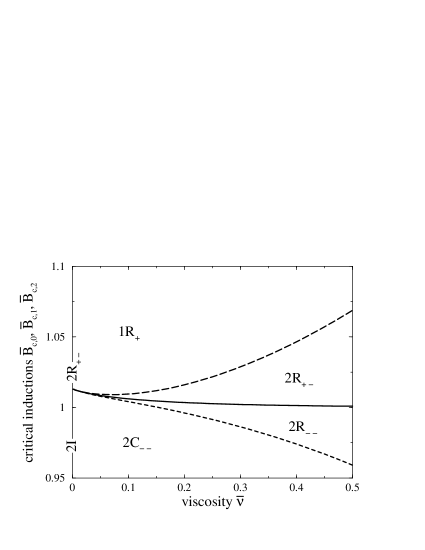
Figure 3: The three critical inductions $\bar{B}_{c,1}$ (dashed line), $\bar{B}_{c,0}$ (solid line), and $\bar{B}_{c,2}$ (long dashed line) versus the dimensionless viscosity $\bar{\nu}$. The regions with different sets of solutions for the dispersion relation are symbolised as follows: 2I – two imaginary solutions, 2C_– – two complex solutions with negative real parts, 2R_+- – two real solutions of different signs, 2R_– – two negative real solutions, 1R₊ – one positive real solution.

Figure 4: All solutions of Eq. (1) for $B=1.05B_{\rm c}$ in the form of ${\rm Re}(\omega^{2})$ (a)(c) and ${\rm Im}(\omega^{2})$ (b)(d) for wave numbers near $q\!\!=\!418.3$ m^-1 (a)(b) and $q\!=\!\!1027$ m^-1 (c)(d). In (a)(b) two complex solutions for $q\leq q_{\rm c,1}$ are followed by two real solutions which exist for $q_{\rm c,1}\leq q\leq q_{\rm c,2}$ (dashed and long dashed lines). For $q_{\rm c,2}\!<\!q$ one real solution (long dashed line) exist. In (c)(d) the order of the different solutions is reverse: first one real solution, then two real solutions and finally two complex solutions. The material parameters are those from Fig. 1. Note the different scales at the axes.

REFERENCES

- [1] M. D. Cowley and R. E. Rosensweig. The interfacial stability of a ferromagnetic fluid. J. Fluid Mech., vol. 30 (1967), no. 4, pp. 671-688.
- [2] A. Lange, B. Reimann, and R. Richter. Wave number of maximal growth in viscous ferrofluids. Magnetohydrodynamics, vol. 37 (2001), no. 3, pp. 261-267.
- [3] B. Reimann, R. Richter, A. Lange, and I. Rehberg. Transient magnetic liquid ridges. Submitted to Phys. Rev. E.
- [4] A. Lange, B. Reimann, and R. Richter. Wave number of maximal growth in viscous magnetic fluids of arbitrary depth. Phys. Rev. E, vol. 61 (2000), no. 5, pp. 5528-5539.
- [5] D. Salin. Wave vector selection in the instability of an interface in a magnetic or electric field. Europhys. Lett., vol. 21 (1993), no. 6, pp. 667–670.
- [6] R. E. Rosensweig. Magnetic fluids. Ann. Rev. Fluid Mech., vol. 19 (1987), pp. 437-463.
- [7] V. G. Bashtovoi, M. S. Krakov and A. G. Reks. Instability of a flat layer of magnetic liquid for supercritical magnetic fields. Magnetohydrodynamics, vol. 21 (1985), no. 1, pp. 14-19.
- [8] R. E. Zelazo and J. R. Melcher. Dynamics and stability of ferrofluids: surface interactions. J. Fluid Mech., vol. 39 (1969), no. 1, pp. 1-24.
- [9] J. A. Nicolás. The viscous damping of capillary-gravity waves in a brimful circular cylinder. Phys. Fluids, vol. 14 (2002), no. 6, pp. 1910-1919.
- [10] The dimensionless viscosity of EMG 909 in [3] is .
- [11] A. Lange. Scaling behaviour of the maximal growth rate in the Rosensweig instability. Europhys. Lett., vol. 55 (2001), no. 3, pp. 327-333.
-