Estimating good discrete partitions from observed data:
symbolic false nearest neighbors

Abstract

A symbolic analysis of observed time series data requires making a discrete partition of a continuous state space containing observations of the dynamics. A particular kind of partition, called “generating”, preserves all dynamical information of a deterministic map in the symbolic representation, but such partitions are not obvious beyond one dimension, and existing methods to find them require significant knowledge of the dynamical evolution operator or the spectrum of unstable periodic orbits. We introduce a statistic and algorithm to refine empirical partitions for symbolic state reconstruction. This method optimizes an essential property of a generating partition: avoiding topological degeneracies. It requires only the observed time series and is sensible even in the presence of noise when no truly generating partition is possible. Because of its resemblance to a geometrical statistic frequently used for reconstructing valid time-delay embeddings, we call the algorithm “symbolic false nearest neighbors”.

Why might one want to represent observed time series of dynamical systems as sequences of low-precision discrete symbols? In this representation, there are often interesting techniques—often (but not exclusively) derived from information theory and its associated technology—which may illuminate data in novel ways symbolictimeseriesanalysis . The initial step for all these methods requires making a partition: a coloring of the state space reconstruction , ${\bf x}\in R^{d}$, into non-overlapping regions and associated symbols so that any ${\bf x}$ is assigned a unique symbol $s$ in a discrete alphabet. The symbol may be represented as an integer in the set ${0,1,\ldots A-1}$. A partition ${\cal P}$ defines a discretization of the observed sequence ${\bf x}_{i},i=1\ldots N$ into a symbolic sequence, $s_{i},i=1\ldots N$.

What partitions are “good”? Which discretizations retain the full structure of the original dynamics in the ${\bf x}$ space in the sequence of symbols? Unfortunately, the situation is unlike the remarkable time-delay embedding method for continuous dynamics: simple partitions are not generically satisfactory. The mathematics of symbolic dynamics specifies what we want: a “generating partition” (GP), where symbolic orbits uniquely identify one continuous space orbit, and thus the symbolic dynamics is fully equivalent to the continuous space dynamics.

Unfortunately there is no satisfactory mathematical theory about how to find a GP as a general procedure (except for one dimensional dynamics ($d=1$), where partitioning at the critical points works). Are the ad-hoc partitions often used still satisfactory? Unfortunately they are often not so. Bollt et al bollt examined the degradation in the symbolic dynamics which results from the frequently used “histogram partition”, as opposed to a GP. A less optimal partition will induce improper projections or degeneracies, where a given symbolic segment may correspond to more than one topologically distinct state space orbit. This resulted in finding the wrong topological entropy. Chaotic communication with symbolic targeting works most satisfactorily knowing a GP, because then the transmitted symbolic message may be directly mapped into a desired orbit in the attractor. (see, e.g.  lai2dsaddle )

Since a partition is a critical first step for any symbolic data analysis, a poor partition yield poor results, a method to approximate good partitions from observed data alone is urgently needed. With apparently no existing satisfactory solutions, this is the problem we attack. Davidchack et al davidchack recently presented a partitioning method which works by successively coloring unstable periodic orbits (UPOs) to ensure unique codings (all UPOs have unique codes under a GP). The necessary high-order UPOs are very difficult to obtain from observed data alone, unfortunately.

The Kolmogorov-Sinai entropy rate $h_{KS}$ of the dynamics can be found from the supremum, over all increasingly fine partitions, of Shannon’s entropy rate evaluated on the information source implied by the discretization. More strikingly, a GP also achieves this supremum with a finite, and, one hopes, small alphabet. This suggests a naive strategy whereby one maximizes a statistical estimator of the entropy rate evaluated on the sequence induced by candidate partitions ebeling . This apparently attractive idea is flawed as demonstrated by the following counterexample. Consider a partition of the state space with a fine box-size $\epsilon$ where each region is randomly assigned a symbol from the alphabet. For sufficiently small $\epsilon$, the symbol sequence of any finite time series will appear indistinguishable from a memoryless and structureless information source with the maximum possible entropy rate $h=\log_{2}A$, since each observed datum could have encountered a different partition element with a new random symbol.. With the highest entropy possible this partition would be selected over competitors but is clearly useless for data analysis as the resulting symbolic stream says nothing about the original time series or its particular dynamics. Even if one believes this pathology to be irrelevant to coarser encodings, there are practical problems with the maximum-estimated-entropy idea. First, estimation of $h$ is not trivial to do well; second, when there is observational noise (inevitable with data acquisition equipment) larger alphabets will appear to give significantly higher entropies even if they are not actually much better at encoding the dynamics. As the true entropy rate of the system is not already known (and often a key quantity one wants to estimate given a good partition), there is no absolute statistical target which confirms whether the proposed partition is at all close or far from the ideal. In practice, selecting partitions with entropy does not seem to work well in general.

We assert our practical criterion for a good partition: short sequences of consecutive symbols ought to localize the corresponding continuous state space point as well as possible. A good coding ought to maintain the benefits of a low-precision symbolic representation with minimum distortion of the original state space dynamics. Our central idea is to form a particular geometrical embedding of the symbolic sequence under the candidate partition and evaluate, and minimize, a statistic which quantifies the apparent errors in localizing state space points.

We embed the symbol sequence into the unit square henonsymbols :

$${\bf y}_{i}=\left(\sum_{k=1}^{k_{\text{max}}}s_{i-(k-1)}/A^{k},\sum_{k=1}^{k_{\text{max}}}s_{i+k}/A^{k}\right).$$ (1)

($k_{\text{max}}$ is chosen such that $A^{-k_{\text{max}}}$ is as small as the computational precision.) For a binary alphabet $(A=2)$, the first coordinate of ${\bf y}_{i}$ is the binary fraction whose digits start at $s_{i}$ and go backwards in time, the second is with the sequence going forward from $s_{i+1}$. Intuitively, the distribution on ${\bf y}$ is like a ${\cal P}$-dependent symbolic version of the invariant measure.

Given ${\bf x}_{i}$ and a partition ${\cal P}$, the symbolic embedding (1) yields a parallel series ${\bf y}_{i}$, defining points on some map ${\bf y}=\phi_{\cal P}({\bf x})$. We want $\phi_{\cal P}$ to be injective, i.e. $\phi_{\cal P}({\bf x})=\phi_{\cal P}({\bf x}^{\prime})$ implies ${\bf x}={\bf x}^{\prime}$. With finite data, we desire that if $||\phi_{\cal P}({\bf x})-\phi_{\cal P}({\bf x}^{\prime})||$ is small, so is $||{\bf x}-{\bf x}^{\prime}||$. By construction, sufficiently near points in ${\bf x}$ have close symbolic sequences in their most significant digits. In a good partition, additionally, nearby points in ${\bf y}$ remain close when mapped back into the ${\bf x}$-space. By contrast, bad partitions induce topological degeneracies where similar symbolic words map back to globally distant regions of state space. As shown in bollt , this phenomenon confounds proper analysis of the observed symbolic dynamics.

We need to quantify how well any candidate partition achieves our ideal. We find the nearest neighbor, in Euclidean distance, to each point ${\bf y}_{i}$. Conventional $k$-d tree algorithms kdtree efficiently provide the index of the nearest neighbor to any point in a data set: ${\cal N}[i]=\text{arg}\min_{k\neq i}||{\bf y}_{k}-{\bf y}_{i}||$. Knowing symbolic neighbors, we find distances of those same points back in ${\bf x}$-space, $D_{i}=||{\bf x}_{{\cal N}[i]}-{\bf x}_{i}||$. We normalize the set of $D_{i}$ by a monotonic transformation: given any $D$, find its rank $R\in[0,1]$ in the cumulative distribution of random two-point distances $||{\bf x}_{\alpha}-{\bf x}_{\beta}||$. Large $R$ means that localizing well in symbol space did not localize well in the original state space.

Better partitions give a smaller proportion of symbolic false nearest neighbors, that fraction of $R_{i}$ which are greater than some threshold $\eta$, denoted $J_{\text{sfnn}}$. This resembles the false neighbors statistic for time-delay embeddings falseneighbors : both count large-deviation “mistakes” in a related space which result from topological mis-embedding in the tested space. Appropriate values for $\eta$ which defining a “large” deviation are $\eta\approx 0.01-0.3$, depending on the noise in ${\bf x}_{i}$. An alternative to $J_{\text{sfnn}}$ is $K_{\text{sfnn}}$, defined as the arithmetic average of the largest $\gamma$ percentile of the set of $R_{i}$. Using $J_{\text{sfnn}}$, $\eta$ may need tuning depending on the noise scale and dynamical system, but the effect of changing $\gamma$ is lower. On the downside, $K_{\text{sfnn}}$ does not necessarily converge to near zero for the optimal partition. We typically find good results with $\gamma\approx 0.01-0.05$.

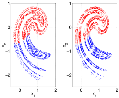
Figure 1: Left: partition estimated by SFNN optimization on 2000 data points from the Ikeda map. Right: partition calculated with foreknowledge of UPOs, numerically extracted from the equation of motion. The partition we estimate from observed data alone is quite close to a presumably correct one, calculated from the method of davidchack . The measure on the two figures is not the same: the left figure is a sample of the natural measure, whereas the right shows UPOs up to period 16. They avoid regions of homoclinic tangencies, contributing to the blank spaces.

For concrete numerical calculations, we need to parameterize partitions with a relatively small number of free parameters. Inspired by davidchack , we define partitions with respect to a set of radial-basis “influence” functions of the form $f_{k}({\bf x})=\alpha_{k}/||{\bf x}-{\bf z}_{k}||^{2}$, the set of $\alpha$ and ${\bf z}$ being the free variables. For any particular ${\bf x}$, one $f_{l}({\bf x})$ will generically result in the largest value versus other $f_{k}({\bf x}),k\neq l$, and then ${\bf x}$ is assigned to that symbol which was pre-assigned to influence function $f_{l}$. The ${\bf z}$ parameters are initialized to random examples from the ${\bf x}_{i}$ and $\alpha$ to independent random variates $[0,1)$, and $n_{f}$ functions assigned to each of the $A$ symbols. In davidchack the ${\bf z}_{k}$ were fixed on the UPOs and their symbols varied; here, the centers and coefficients vary but their symbols are fixed. We minimize $J_{\text{sfnn}}$ or $K_{\text{sfnn}}$ over the $An_{f}(d+1)$ free parameters using “differential evolution” diffevol , a genetic algorithm suitable for continuous parameter spaces.

Figure 1 shows the final ${\cal P}$ on 2000 data points from the Ikeda mapikedamap . It shows the best result (lowest $J_{\text{sfnn}}$) out of six restarts changing only the random seed governing the initial conditions; the results were not much worse on the other runs, however. The result is very close to the partition knowing the dynamics.

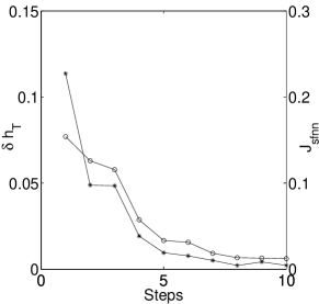
Figure 2: For each new best partition: Minimization target $J_{\text{sfnn}}$ (circles, and right scale), estimated deficiency in topological entropy ${\delta h}_{T}$ (asterisks and left scale) Minimizing $J_{\text{sfnn}}$ generally minimizes ${\delta h}_{T}$ and thus maximizes topological entropy of the symbolic language.

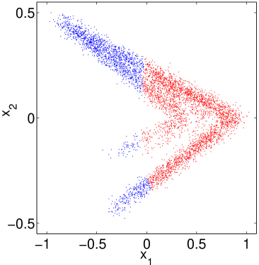
Figure 3: Minimizing $K_{\text{sfnn}}$ with $\gamma=0.01$: estimated partition for a time series of 5000 data points from the Lozi map with 10% additive by amplitude Gaussian noise. Either the $x_{1}$ or $x_{2}$ axes are GPs for the noiseless map. Here despite the noise the algorithm finds a partition close to what would be a GP.

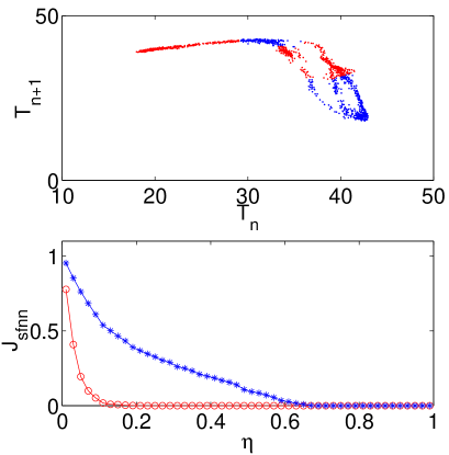
Figure 4: Top: estimated binary partition for time-delay embedding of inter-bubble time intervals (arbitrary units), minimizing $K_{\text{sfnn}}$. Bottom: $J_{\text{sfnn}}(\eta)$ vs $\eta$ for the optimized partition (circles) and for a naive equiprobable histogram partition with the same alphabet (asterisks). For the optimized partition there are very few large distance errors, e.g. $J_{\text{sfnn}}$ observed above $\eta=0.1$.

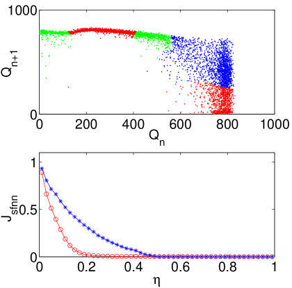
Figure 5: Same as Fig. 4 but with combustion engine heat release time series (energy, arbitrary units), and $A=3$. The noise level is higher thus there remain more moderately sized distances, even with a larger alphabet which usually results in better localization.

In a stationary information source, the number of distinct length-$p$ codewords will scale, for asymptotic $p$, as $N_{p}\propto e^{h_{T}p}$ where $h_{T}$ is the topological entropy, a dynamical invariant. We validate ${\cal P}$ with an estimate of the deficiency between $h_{T}$ implied by ${\cal P}$ and the correct $h_{T}$: ${\delta h}_{T}={p_{\text{max}}}^{-1}\sum_{p=1}^{p_{\text{max}}}{p}^{-1}\log\left(N_{p}/\tilde{N}_{p}\right)$. $N_{p}$ is the number of distinct period-$p$ UPOs (which were computed knowing the equations of motion), $\tilde{N}_{p}$ the number of such UPOs with unique $p$-symbol codes in some ${\cal P}$. A GP gives ${\delta h}_{T}=0$, and ${\delta h}_{T}\rightarrow 0$ for better (less UPO-degenerate) partitions. Figure 2 shows ${\delta h}_{T}$ on each new best partition found during the optimization. The optimization target, $J_{\text{sfnn}}$, decreases strictly monotonically by construction; though ${\delta h}_{T}$ does not decrease quite monotonically, the trend toward very small values is clear. This gives evidence that minimizing $J_{\text{sfnn}}$ also refines approximations to GPs.

Figures 3–5 demonstrate applications of the algorithm. Fig. 3 shows the effect of noise on a system where the GP is analytically known. The Lozi map (see analysis in henonsymbols ) is similar to the Henon map but replaces the quadratic nonlinearity with a piecewise linear one. We find a partition which is close to the noise-free GP even when the data have been contaminated by significant amounts of additive noise. Though complete localization to a single point is not possible here, minimizing large divergences is still a desirable criterion. Figures 4 to 5 show estimated partitions on experimental data sets where no analytical form of the equations (much less partitions) are known. On account of noise, dynamical or observational, a certain amount of divergence $D$ for symbolic nearest neighbors is inevitable. Still, minimizing large deviations is a reasonable goal even for noisy data. There are very few rank distances with $R\geq 0.2$ or $0.3$ compared to a basic histogram partition.

It must be kept in mind that GPs are not necessarily unique for any attractor. Distinctly different partitions may be found, all of which are reasonably satisfactory. (At a minimum any iterate of a GP is also a GP). There are many coexisting solutions (roughly like finding low-energy states of a spin glass), which is why the optimization problem is hard, requiring a global search method. We conjecture this is one reason why understanding the structure of generating partitions has been so difficult for mathematicians.

We also point out that it is possible to partition one space ${\bf x}$, but quantify distances $D_{i}=||{\bf z}_{{\cal N}[i]}-{\bf z}_{i}||$ in some different space as long as there is some relation between each ${\bf x}_{i}$ and ${\bf z}_{i}$. For example, one may be interested in a simple symbolic control scheme, say where ${\bf z}_{i}={\bf x}_{i+T}$ (find the best partition of observables now that best predicts some future), or perhaps when two different variables are measured simultaneously and one wants to cross-predict. In the first case, in principle, a GP should be optimal for predicting the future as well as the present but the inevitable issues of finite data and noise may make the best empirical partition different for the two cases. In the second case, generating partitions are irrelevant entirely.

References

- (1) Among many others in the literature, P. Graben., J. D. Saddy, M. Schlesewsky, J. Kurths, Phys. Rev. E 62 5518–5541 (2001), M. Lehrman, A. B. Rechester, Phys. Rev. Lett. 87 164501-1ff (2001), Z. Hongxuan, Z. Yisheng, Medical Engr. & Phys 23 523–528 (2001), J. Godelle, C. Letellier, Phys. Rev. E, 62 7973–7981 (2000), R. Steuer, W. Ebeling, D. F. Russell, S. Bahar, A. Neiman, F. Moss, Phys. Rev. E, 64 061911-(1-6) (2001). An applied review is, C. S. Daw, C. E. A. Finney, E. R. Tracy, “Symbolic analysis of experimental data”, http://www-chaos.engr.utk.edu/pap/crg-rsi2002.pdf.
- (2) We assume that an appropriate state space of sufficient dimension has been constructed from the observed data, and dynamics on it are as a discrete map—for flows a Poincare section is taken. The methods in M. B. Kennel, H. D. I. Abarbanel, Phys. Rev. E, 66 026209 (2002). M. B. Kennel, R. Brown, H. D. I. Abarbanel, Phys. Rev. A, 45 3403–3411 (1992), among others, may be helpful for validating a good embedding. The present partition method cannot correct for an improper embedding of the continuous space.
- (3) E. M. Bollt, T. Stanford, Y-C. Lai, K. Zyczowski, Physica D, 154 259–286 (2001).
- (4) R. L. Davidchack, Y-C. Lai, E. M. Bollt, M. Dhamala, Phys. Rev E 61 1353–1356 (2000)
- (5) R. Steuer, L. Molgedey, W. Ebeling, M. A. Jimenez-Montano, Eur. Phys. J. B, 19 265–269 (2001)
- (6) P. Cvitanovic, G. H. Gunaratne, I. Procaccia, Phys. Rev. A, 38 1503- (1988).
- (7) Y-C Lai, E. Bollt, C Grebogi, Phys. Lett A 255 75–81 (1999)
- (8) J. H. Friedman, J. L. Bentley , and R. A. Finkel ACM Trans. Math. Software 3, 209–226, (1977). R. F. Sproull, Algorithmica 6, 579–589 (1991).
- (9) M. B. Kennel, H. D. I. Abarbanel, Phys. Rev. E, 66 026209 (2002). M. B. Kennel, R. Brown, H. D. I. Abarbanel, Phys. Rev. A, 45 3403–3411 (1992)
- (10) R. Storn, K. Price, Jour. Global Optimization, 11 341–359 (1997).
- (11) Dynamical equations and parameters are as in davidchack .
- (12) K. Nguyen, C. S. Daw, P. Chakka, M. Cheng, D. D. Bruns, C.E.A. Finney, M. B. Kennel, Chemical Engineering Journal 64(1): 191-197, (1996)
- (13) R. M. Wagner, J. A. Drallmeir, C. S. Daw, Int. J. Engine Research, 1 301–320 (2000)