Generalized dynamical entropies in weakly chaotic systems

Abstract

A large class of technically non-chaotic systems, involving scatterings of light particles by flat surfaces with sharp boundaries, is nonetheless characterized by complex random looking motion in phase space. For these systems one may define a generalized, Tsallis type dynamical entropy that increases linearly with time. It characterizes a maximal gain of information about the system that increases as a power of time. However, this entropy cannot be chosen independently from the choice of coarse graining lengths and it assigns positive dynamical entropies also to fully integrable systems. By considering these dependencies in detail one usually will be able to distinguish weakly chaotic from fully integrable systems.

1 Introduction

Dynamical entropies measure rates at which information may be gained by observing a system of interest subjected to some law of temporal evolution. For deterministic dynamics one considers the time evolution of an initial ensemble of systems distributed uniformly inside a small compact box of diameter $\epsilon$ (typically a ball or a cube) within the phase space characterizing the possible states of the system. One then asks how many boxes of size $\epsilon$ are at least needed to cover the image of the initial box after a time $t$ has elapsed. If, in the limit $\epsilon\to 0$, the natural logarithm of this number increases as $h_{top}t$ asymptotically for $t\to\infty$, the quantity $h_{top}$ is called the topological entropy. In physical applications usually the Kolmogorov-Sinai entropy, designated as $h_{KS}$ is more relevant. This is defined in similar way, but the covering set is not required to contain the full image of the initial box; it only has to cover this up to a subset of measure $\mu(t)$ satisfying $\lim_{t\to\infty}\mu(t)=0$. To interpret this, assume $\epsilon$ is the minimal resolution with which one may distinguish phase space points by physical observation. Then by repeating the observations at regular time intervals the number of distinguishable initial boxes increases as $\exp h_{KS}t$ for a typical large but not exhaustive number of observed systems and it increases as $\exp h_{top}t$ for an exhaustive search in which also rare events are weighted properly for the full time range of observation.

For chaotic dynamical systems that are closed (no points escape from phase space) Pesin’s theorem equates the KS-entropy to the sum of the positive Lyapunov exponents. Intuitively this result is not hard to understand. Each positive Lyapunov exponent $\lambda_{i}$ corresponds to an independent direction in phase space with a smooth expansion by a factor of roughly $\exp\lambda_{i}t$ over a time $t$. So the overall expansion factor, and thereby the number of boxes needed to cover the image of the initial box, increases as $\exp\sum_{i}\lambda_{i}t$. A priori one could expect though, that, at least in part, this may be offset by shrinkage in the contracting directions. However, this contraction typically takes place towards a fractal set with a striated structure on increasingly finer length scales. Once the typical length scale of separation between striation sheets falls below the box size $\epsilon$ the number of boxes required to cover the set does not decrease any more. For comparison: consider the number of intervals of length $\epsilon$ needed to cover successive approximations of the middle-third Cantor set. Once the length of the subintervals that are erased at the next iteration falls below $\epsilon$ the number of covering intervals essentially does not change any more. The difference between topological and KS-entropy may be understood again by observing that on subsets of phase space of measure zero the Lyapunov exponents may differ from the ”bulk” Lyapunov exponents, which for an ergodic system are constant almost everywhere.

There exist dynamical systems that are not chaotic, in the ususal sense of having at least one positive Lyapunov exponent, but still show a fairly rapid decay to equilibrium, related to motion in phase space that appears very random. Simple examples of these are wind tree models, in which light particles without any mutual interaction move elastically among fixed polygonal scatterers. Lepri et al.[1] numerically studied such a model consisting of diamond shaped scatterers with corner angles that are irrational fractions of $\pi$ on a triangular lattice with bounded free paths between collisions. They found this model equilibrates rapidly on the projection to the unit cell in space times the unit sphere for the velocities, and on large time and length scales it is described by normal diffusion. Dettmann et al.[3] looked at Ehrenfests original wind tree model[2], in which the scatterers are randomly distributed parallel squares and the velocities of the light particles always point along the diagonals of the squares. In this case the velocities equilibrate among the four allowed directions and, in finite volume the density of a cloud of light particles becomes uniform. Again, on large time and length scales the dynamics becomes diffusive, provided the scatterers are not allowed to overlap each other[4, 5, 6]. Another variation, studied by Li et al.[7], consists of a channel lined by triangular scatterers, through which light particles move, giving rise again to diffusive motion on large scales. Other non-chaotic systems leading to macroscopically stochastic looking motion are mixtures of point particles of different masses in one dimension. These, for $N$ particles, may be viewed as a type of wind tree model on a $2N$-dimensional phase space bounded by flat hyperplanes. The intersections between these hyperplanes take the role of the corners; ”hitting the other side of a corner” translates to an interchange in the sequence of two subsequent collisions. Livi et al.[8] and Grassberger et al.[9] found that such systems show anomalous hydrodynamics, which is typical for one-dimensional systems. As a last example I would like to mention systems of many moving parallel oriented polygons (in 2d) or polyhedra (in 3d), which in collisions exchange the velocity components normal to the plane of collision. These systems too may be viewed as wind tree like models in a high dimensional phase space. No doubt they will show normal hydrodynamics (up to the usual nonlinearities in 2d, see e.g. [10]) although they are obviously non-chaotic. But to my knowledge no detailed investigations have been done for such systems so far.

For the systems described above, according to Pesin’s theorem the KS-entropy equals zero. Yet, it is clear that information may be gained by repeated observation, only the number of distinguishable initial boxes will not increase exponentially with time, but rather as a power law. Zaslavsky and Edelman refer to this situation as pseudochaos[11]. I will use the term ”weak chaos” in the sequel, without giving a precise definition. For quantifying the power law increase of the information on the initial distribution Tsallis’ formalism seems suitable, as it is precisely meant to define an entropy for systems in which the countable number of states (here distinguishable initial boxes) does not increase exponentially with system size (here time) but rather as a power law. But there are some subtleties here to deal with. As we will see, the dynamical entropy as defined usually, will become dependent on the coarse graining lengths in the system. It has to be multiplied by powers of these to allow for taking the limit $\epsilon\to 0$. In addition, even very regular systems, such as an ideal gas in a periodic box, or a weakly anharmonic oscillator, will turn out to give rise to a positive dynamic Tsallis entropy, thereby excluding this property by itself as an indicator of weak chaos. Keeping track of the power law by which the information increases may help to recognize weak chaos. Even this requires a lot of care, because the powers of time resulting from integrable degrees of freedom may vary, depending on the type of motion they represent.

In the next sections we will consider dynamical Tsallis entropies and look at wind tree models in detail. In the discussion the feasibility of using a dynamical Tsallis entropy to characterize weak chaos will be discussed further.

2 Dynamical Tsallis entropies

Supose the phase space of a class of dynamical systems is divided into subsets $C_{i}$ such that the probability of finding a system in $C_{i}$ equals $p_{i}$. Then the Tsallis entropies are defined through.

$$S_{q}=\frac{1-\sum_{i}p_{i}^{q}}{q-1.}$$ (1)

Here $q$ is a free parameter the choice of which should be dictated by the properties of the system considered. In the limit $q\to 1$ the Tsallis entropy reduces to the usual entropy.

In the case of dynamical systems evolving in time from the interior of an initial set of diameter $\epsilon$ one may choose for the $C_{i}$ a covering set of non-intersecting subsets of diameter $\epsilon$ and define $p_{i}(t)$ as the fraction of initial phase points that end up inside $C_{i}$ after the time evolution over time $t$. The number of $C_{i}$ with non-vanishing $p_{i}(t)$ will increase as a power of $t$. Now let us suppose that on this subset $p_{i}(t)$ for large $t$ behaves as

$$p_{i}(t)=\frac{w_{i}}{Ct^{\alpha}},$$ (2)

with $w_{i}$ distributed according to some probability distribution with a mean value of unity. Then, in order for $S_{q}(t)$ to increase proportionally to $t$ one has to choose $q=1-1/\alpha$. In this case the entropy behaves as

$$S_{1-1/\alpha}(t)=\alpha C^{1/\alpha}<w_{i}^{(1-1/\alpha)}>,$$ (3)

with the brackets indicating an average over the distribution of $w_{i}$. In case this is an exponential distribution, $p(w)=\exp-w$, one finds $<w_{i}^{(1-1/\alpha)}>=\Gamma(2-1/\alpha)$.

A further remark is required here. As time increases one should choose increasingly smaller values of $\epsilon$ in order to avoid $C_{i}$’s containing parts of the image of several initial boxes. For fixed $\epsilon$ this will always occur after sufficiently long time. In principle one should take a limit $\epsilon\to 0$ followed by the limit $t\to\infty$. We will see however that the generalized dynamical entropies one would like to define are dependent on $\epsilon$, so one cannot take these limits in a straightforward way. In fact, as we will see, it can only be done after redefining the dynamical entropies in an appropriate way.

3 Wind tree models

Here I will consider a wind tree model in two dimensions with square scatterers of side length $a$ that are randomly oriented and distributed randomly over a rectangle with periodic boundary conditions.

Figure 1: A configuration of the wind tree model with randomly oriented square scatterers. The dashed line represents a posible light-particle trajectory (note the periodic boundary conditions)

The scatterers are not allowed to overlap each other. I will assume that the density $\rho$ of scatterers is small, that is $\rho a^{2}\ll 1$, so subsequent collisions of a light particle are to a very good approximation uncorrelated. For the subsets $C_{i}$ of the phase space let us choose small rectangular blocks of side lengths $\epsilon_{r}$ in position space and $\epsilon_{v}$ in velocity space. Over a time $t$ the dynamics stretches out these blocks into parallellopipida. For large $t$, in the direction parallel to the velocity these obtain an extension of length $\epsilon_{v}t$. In the direction orthogonal to the velocity the front width covered by the parallellopipidum also grows as $\epsilon_{v}t$. In addition the block is split into two subblocks, as illustrated in Fig. 2, as soon as its front hits a corner of one of the scatterers.

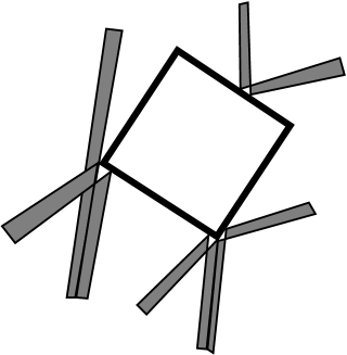
Figure 2: When a block of nonzero density in phase space hits a corner of a scatterer it is split into two subblocks. If it just hits a side it is reflected in its entirety.

Next, when one of the two subblocks hits another corner it is split up likewise and so on. The total front width of all the propagating subblocks increases with time as $\epsilon_{v}t$, independent of the number of splittings that have taken place. Therefore the average number of splittings during a long time $t$ is given by

$$N(t)=\frac{3}{2}\rho v\epsilon_{v}t^{2}.$$ (4)

Here $v$ is the average speed of a light particle. The average area swept out by the total front of all the subblocks is $v\epsilon_{v}t^{2}/2$ and this is multiplied by $3\rho$ to obtain the average number of visible corners in this area. The average number of resulting subblocks is almost equal to $N(t)$. To obtain the number of subsets $C(i)$ needed to cover all of the subblocks at $t$ one has to multiply $N(t)$ by $\epsilon_{v}t/\epsilon_{r}$, the number of subsets needed to cover the extension in the parallel direction. So in Eq. (2) $\alpha=3$ and $C=3\rho v\epsilon_{v}^{2}/2\epsilon_{r}$. The positions of the corners with which the collisions take place follow a Poisson distribution along the front, hence the distribution of $w_{i}$ is an exponential one indeed. Using the results of the preceding section we find

$$S_{2/3}(t)=\alpha t\left(\frac{3\rho v\epsilon_{v}^{2}}{2\epsilon_{r}}\right)^{2/3}\,\Gamma\left(\frac{5}{3}\right).$$ (5)

4 Discussion

The first thing that draws the attention in Eq. (5) is the dependence of the entropy on the coarse graining lengths $\epsilon_{v}$ and $\epsilon_{r}$. This is a striking difference from the result found by Borges et al.[12] for the logistic map at the onset of chaos. Here too the number of boxes increases algebraically with time, but this is due to a power law separation between infinitesimally close trajectories in phase space. In the wind tree models infinitesimally close trajectories typically just separate linearly with time, due to the infinitesimal velocity difference, but the interesting power law behavior in the time dependence of the number of covering sets needed is caused by the corner induced splitting of trajectories at arbitrarily small, but always finite distances from each other. The same is true for all the other examples mentioned in the introduction. As mentioned at the end Sec. 2 a sharp definition of dynamical entropies involves taking a limit $\epsilon\to 0$ followed by the limit $t\to\infty$. Obviously this makes no sense for the entropy obtained in Eq. (5). The limit $\epsilon\to 0$ is not well-defined. Apparently the only way to repair this is by defining still another dynamical entropy as

$$\tilde{S}_{q}=\left(\frac{\epsilon_{r}}{\epsilon_{v}^{2}}\right)^{q}S_{q}.$$ (6)

An alternative way of obtaining this is by requiring $\epsilon_{r}=\epsilon_{v}^{2}$. For wind tree like models in $d$ dimensions the prefactor $\epsilon_{r}/\epsilon_{v}^{2}$ should be raised to the power $d-1$. This solution is not very elegant, e.g. there seems to be no obvious choice for making the $\epsilon$’s dimensionless. But at least it seems to give a proper limiting behavior for $\epsilon\to 0$ for all wind tree like models.

A second point of concern is the entropy of an ideal gas in a periodic box. One easily sees that, with the same type of covering sets as for the wind tree model, the number of sets needed to cover the time evolved initial set increases in $d$ dimensions as $(\epsilon_{v}t/\epsilon_{r})^{d}$. So for $q=1-1/d$ one now has a dynamical entropy that increases linearly with time. The same occurs for other integrable systems in which the periods of the angle variables depend on the values of the action variables. This is usually the case, with harmonic oscillators being the notable exception. For $d$-dimensional wind tree models the power of $t$ by which the number of needed covering sets increases with time is $2d-1$. So it looks like one could use the condition $q>1-1/d$ as a criterion for weak chaos in a $d$-dimensional hamiltonian system. Here too care is needed. For example in a three-dimensional system that is a wind tree model in the $x-y$ plane but in addition performs a harmonic oscillation in the $z$-direction, one has $q=1/3$, just as for a three-dimensional ideal gas. A distinction between the two cases may still be found in the dependence of $S_{2/3}$ on $\epsilon_{r}$ and $\epsilon_{v}$. The powers of $\epsilon_{v}$ and $\epsilon_{r}$ by which one has to multiply $S_{q}$ in order to obtain a $\tilde{S}$ with a proper limit for $\epsilon\to 0$ obviously are different for integrable systems of various types, for wind tree like models and for mixed systems.

It is not hard constructing generalizations of the wind tree model to higher dimensions. One just has to replace the scatterers by polyhedra of appropriate dimension. And indeed for each direction orthogonal to the velocity one picks up a factor $t^{2}$ in the growth factor of $N(t)$. Similar observations can be made for the moving polygons.

To conclude: Dynamical Tsallis entropies may be useful for characterizing weakly chaotic systems in which the information on initial conditions increases as a power law rather than an exponential. For wind tree like systems however, the precise value of this entropy depends on the choice of the coarse-graining lengths, which basically sets the smallest scales on which one may distinguish different systems in a single observation. To obtain a dynamical entropy with a proper limit when these coarse graining lengths are sent to zero, one first has to multiply the ”straightforward” dynamical entropy with appropriate powers of the coarse graining lengths. Further, the generalized entropies typically assume non-zero values also for integrable systems. In many cases the $q$-values needed to find an entropy that increases linearly with time will allow one to distinguish wind tree like systems from integrable ones, but this too is not always the case. If not, the dependence on the coarse graining lengths may be used for a further distinction.

HvB acknowledges support by the Mathematical physics program of FOM and NWO/GBE.

References

- [1] S. Lepri, L. Rondoni and G. Benettin, J. Stat. Phys. 99 (2000) 857
- [2] P. Ehrenfest, Collected scientific papers (North Holland, Amsterdam 1959)
- [3] C. P. Dettmann, E. G. D. Cohen and H. van Beijeren, Nature 401 (1999) 875; C. P. Dettmann and E. G. D. Cohen, J. Stat. Phys. 103 (2001) 589
- [4] E. H. Hauge and E. G. D. Cohen, J. Math. Phys. 10 (1969) 397
- [5] W. W. Wood and F. Lado, J. Comp. Phys. 7 (1971) 528
- [6] H. van Beijeren and E. H. Hauge, Phys. Lett. 39A (1972) 397
- [7] B. Li, L. Wang and B. Hu, Phys. Rev. Lett. 88 (2002) 223901
- [8] R. Livi, A. Politi and S. Ruffo, J. Phys. A: Math. Gen. 19 (1986) 2033
- [9] P. Grassberger, W. Nadler and L. Yang, Phys. Rev. Lett. 89 (2002) 180601
- [10] M. A. van der Hoef and D. Frenkel, Phys. Rev. A 41 (1990) 4277
- [11] G. M. Zaslavsky and M. Edelman, nlin.CD/0112033
- [12] E. P. Borges, C. Tsallis, G. F. J. Añaños and P. M. de Oliveira, Phys. Rev. Lett. 89 (2002) 254103