Current address: ]School of Mathematics and Statistics, University of New South Wales at ADFA 2600, ACT, Australia

Light bullets in quadratic media with normal dispersion at the second harmonic

Abstract

Stable two- and three-dimensional spatiotemporal solitons (STSs) in second-harmonic-generating media are found in the case of normal dispersion at the second harmonic (SH). This result, surprising from the theoretical viewpoint, opens a way for experimental realization of STSs. An analytical estimate for the existence of STSs is derived, and full results, including a complete stability diagram, are obtained in a numerical form. STSs withstand not only the normal SH dispersion, but also finite walk-off between the harmonics, and readily self-trap from a Gaussian pulse launched at the fundamental frequency.

A multidimensional soliton is a self-supporting solitary pulse resulting from the balance between nonlinearity of the medium and diffraction and dispersion of the wave field. The most physically relevant realization of this is provided by optical spatiotemporal solitons (STSs), alias “light bullets”, which are self-confined in the longitudinal and transverse directions Yaron .

Spatial optical solitons, which are not localized in the longitudinal direction, have been studied in depth review , and observed in both one- 1d and two- 2d dimensional (1D and 2D) geometries. Quasi-2D STSs, which are localized in the longitudinal and one transverse directions, have been observed too Liu99 . A challenge for the experimentalist is creating a fully 3D bullet. The issue has a special physical purport, as, unlike 2D solitons which occur in various media, optical crystals provide for a single real possibility to create 3D solitons in classical physics. Besides their significance as fundamental objects, STSs may provide THz switching rates in optic-logic systems, if used as information bits Macleod .

It is well known that STSs are unstable in Kerr media Rasmussen . They can be stabilized if the nonlinearity is saturable Blagoeva . Other effects can also stabilize a spatiotemporal pulse, as shown in an experiment demonstrating stable space-time focusing in a planar waveguide Eisenberg . However, it was not a soliton, as the stabilization was due to multi-photon absorption and intra-pulse Raman scattering, which are dissipative effects.

A promising path for making stable STSs is to employ second-harmonic generation (SHG). Various types of solitons in SHG materials have attracted a lot of interest Buryak . In particular, it was proven long ago Kanashov , by means of variational estimates, that SHG must give rise to stable 2D and 3D solitons realizing a minimum of the Hamiltonian.

Most theoretical works on STSs in SHG media assumed spatiotemporal isotropy Skr , which implies equal GVD (group-velocity-dispersion) coefficients at the fundamental frequency (FF) and second harmonic (SH), that does not take place in reality. A general non-symmetric case was considered in Ref. Malomed97 . Using the variational approximation (VA), STSs were predicted, and numerical simulations verified their stable existence in the 2D case. Later, numerically exact 2D and 3D soliton solutions were found and their stability was confirmed Mihalache98 . Then, another ingredient important for the description of the real physical situation was introduced, namely, the group-velocity mismatch (GVM, alias walkoff) between the harmonics, showing that stable STSs exist in this case too Mihalache99a .

It is obvious that solitons in SHG media may only exist if GVD is anomalous at FF. Even without postulating the above-mentioned spatiotemporal isotropy, all the previous works assumed that GVD must be anomalous at SH too. However, this assumption ignores a fundamental problem: in available SHG materials, FF suffers strong absorption if the SH wavelength is long enough for the dispersion to be anomalous. Note that, in Ref. Malomed97 , VA formally predicted STSs for normal GVD at SH, but simulations led to conclusion that it could really exist only with anomalous GVD at SH, while the prediction for the normal SH dispersion was an artifact of VA based on the Gaussian ansatz, which incorrectly treats exponentially decaying tails of the soliton (see a discussion of the role of the tails below). In the 3D case, VA predicted that STSs could exist at small normal values of GVD at SH, but this was never checked. Besides its crucial importance for the creation of LBs in experiment, the issue is also a challenge for analysis of multidimensional nonlinear-wave models.

In this work we demonstrate that, contrary to the common belief, STSs in the 3D and 2D cases effectively exists and can be stable in SHG media with normal GVD at SH. We also conclude that it survives in the presence of GVM. These results greatly enhance the likelihood that STSs will be generated experimentally.

The co-propagation of the FF and SH waves in SHG media is described by known equations Kanashov ; Malomed97 ,

$$iu_{\xi}+\nabla_{\bot}^{2}u+u_{\tau\tau}-u+u^{\ast}v = 0,$$ (1)

$$2iv_{\xi}+\nabla_{\bot}^{2}v+\delta v_{\tau\tau}-i\sigma v_{\tau}-\gamma v+\left(1/2\right)u^{2} = 0.$$ (2)

Here, $u=\sqrt{2}\mathcal{E}_{1}e^{-iz/z_{0}}z_{0}\omega_{1}^{2}\chi^{(2)}/(k_{1}c^{2})$ and $v=\mathcal{E}_{2}e^{-2iz/z_{0}}z_{0}\omega_{1}^{2}\chi^{(2)}/(k_{1}c^{2})$, $\mathcal{E}_{1,2}$ are complex electric-field envelopes at the frequencies $\omega_{1}$ and $2\omega_{1}$, $k_{1}\equiv k\left(\omega_{1}\right)$ is the FF carrier wavenumber, $\xi=z/z_{0}$ and $\tau=(t-z/v_{g})/t_{0}$ are the normalized propagation distance and reduced time, $v_{g}$ and $t_{0}$ being the group velocity and time scale at FF, $z_{0}=2t_{0}^{2}/k_{1}^{{}^{\prime\prime}}$, where $k_{1}^{{}^{\prime\prime}}$ is the GVD coefficient at FF, and the transverse radial coordinate is $r=\sqrt{2k_{1}\left(x^{2}+y^{2}\right)/z_{0}}$. The diffraction operator, $\nabla_{\bot}^{2}\equiv\partial^{2}/\partial r^{2}+[(D-2)/r]\partial/\partial r$, where $D=3$ or $2$ is the spatial dimension, acts on the transverse coordinates $\{x,y\}\equiv\sqrt{2k_{1}/z_{0}}\mathbf{r}$. In the experiment, units of time and transverse and propagation distance in the scaled equations typically correspond to $100$ fs, $50$ $\mu$m, and $1$ cm, respectively Liu99 . Further, $\sigma$ in Eq. (2) is GVM, and $\gamma\equiv 4+2z_{0}[2k(\omega_{1})-k(2\omega_{1})]$ is the phase mismatch between the harmonics. The equations conserve the Hamiltonian, momentum, axial angular momentum, and the Manley-Rowe invariant (energy), which is $Q=2\pi\int_{0}^{\infty}rdr\int_{-\infty}^{+\infty}d\tau\,\left(|u|^{2}+4|v|^{2}\right)$ in the 3D case.

In Eq. (1), the FH dispersion is anomalous, while the ratio $k_{2}^{{}^{\prime\prime}}/k_{1}^{{}^{\prime\prime}}\equiv\delta$ of the SH and FH GVD coefficients is assumed negative, corresponding to normal GVD at SH. This case, which corresponds to the experimental reality, has not yet been studied (except for VA, with $\sigma=0$, in Ref. Malomed97 ).

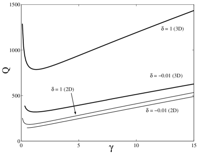
Figure 1: The energy of stationary spatiotemporal solitons vs. the phase mismatch $\gamma$ in the case of normal GVD at the second harmonic ($\delta=-0.01$). The curves with $\delta=1$ represent earlier known solutions and are included for comparison.

First, an estimate for the existence of STSs can be obtained for small $|\delta|$. To this end, Eq. (2) is treated as a linear equation for SH, driven by the term $\left(1/2\right)u^{2}$. A SH field component of the CW (continuous-wave) form, $B_{\mathrm{cw}}\exp\left(i\mathbf{k\cdot r}-i\omega\tau\right)$, which does not vanish as $r,|\tau|\rightarrow\infty$ and thus prevents the existence of the soliton, is determined by zeros of the denominator of the corresponding Green’s function, which are located at

$$|\delta|\omega^{2}-\sigma\omega-k^{2}-\gamma=0.$$ (3)

On the other hand, an asymptotic form of the solution to Eq. (1) at $r,|\tau|\rightarrow\infty$ is $u\sim\rho^{-(D-1)/2}\exp\left(-\rho\right)$, with $\rho\equiv\sqrt{\tau^{2}+r^{2}}$.

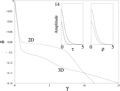
Figure 2: Stability regions for 2D and 3D solitons without walkoff ($\sigma=0$). The solitons are stable above the respective borders. The insets show central profiles of the 3D soliton in the temporal and spatial directions, for $\delta=-0.02$ and $\gamma=5$. The upper and lower curves pertain to the FF and SH components $u$ and $v$, respectively.

An estimate for the maximum amplitude $B_{\mathrm{cw}}$ of the possible CW component can be derived. To simplify the presentation, one can adopt a model form of the FF field complying with the above asymptotics and securing a globally correct shape of the solution. In the 3D case, it is $u=\mathrm{const\cdot}\rho^{-1}\left(\sinh\rho\right)\mathrm{sech}^{2}\rho$, but the final exponential estimate (see below) does not predicate on this “ansatz”. Straightforward calculations [Fourier transform of $u^{2}(\mathbf{r},\tau)$, inverse transform of its product with the Green’s function of Eq. (2), and isolating a CW contribution from $\omega$ determined by Eq. (3)] show that, in the case $\sigma=0$ (no-walkoff), the CW intensity is exponentially small (for small $|\delta|$) if $\gamma>0$, an upper estimate for it being

$$B_{\mathrm{cw}}^{2}<\mathrm{const}\cdot\gamma\left(\gamma/|\delta|\right)^{3/2}\exp\left(-\pi\sqrt{\gamma/|\delta|}\right).$$ (4)

While the pre-exponential part of this estimate may be ansatz-dependent, the crucially important exponential part is not, and it applies to the 2D case as well; if $\sigma\neq 0$, it is replaced by $\exp\left\{-\pi\left[\sqrt{\left(\gamma/|\delta|\right)+\left(\sigma/2\delta\right)^{2}}-\left|\sigma/2\delta\right|\right]\right\}$, i.e., the walkoff makes the estimate weaker.

Thus, although it is not guaranteed that the STS exists as a rigorous solitary-wave solution, the one with the CW tail obeying the exponentially small estimate may be tantamount to a true soliton in any possible experiment. The actual region of the existence and stability of STSs should be found numerically, which is done below.

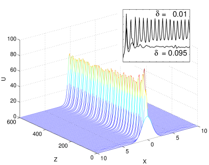
Figure 3: Evolution of the 3D soliton self-trapping from an initial Gaussian pulse for $\delta=-0.01,\gamma=1$, and $\sigma=0$. The propagation distance corresponds to $\approx 800$ dispersion lengths. The inset shows the evolution of the FF amplitude on a shorter scale, for the same case and the one with $\delta=0.095$, closer to the instability border.

Stationary solutions were found by solving the $z$-independent version of Eqs. (1) and (2) with $\delta<0$. Although the above analysis suggests that STS may have a small nonvanishing tail in the SH component, no tails were found, with the numerical accuracy available [$\mathcal{O}(10^{-4})$], in all the pulses which were identified as solitons. It was also verified that the shape of the soliton does not change with increasing the numerical accuracy and/or size of the integration domain (for instance, there was no change with the increase of the number of points from $64^{3}$ to $256^{3}$). Insets in Fig. 2 show an example of a 3D soliton, found for $\delta=-0.02$, $\gamma=5$ and $\sigma=0$. An STS family was generated by varying $\delta$ and $\gamma$, Fig. 1 showing the soliton’s energy versus $\gamma$. A conclusion of direct relevance to experiment is that, in the most challenging 3D case, energy required to create a soliton with normal GVD at SH is smaller than in the previously studied case $\delta=1$ by a factor $\simeq 2.5$.

Further consideration shows that, at large $\gamma$, the bulk of the STS’s energy is in FF (in compliance with the cascading limit Buryak ), while at smaller $\gamma$ the amplitudes of both components are nearly equal, hence SH has roughly four times the energy of the fundamental. This shows that, remarkably, the soliton is able to exist keeping $\simeq 80\%$ of its energy in the normal-GVD component.

A crucially important issue is stability of the solitons. First of all, it may be judged using the Vakhitov-Kolokolov criterion, which states that solitons may only be stable if $dQ/d\gamma>0$ Buryak . Figure 1 shows that the soliton families satisfy this criterion, unless $\gamma$ is too small. A systematic stability test was performed by direct simulations of Eqs. (1) and (2). The results are summarized in Fig. 2.

At small $|\delta|$, the stability border in Fig. 2 is linear, which complies with the fact that the exponential factor in the estimate (4) is a function of the ratio $\gamma/|\delta|$ (the exponential estimate yields a factor $\sim 10^{-5}$ at the stability border in the figure). Furthermore, the 2D and 3D stability borders are almost identical at small $|\delta|$, in agreement with the fact that the exponential estimate is the same for both dimensions. The solitons are truly robust: not only they are not destroyed by perturbations, but they also readily self-trap from initial pulses of quite an arbitrary shape, which is illustrated by Fig. 3. Note that the transition from the initial profile to the soliton’s one takes the propagation distance of few dispersion lengths ($z_{D}$), and the STS remains stable over an extremely long distance $\approx 800z_{D}$. This shows not only that the STS will be stable in any experimental setup, but also that possible energy leakage due to the formation of the above-mentioned CW tail cannot be spotted in the course of the extremely long propagation. The same figure shows persistent intrinsic oscillations in the stable STS, which is attributed to excitation of an intrinsic mode. The excitation is tangible if the initial pulse is launched at a point which is located deep within the stability region. If the pulse is taken close to the stability border, the inset to Fig. 3 shows that the vibrations quickly fade, the pulse relaxing to a stationary soliton through transient emission of radiation (the same is observed in the 2D case).

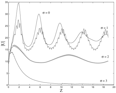
Figure 4: The evolution of the FF amplitude for 3D solitons with $\gamma=15,\delta=-0.1$ and various values of the GVD parameter $\sigma$. The soliton is generated from a Gaussian pulse launched in the FF component. It exists up to $\sigma=3$.

The realistic model must include GVM. A previous work Mihalache99a addressed “walking” STSs, but in the case $\delta>0$. Starting with a Gaussian pulse in the FF component, we tried to generate STSs with a finite GVD parameter $\sigma$. Figure 4 shows the result: at large $\gamma$ and relatively large negative $\delta$, the bullet self-traps and is found to be fully localized for moderate values of $\sigma$. The pulse cannot self-trap (decaying into radiation) if $\sigma>2$. The stability diagram displayed in Fig. 2 can be extended, adding $\sigma$ as a parameter. For $\sigma\,\,_{\sim}^{<}\,\,1$, the stability region is nearly the same as at $\sigma=0$, but with the increase of $\sigma$, it quickly shrinks and no longer exists for $\sigma>2$.

Lastly, stationary 3D solitons with an internal vorticity were found too. However, they are always unstable against perturbations breaking their axial symmetry, similar to what was found for the same type of STS in the case $\delta>0$ Mihalache2000 .

In conclusion, we have shown in the numerical form that 2D and 3D stable spatiotemporal solitons exist in quadratically nonlinear media when the dispersion is anomalous at FF but normal at SH. An exponential analytical estimate for the existence of the solitons was obtained. The solitons readily self-trap from a Gaussian pulse launched at FF, showing no trace of decay over extremely long propagation distance. The solitons have the energy smaller than their counterparts in the case of the anomalous dispersion at SH, and they exhibit robustness to the walkoff between the harmonics. These features imply that the solitons of this type can be created under a variety of experimental conditions.

We appreciate a valuable discussion with D. Mihalache and K. Beckwitt. The work was supported in a part by the Binational (US-Israel) Science Foundation (contract No. 1999459) and by a matching grant from the Tel Aviv University (TAU). Access to supercomputing facilities was provided by the High Performance Computing Unit at TAU.

References

- (1) Y. Silberberg, Opt. Lett. 15, 1281 (1990).
- (2) G.I. Stegeman and M. Segev, Science 286, 1518 (1999).
- (3) R. Schiek, Y. Baek, and G.I. Stegeman, Phys. Rev. E53, 1138 (1996).
- (4) W.E. Torruellas et al., Phys. Rev. Lett. 74, 5036 (1995).
- (5) X. Liu, L.J. Qian, and F.W. Wise, Phys. Rev. Lett. 82, 4631 (1999); X. Liu, K. Beckwitt, and F.W. Wise, Phys. Rev. E61, R4722 (2000); X. Liu, K. Beckwitt, and F.W. Wise, Phys. Rev. Lett. 85, 1871 (2000).
- (6) R. McLeod, K. Wagner, and S. Blair, Phys. Rev. A52, 3254 (1995).
- (7) J.J. Rasmussen and K. Rypdal, Phys. Scripta 33, 481 (1986).
- (8) A.B. Blagoeva et al., IEEE J. Quantum Electron. QE-27, 2060 (1991).
- (9) H.S. Eisenberg et al., Phys. Rev. Lett. 87, 043902 (2001).
- (10) C. Etrich et al., Progr. Opt. 41, 483 (2000); A.V. Buryak et al., Phys. Rep. 370, 63 (2002).
- (11) A.A. Kanashov and A.M. Rubenchik, Physica D 4, 122 (1981).
- (12) D.V. Skryabin and W.J. Firth, Opt. Commun. 148, 79 (1998).
- (13) B.A. Malomed et al., Phys. Rev. E56, 4725 (1997).
- (14) D. Mihalache et al., Opt. Commun. 152, 365 (1998); D. Mihalache et al., Opt. Commun. 159, 129 (1999).
- (15) D. Mihalache et al., Opt. Commun. 169, 341 (1999); D. Mihalache et al., Phys. Rev. E62, 7340 (2000).
- (16) D. Mihalache et al., Phys. Rev. E 62, R1505 (2000).