On Breaking Time Reversal in a Simple, Smooth, Chaotic System

Abstract

Within random matrix theory, the statistics of the eigensolutions depend fundamentally on the presence (or absence) of time reversal symmetry. Accepting the Bohigas-Giannoni-Schmit conjecture, this statement extends to quantum systems with chaotic classical analogs. For practical reasons, much of the supporting numerical studies of symmetry breaking have been done with billiards or maps, and little with simple, smooth systems. There are two main difficulties in attempting to break time reversal invariance in a continuous time system with a smooth potential. The first is avoiding false time reversal breaking. The second is locating a parameter regime in which the symmetry breaking is strong enough to transition the fluctuation properties fully toward the broken symmetry case, and yet remain weak enough so as not to regularize the dynamics sufficiently that the system is no longer chaotic. We give an example of a system of two coupled quartic oscillators whose energy level statistics closely match those of the Gaussian unitary ensemble, and which possesses only a minor proportion of regular motion in its phase space.

Since its introduction into nuclear physics by Wigner wigner , random matrix theory (RMT) has grown to encompass a broad variety of applications, and can be viewed as a significant portion of the foundation of the statistical mechanics of finite systems. One of the central tenets of RMT emphasized by Wigner was that the ensembles carry no information other than that required by the symmetries of the system. A very important symmetry is time reversal which determines whether the ensemble is composed of real symmetric matrices, Gaussian orthogonal ensemble (GOE - good symmetry), or complex hermitian matrices, Gaussian unitary ensemble (GUE - broken symmetry). This distinction leads to quite different predictions for the statistical properties of both the energy levels and the eigenfunctions. In fact, Wigner proposed it as a test of time reversal invariance in the strong interaction using slow neutron resonance data tri . His suggestion was not fully realized until more than twenty years later fkpt .

Time reversal is well known to be an antiunitary symmetry in quantum mechanics, and Robnik and Berry generalized the criterium for expecting the statistical properties of the GOE to include any antiunitary symmetry rb . An elementary example of an antiunitary symmetry would be the product of some reflection symmetry and time reversal. Some of the early investigations of noninvariant systems were of Aharanov-Bohm chaotic billiards br , symmetry breaking quantum maps izrailev ), and combinations of magnetic and scalar forces selig .

There is no known mechanical-type system of a particle moving under the influence of a simple, closed, smooth potential whose dynamics is rigorously proven to be fully chaotic, independently of the question of anti-unitary symmetry; we exclude diffusive dynamics associated with random potentials. For some period of time, the $x^{2}y^{2}$ quartic potential was a prime candidate, but eventually stable trajectories were found swedes . Nevertheless, there exists a family of quartic potentials with $x^{2}y^{2}$ as a limiting case whose fluctuations closely approximate GOE statistics, and whose classical dynamics contain negligible phase space zones of stable trajectories. Therefore,to construct a close approximation of a Hamiltonian without an anti-unitary symmetry and GUE statistics, we begin by considering the symmetry preseverving two-degree-of-freedom coupled quartic oscillators whose Schrödinger equation is given by

$$\hat{H}_{0}\Psi(\vec{r})=-{\hbar^{2}\nabla^{2}\over 2m}\Psi(\vec{r})+\hat{V}(\vec{r})\Psi(\vec{r})=E\Psi(\vec{r})$$ (1)

The potential can be expressed as

$$\hat{V}(\vec{r})=a(\lambda)\left[{x^{4}\over b}+by^{4}+2\lambda x^{2}y^{2}\right]$$ (2)

where $a(\lambda)$ is a convenient constant, $b\neq 1$ lowers the symmetry, and $\lambda$ gives the strength of the coupling; $(b=1,\lambda=-1)$ is equivalent to $V(\vec{r})=x^{2}y^{2}$ by a $\pi/4$ rotation of the $(x,y)$ coordinates. The corresponding classical Hamiltonian is

$$H_{0}(\vec{r},\vec{p})={\vec{p}^{2}\over 2m}+V(\vec{r})$$ (3)

This system is symmetric under time reversal and reflections with respect to $x$ and $y$. For strong couplings, $\lambda\leq-0.6$, the statistics have been shown to agree extremely well with the GOE predictions btu . As a first attempt to break time reversal symmetry, we add the following term to the quantum Hamiltonian ($\hat{H}=\hat{H}_{0}+\hat{H}_{1}$),

$$\hat{H}_{1}={i\hbar\epsilon\over 2m}\left(r{\partial\over\partial r}r+{\partial\over\partial r}r^{2}\right)$$ (4)

where $r$ is the radial polar variable. $\hat{H}_{1}$ breaks time reversal invariance in the Hamiltonian without altering the original reflection symmetries, and thus does not admit an antiunitary symmetry from any combination of reflection and time reversal. This term was chosen to maintain a scaling property of the eigensolutions of the quartic oscillators due to the homogeneity of the potential btu . However, $\hat{H}_{1}$ gives us an excellent example of false symmetry breaking. In fact, it turns out that $\hat{H}_{1}$ is given by the cross terms arising from a vector potential ${\bf A}(\vec{r})=\epsilon r^{2}\hat{r}$ (which can also be expressed as the gradient of a scalar function); i.e.

$$\hat{H}_{1}={i\hbar\over 2m}\left(\nabla\cdot{\bf A}(\vec{r})+{\bf A}(\vec{r})\cdot\nabla\right)$$ (5)

This means that, up to the addition to the potential of a term $\epsilon^{2}r^{4}$, $H_{1}$ can be understood as deriving from a magnetic field ${\bf B}=\nabla\times{\bf A}=0$, which obviously will not change any physical quantity. And indeed, it is possible to make a gauge transformation and rewrite the wave function using the Dirac substitution

$$\Psi(\vec{r})=\exp\left({i\over\hbar}\int^{\vec{r}}{\bf A}(\vec{r}^{\prime})\cdot{\rm d}\vec{r}^{\prime}\right)\Psi^{\prime}(\vec{r})={\rm e}^{ir^{3}\over 3\hbar}\Psi^{\prime}(\vec{r})$$ (6)

in order to cancel $\hat{H}_{1}$ plus the aforementioned $\epsilon^{2}r^{4}$ term. Furthermore, the transformation is single valued since ${\bf B}=0$ implies

$$\oint{\bf A}(\vec{r}^{\prime})\cdot{\rm d}\vec{r}^{\prime}=0\;.$$ (7)

The expectation, following the considerations of rb , is therefore to find GOE statistics and not those of the GUE. See the upper panel of Fig. (1), which compares the number variance of the system (i.e. the variance of the number of levels found in an energy interval of width $s$ scaled locally to mean unit level density) with the predictions of the GOE and GUE.

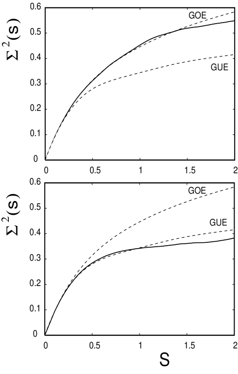
Figure 1: The number variance for the quartic oscillators (solid lines) compared to the GOE and GUE (dashed lines). The upper panel shows the statistics for the hidden symmetry case, i.e. with the Hamiltonian term in Eq. (4)) with $(\epsilon=0.5,\lambda=-0.65)$. The lower panel shows the results using the Hamiltonian term of Eq. (11) and $(\epsilon=1.0,\lambda=-0.80)$. Spectra containing a total of $600$ levels were used to generate the statistics. The lowest $50$ eigenvalues were dropped.

The GOE statistics are closely matched to a mean level spacing and a bit beyond. The parameter $\epsilon$ was chosen slightly greater than unity because this forced the eigenlevels through a couple of avoided crossings, which would have been sufficient to push the spectral fluctuations toward GUE if the symmetry was not being falsely broken.

From a classical perspective, the Hamiltonian, not incorporating the jauge transformation, is

$$H(\vec{r},\vec{p})={p_{r}^{2}-2\epsilon r^{2}p_{r}\over 2m}+{p_{\theta}^{2}\over 2mr^{2}}+V(r,\theta)$$ (8)

which itself appears to violate time reversal symmetry, as well as in Hamilton’s equations of motion:

$$\dot{r} = {1\over m}(p_{r}-\epsilon r^{2})\hskip 40.00006pt\dot{p}_{r}=-{\partial V(r,\theta)\over\partial r}+2{\epsilon\over m}rp_{r}$$

$$\dot{\theta} = {p_{\theta}\over mr^{2}}\hskip 72.5001pt\dot{p}_{\theta}=-{\partial V(r,\theta)\over\partial\theta}$$

However even without considering a canonical transformation, just by converting to the Lagrangian description of the dynamics using the left hand side equations, it turns out that

$${\cal L}={1\over 2}(m\dot{r}^{2}+mr^{2}\dot{\theta}^{2})-V(r,\theta)+{\epsilon^{2}\over 2m}r^{4}+\epsilon r^{2}\dot{r}$$ (10)

The final term, which appears to break the symmetry, cannot enter the equations of motion. They are invariant under addition of any total time derivative. It is not always obvious, a priori, whether a symmetry breaking term leads to false symmetry breaking or not.

If we multiply the symmetry breaking term by any function of $\theta$, it can no longer be a total time derivative, nor can the vector potential be expressed as the gradient of a scalar function. Consider

$$\hat{H}_{1}^{\prime}={i\hbar\epsilon\over 2m}\cos^{2}\theta\left(r{\partial\over\partial r}r+{\partial\over\partial r}r^{2}\right)$$ (11)

The vector potential becomes ${\bf A}(\vec{r})=\epsilon r^{2}\cos^{2}\theta\hat{r}$, and therefore ${\bf B}=2\epsilon xy/r\neq 0$. The integrals $\int^{\vec{r}}{\bf A}(\vec{r}^{\prime})\cdot{\rm d}\vec{r}^{\prime}$ and $\oint{\bf A}(\vec{r}^{\prime})\cdot{\rm d}\vec{r}^{\prime}$ are path dependent. The Dirac substitution is not useful, and false symmetry breaking is not an issue.

Driving the eigenvalues at numerically attainable energies through a couple of avoided crossings forces $\epsilon$ to be chosen in the neighborhood of unity. This has a strong regularizing effect on the nature of the dynamics. See the surface of section in Fig. (2) for the case ($\lambda=-0.8,\epsilon=1$).

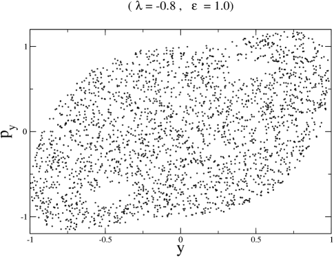
Figure 2: The $x=0$ Poincaré surface of section for the Hamiltonian with the term from Eq. (11), and parameters ($\lambda=-0.8,\epsilon=1$) as in the bottom panel of Fig. (1). The coordinates $y$ and $p_{y}$ are in scaled unit.

Only its spectrum gives number variance statistics close to the GUE results; see the lower panel of Fig. (1).

To summarize, we have given an example of a simple, continuous, dynamical system that comes close to generating GUE statistics. It is surprisingly difficult to find an essentially, fully chaotic system that does so. The pitfall of false time reversal breaking can lead to symmetries that are quite well hidden, and the addition of a vector potential to a dynamical system has a strong tendency to move the system away from fully developed chaos.

We gratefully acknowledge support from ONR grant N00014-98-1-0079 and NSF grant PHY-0098027.

References

- (1) E. P. Wigner, Ann. Phys. 67, 325 (1958), reprinted in “Statistical Theories of Spectra: Fluctuations”, (C. E. Porter, ed.), Academic Press, New York, (1965); T. A. Brody, J. Flores, J. B. French, P. A. Mello, A. Pandey and S. S. M. Wong, Rev. Mod. Phys. 53, 385 (1981).
- (2) E. P. Wigner, SIAM Rev. 9, 1 (1967).
- (3) J.B. French, V. K. B. Kota, A. Pandey, and S. Tomsovic, Ann. Phys. 181, 198 (1988); Ann. Phys. 181, 235 (1988).
- (4) M. Robnik and M. V. Berry, J. Phys. A: Math. Gen. 19, 669 (1986).
- (5) M. V. Berry and M. Robnik, J. Phys. A: Math. Gen. 19, 649 (1986).
- (6) F. M.Izrailev, Phys. Rev. Lett. 56, 541 (1986).
- (7) T. H. Seligman and J. J. M. Verbaarschot, Phys. Lett. 108A, 183 (1985).
- (8) P. Dahlqvist and G. Russberg, Phys. Rev. Lett. 65, 2837 (1990).
- (9) O. Bohigas, S. Tomsovic, and D. Ullmo, Physics Reports 223 (2), 45 (1993).