[

Universality of anisotropic fluctuations from numerical simulations of turbulent flows

Abstract

We present new results from a direct numerical simulation of a three dimensional homogeneous Rayleigh-Bénard system (HRB), i.e. a convective cell with an imposed linear mean temperature profile along the vertical direction. We measure the SO(3)-decomposition of both velocity structure functions and buoyancy terms. We give a dimensional prediction for the values of the anisotropic scaling exponents in this Rayleigh-Bénard systems. Measured scaling does not follow dimensional estimate, while a better agreement can be found with the anisotropic scaling of a different system, the random-Kolmogorov-flow (RKF) [1]. Our findings support the conclusion that scaling properties of anisotropic fluctuations are universal, i.e. independent of the forcing mechanism sustaining the turbulent flow.

] Small scales turbulent statistics is a challenging open problem for both theoretical and experimental studies in hydrodynamical systems [2]. Typical questions are connected to the understanding of the universality issue, i.e. to which extent small-scale turbulent fluctuations are statistically independent of the large-scale set-up used to inject energy in the flow. Robustness of small-scale physics cannot be exact. For instance, different forcings may inject large-scale different anisotropic fluctuations, which must have some direct/indirect influence on small-scale statistics.

A first strong requirement for universality to hold is therefore that large-scale anisotropic fluctuations becomes more and more sub-leading by going to smaller and smaller scales. In other words, at scales small enough, the omnipresent and universal isotropic fluctuations must be the leading statistical components. Such a requirement is always observed in both experiments and numerical simulations, although some subtle effects may show up due to the existence of anomalous anisotropic scaling (see [3, 1, 4, 5] for a detailed discussion of this issue). Another important question which must be asked about universality of small scales statistics, is connected to the anisotropic components on their own, independently on their comparison with the isotropic ones. In particular, it is important to understand whether the anisotropic components of any turbulent correlation functions have a scaling behavior characterized by universal exponents or not, in the limit of high Reynolds numbers.

In this Letter we present first results of an attempt to study the small-scale anisotropic behavior of a homogeneous three dimensional Rayleigh-Bénard system (HRB), i.e. a convective cell with fixed linear mean temperature profile along the vertical direction. The main focus of our analysis is a comparison between the statistical behavior of HRB system with a completely different anisotropic flow, a random-Kolmogorov-flow (RKF) [3, 1]. From the comparison, we show that the two systems have almost indistinguishable, in the limit of our numerical resolution, small-scale anisotropic (and isotropic) scalings, i.e. we find a high degree of small-scale universality for all measurable anisotropic components. This result is particularly relevant because its validity is only possible if HRB has anomalous (to be defined below in details) anisotropic small-scale fluctuations.

This Letter is organized as follows. First we briefly discuss the physics of HRB flow and the details of our numerical simulations. Second, we review the technique of SO(3) decomposition to disentangle different anisotropic contributions to any velocity correlation functions. We then present our numerical results on the HRB.

We first show that the observed anisotropic scaling is anomalous, i.e. it does not follow the dimensional predictions than can be derived by an analysis of the equation of motion. We then address in details small-scale universality by making the comparison between HRB and RKF anisotropic properties, the central point of the present Letter.

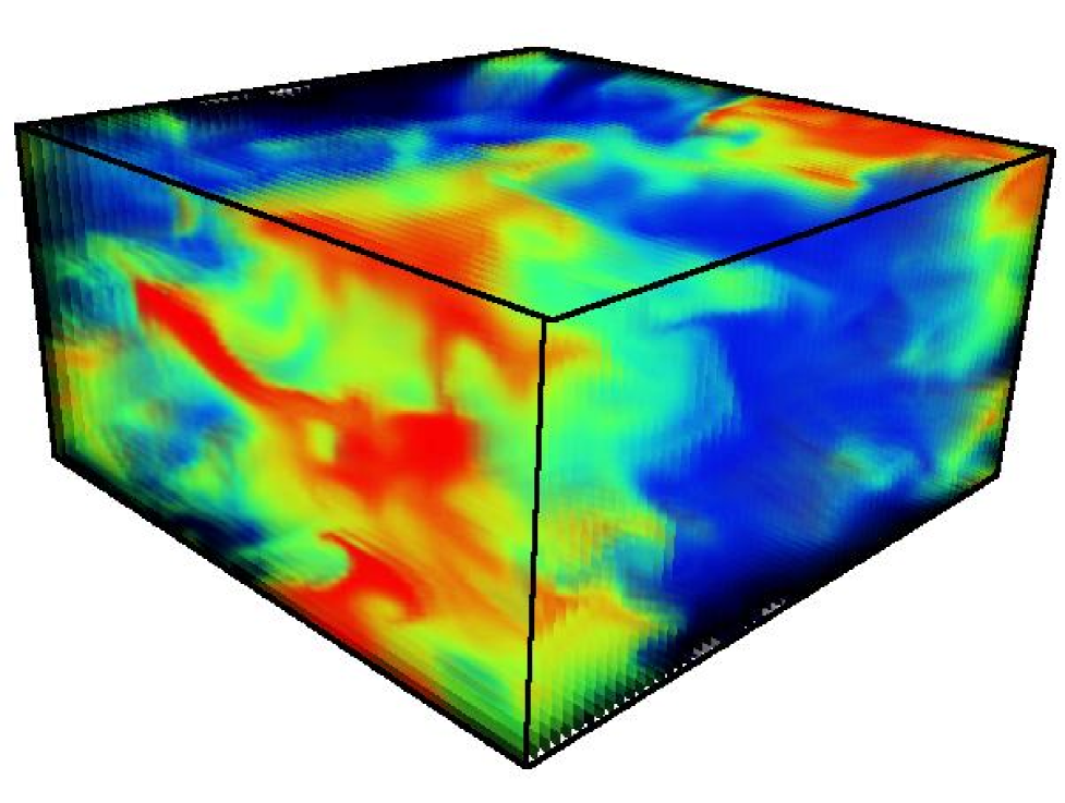
FIG. 1.: A snapshot of the temperature fluctuations in the 3D HRB system. The system is fully periodic. Notice the presence of typical convective structures [6] as the neat plume on the bottom/left of the picture.

An Homogeneous Rayleigh-Bénard system (HRB) is a convective cell with fixed linear mean temperature profile along the vertical direction. The flow is obtained by decomposing the temperature field as the sum of a linear profile plus a fluctuating part, $T(x,y,z;t)=T^{\prime}(x,y,z;t)+(\Delta T/2-z\Delta T/H)$, where $H$ is the cell height and $\Delta T$ the background temperature difference. The evolution of a HRB system can be described by a modified version [14] of the Boussinesq system [6]:

$$\partial_{t}{\mbox{\boldmath$v$}} + \left({\mbox{\boldmath$v$}}\cdot\nabla\right){\mbox{\boldmath$v$}}=-\nabla p+\nu\nabla^{2}{\mbox{\boldmath$v$}}+\alpha gT^{\prime}{{\mbox{\boldmath$\hat{z}$}}}$$ (1)

$$\partial_{t}T^{\prime} + \left({\mbox{\boldmath$v$}}\cdot\nabla\right)T^{\prime}=\kappa\nabla^{2}T^{\prime}-{{\Delta T}\over H}v_{z}.$$ (2)

Fully periodic boundary conditions are used for the velocity field, $v$, and temperature, $T^{\prime}$, fields.
For large Rayleigh numbers, HRB shows a turbulent convective dynamics with absence of both viscous and thermal boundary layers [14]. The Bolgiano scale, $L_{B}\equiv\epsilon^{5/4}N^{-3/4}(\alpha g)^{-3/2}$, is of the order of the integral scale of the cell (H), hence temperature fluctuations have a leading role only at the largest scales in the system. This has been already shown in a similar simulation [8], and is consistent with the picture presented in [7].

The main advantage of the HRB system is that the intrinsic homogeneity along the three directions allow a systematic study of scaling properties without spurious (non-homogeneous) effects, always present in standard Rayleigh-Bénard systems with boundary layers.

In order to asses the importance and properties of anisotropic components for any correlation function it is necessary to make a decomposition on the complete basis of the SO(3) group [9]. In particular, in the following, we are mainly interested in the SO(3) decomposition of scalar quantities, as for the case of velocity longitudinal structure functions, $S^{(p)}({\mbox{\boldmath$r$}})={\langle}\left[\left({\mbox{\boldmath$v$}}\left({\mbox{\boldmath$r$}}\right)-{\mbox{\boldmath$v$}}\left(0\right)\right)\cdot{\mbox{\boldmath$\hat{r}$}}\right]^{p}{\rangle}\,$:

$$S^{(p)}({\mbox{\boldmath$r$}})=\sum_{j=0}^{\infty}\sum_{m=-j}^{j}{\cal S}^{(p)}_{jm}(r)Y_{jm}({\mbox{\boldmath$\hat{r}$}});$$ (3)

where the indices $(j,m)$ label the total angular momentum and its projection on a reference axis of the spherical harmonics $Y_{jm}({\mbox{\boldmath$\hat{r}$}})$, respectively (see [9, 3] for more details). The physics is hidden in the projections, ${\cal S}^{(p)}_{jm}(r)$. We are interested to measure what are the scaling properties (if any) of each projections on different anisotropic sectors:

$${\cal S}^{(p)}_{jm}(r)\sim c_{jm}r^{\xi^{j}(p)}.$$ (4)

where we have assumed, on the basis of theoretical [9] and numerical [3] evidences, that the scaling exponents do not depend on the $m$ index. To go back to the universality issue discussed at the beginning; we expect that the coefficients $c_{jm}$ are strongly dependent on the anisotropic properties of the large-scale physics while the values of the scaling exponents, $\xi^{j}(p)$, must enjoy a much higher degree of universality. In other words, whether a particular sector is alive, $|c_{jm}|>0$, or not, $c_{jm}=0$, depends on the forcing; while, once that sector is switched-on, the way it propagates to small-scale is forcing-independent. This picture can be proved on a rigorous basis for some problems of scalar/vector advection by Gaussian, white-in-time, velocity fields (Kraichnan models [10]).
Concerning the SO(3) analysis let us notice that velocity structure functions have even parity with respect to $r$, therefore projections on odd $j$ values vanish. In the following, we consider also mixed velocity and temperature structure functions which have, on the other hand, dominant odd parity.
From equation (1) one may easily write down the stationary equation for the second order velocity structure functions; the extension of Kármán-Howarth equation in the presence of a buoyancy term [11]. The result is, neglecting for simplicity tensorial symbols:

$${\langle}\delta v({\mbox{\boldmath$r$}})^{3}{\rangle} \sim \ \ \epsilon\ r\ +\ \alpha g{\mbox{\boldmath$\hat{z}$}}r\ \cdot\ {\langle}\delta T({\mbox{\boldmath$r$}})\ \delta v({\mbox{\boldmath$r$}}){\rangle}$$ (5)

_j=0,1,… $$\ \ {}_{j=0}\quad\ \ {}_{j=1\quad\otimes\quad j=1,2,\dots}$$ (6)

where with $\epsilon$ we denote the energy dissipation and with, ${\langle}\delta v({\mbox{\boldmath$r$}})^{3}{\rangle}$ and ${\langle}\delta T({\mbox{\boldmath$r$}})\ \delta v({\mbox{\boldmath$r$}}){\rangle}$, the general third-order velocity correlation and temperature-velocity correlation, respectively. The two terms on the r.h.s. of equation (5) are called respectively the energy-dissipation term and buoyancy term. In (5) we report for each term the value of its total angular momentum, $j$. Let us notice that the energy dissipation term in (5) has a non-vanishing limit, for high Reynolds numbers, only in the isotropic sector, $j=0$. On the other hand, the buoyancy coupling, $\alpha g{\mbox{\boldmath$\hat{z}$}}$, brings only angular momentum $j=1$. Due to the usual rule of composition of angular momenta we have that the buoyancy term, $\alpha g{\mbox{\boldmath$\hat{z}$}}\cdot{\langle}\delta T({\mbox{\boldmath$r$}})\ \delta v({\mbox{\boldmath$r$}}){\rangle}$, has a total angular momentum given by the rule: $j_{tot}=1\otimes j=\{j-1,j,j+1\}$. Using the angular momenta summation rule for $j$ we can decompose the previous equation obtaining the following dimensional matching, in the isotropic sector:

$${\langle}\delta v(r)^{3}{\rangle}_{j=0}\sim\epsilon\ r+\alpha g\ {\mathbf{\hat{}}{z}}r\ {\langle}\delta v(r)\ \delta T(r){\rangle}_{j=1}+\dots$$ (7)

and in the anisotropic sectors, $j>0$:

$${\langle}\delta v(r)^{3}{\rangle}_{j}\sim\ \ \alpha g\ {\mathbf{\hat{}}{z}}r\ {\langle}\delta v(r)\ \delta T(r){\rangle}_{(j-1)}+\dots$$ (8)

where only dominant contributions are reported.

In the isotropic sector the buoyancy term is sub-dominant with respect to the dissipation term at scales smaller than the Bolgiano length, $r<L_{B}$ [12]. Therefore, in our simulation the isotropic velocity fluctuations are closer to the typical Kolmogorov scaling, $\delta v(r)\sim r^{1/3}$, rather than to the Bolgiano-Obhukhov scaling, $\delta v(r)\sim r^{3/5}$.
Let us now focus on the anisotropic sectors. Equation (8) is the simplest dimensional prediction one can derive for this system consistently with the anisotropic properties of the buoyancy term, sector by sector. It plays a key role in the following because we will show that the observed anisotropic scaling in our HRB system differ from the matching (8), i.e. we measure anomalous anisotropic scaling exponents.

Our HRB simulation was performed using a Lattice Boltzmann scheme, with spatial resolution of $240^{3}$. We stored roughly 270 statistical independent configurations. The Prandtl number for the simulation is equal to unit, and the Rayleigh number $Ra=(\alpha g\Delta TH^{3})/(\nu\kappa)=1.38\cdot 10^{7}$. Measured Bolgiano scale is $L_{B}\sim 370$, roughly one and half the cell size, while $\alpha g$ used in the equation of motion (1) is $2\cdot 10^{-3}$. A typical snapshot of the temperature field is shown in Figure 1. Notice the well detectable structures typical of all other Rayleigh-Bénard cell [6, 13, 15, 16]. In particular, there is a beautiful hot plume on the central bottom/left part of the picture.

We now present our numerical results. In order to check the small-scale properties of the HRB system we have carried out the SO(3) decomposition of both longitudinal velocity structure functions (3) up to order $p=6$ and of the simplest set of buoyancy-like terms made of $q$ velocity longitudinal increments and of one temperature increment, $B^{(q,1)}({\mbox{\boldmath$r$}})={\langle}\left[\left({\mbox{\boldmath$v$}}\left({\mbox{\boldmath$r$}}\right)-{\mbox{\boldmath$v$}}\left(0\right)\right)\cdot{\mbox{\boldmath$\hat{r}$}}\right]^{q}\left(T\left({\mbox{\boldmath$r$}}\right)-T\left(0\right)\right){\rangle}\,$:

$$B^{(q,1)}({\mbox{\boldmath$r$}})=\sum_{j=0}^{\infty}\sum_{m=-j}^{j}{\cal B}^{(q,1)}_{jm}(r)Y_{jm}({\mbox{\boldmath$\hat{r}$}}).$$ (9)

The dimensional matching made in (8) can be extended to any order of correlation function, giving, in terms of the velocity and buoyancy projections, the leading scaling contribution:

$${\cal S}^{(p)}_{jm}(r)\sim r{\cal B}^{(p-2,1)}_{j-1,m}(r).$$ (10)

Denoting with $\chi^{j}(q,1)$ the anisotropic scaling properties of the buoyancy terms, ${\cal B}^{(q,1)}_{j-1,m}(r)\sim r^{\chi^{j}(q,1)}$ we get the dimensional estimate linking velocity and buoyancy scaling:

$$\xi_{d}^{j}(p)=1+\chi_{d}^{j-1}(p-2,1)$$ (11)

where we have added a subscript $d$ to remind the reader that it is the result of a dimensional matching.

Let us first discuss the issue of anisotropic anomalous scaling by making a comparison between the numerical measurements and the dimensional estimate (11). In Fig. 2 we show a comparison between the velocity and buoyancy $j=4$ projections for $p=3,5$.

FIG. 2.: Log-log plot of quantities entering in the dimensional matching (10) for some anisotropic sectors vs $r$. Two top curves refer to ${\cal S}^{(p)}_{j,0}(r)$ ($\ast$) and to the buoyancy term $r{\cal B}^{(p-2,1)}_{j-1,0}(r)$ ($\square$) with $p=3$ and $j=4$. The two bottom curves refer to the case $p=5$ with symbols, ($+$) for the velocity projection and ($\times$) for the buoyancy term. Inset: same for $j=6$. Notice that the buoyancy term decays faster in all cases. In both plots, buoyancy terms are shifted along $y$-axis for the sake of presentation and we limited the $r$-range extension to those values with a statistically significant signal.

The inertial scaling measured for the projection of the velocity structure function, ${\cal S}^{(p)}_{jm}(r)$, is more intermittent than the corresponding buoyancy term, $r{\cal B}^{(p-2,1)}_{j-1,m}(r)$. In other words, the observed velocity scaling is different from the dimensional matching derived from the equations of motion: it is anomalous. This result holds for all measurable orders also for $j=2$ and for $j=6$ sector ($j=6$ is shown in the inset).

Let us now discuss the other important issue of universality. We argue that not only HRB has anomalous anisotropic scaling but also that the measured behavior is indistinguishable from what measured in the random-Kolmogorov-flow [3]. The point is far from being trivial and must not be underestimated. The HRB has an anisotropic forcing, given by the buoyancy term, which acts at all scales, $\sim g{\mbox{\boldmath$\hat{z}$}}\delta T(r)$, i.e. there is also a direct inject of anisotropies at small-scale, at variance with the RKF where the forcing was only at large scales. In Fig. (3) we show an overall comparison of ${\cal S}^{(p)}_{jm}(r)$ measured on the HRB and on the RKF [3]. Comparison is limited to $j=4$ and $j=6$, because RKF data from the simulation of [3] have a sign inversion in the $j=2$ sector which makes comparison inconclusive. As can be seen the agreement is quite satisfactory, except for the very small scales, smaller then the viscous scale, where as usual the SO(3) decomposition suffers from interpolation errors. The small discrepancies at large scales are also to be expected: the inertial properties of the two flows have to match quite different conditions at large scale.

FIG. 3.: Log-log plot of anisotropic $j=4$ projections ${\cal S}^{(p)}_{j,0}(r)$ vs $r$ for both HRB and RKF flows. Each couple of –almost– coinciding curves refer to the comparison of HRB and RKF projections at a given order $p=3,4,5,6$ (top to bottom). Inset: same for $j=6$.

The same comparison for $j=6$, shown in the inset, qualitatively supports the same result.

The fact that inertial-scales fluctuations of both flows are almost indistinguishable is the first important confirmation of the universality of anisotropic fluctuations in sectors with $j=4,6$. Similar conclusions can be drawn for the $j=2$ sector in different experimental set-up [5, 17, 18] (the only sector measurable, indirectly, in experiments).

Let us conclude by summarizing the two main results of this Letter. First, anisotropic fluctuations in Rayleigh-Bénard systems are anomalous. Second, notwithstanding the direct influence of the forcing mechanism at all small-scale, anisotropic fluctuations are universal, i.e. the small-scale dynamics is dominated by anomalous fluctuations, coming from the self-organization of the inertial evolution. Similar behavior is at the origin of anomalous scaling in Kraichnan models of passive/vector advection as already discussed in the introduction. In the latter case, one connects rigorously the anomalous inertial scaling with the existence of zero-modes of the inertial operator (see for example [19, 20] for a detailed analysis of anisotropic scaling in passive advection of scalar and vector quantities, respectively). Here, for Navier-Stokes equation, one may only stress the striking similarities, without being able to push it to some rigorous statement. Concerning universalities for the isotropic scaling of this Rayleigh-Bénard system, we notice that due to the large value of the Bolgiano scale –of the order of the system size– we expect to observe small-scale isotropic fluctuations close to the usual Kolmogorov 1941 scaling (plus intermittency). This is indeed the case. The Bolgiano-Obhukhov isotropic regime with $\delta v(r)\sim r^{3/5}$ cannot be accessed from this simulation. In the framework of the dimensional matching (7) the existence of a Bolgiano-Obhukhov scaling in the isotropic sector corresponds to a leading influence of the buoyancy term in the scaling range [21].

We acknowledge useful discussion with A. Lanotte. This research was supported in part by the EU under the Grant No. HPRN-CT 2000-00162 “Non Ideal Turbulence” and by the INFN (through access to the APEmille computer resources). E. C. has been supported by Neuricam spa (Trento, Italy) in the framework of a doctoral grant program with the University of Ferrara.

REFERENCES

- [1] L. Biferale, I. Daumont, A. Lanotte, and F. Toschi, Phys. Rev. E. 66 056306 (2002).
- [2] U. Frisch, “Turbulence – The legacy of A. N. Kolmogorov”, Cambridge. Univ. Press (1995)
- [3] L. Biferale and F. Toschi, Phys. Rev. Lett. 86 4831 (2001).
- [4] L. Biferale and M. Vergassola, Phys. Fluids 13 , 2139 (2001).
- [5] X. Shen and Z. Warhaft, Phys. Fluids 12, 2976 (2000); X. Shen and Z. Warhaft, Phys. Fluids 14, 370 (2002); X. Shen and Z. Warhaft, Phys. Fluids 14, 2432 (2002).
- [6] L. Kadanoff, “Turbulent Heat Flow: Structures and Scaling”, Physics Today, 54 No. 8 (2001) 34.
- [7] E. Calzavarini, F. Toschi, and R. Tripiccione, Phys. Rev. E 66 016304 (2002).
- [8] V. Borue and S. A. Orszag, J. Sci. Comp. 12 305 (1996).
- [9] I. Arad, V. L’vov, and I. Procaccia, Phys. Rev. E 59, 6753 (1999).
- [10] G. Falkovich, K. Gawȩdzki, and M. Vergassola, Rev. Mod. Phys. 73, 913 (2001).
- [11] V. Yakhot, Phys. Rev. Lett. 69 769 (1992).
- [12] The scale where can be taken as an alternative definition of the Bolgiano length, see [7].
- [13] S. Grossmann and D. Lohse, Phys. Rev. E 66, 016305 (2002).
- [14] D. Lohse and F. Toschi, Phys. Rev. Lett. 90, 034502 (2003)
- [15] E. D. Siggia, Annu. Rev. Fluid Mech. 26 (1994) 137-168.
- [16] S. Ciliberto, S. Cioni, and C. Laroche, Phys. Rev. E 54 (1996) R5901-R5904.
- [17] S. Kurien and K. R. Sreenivasan, Phys. Rev. E 62 2206 (2000).
- [18] I. Arad, B. Dhruva, S. Kurien, V. S. L’vov, I. Procaccia and K. R. Sreenivasan, Phys. Rev. Lett. 81, 5330 (1998).
- [19] I. Arad, V. S. L’vov, E. Podivilov and I. Procaccia, Phys Rev. E 62, 4904 (2000).
- [20] I. Arad, L. Biferale and I. Procaccia, Phys. Rev. E 61, 2654 (2000).
- [21] L. Skrbek, J. J. Niemela, K. R. Sreenivasan, and R. J. Donnelly Phys. Rev. E 66, 036303 (2002).