Acceleration of chemical reaction by chaotic mixing

Abstract

Theory of fast binary chemical reaction, ${\cal A}+{\cal B}\to{\cal C}$, in a statistically stationary chaotic flow at large Schmidt number Sc and large Damköhler number Da is developed. For stoichiometric condition we identify subsequent stages of the chemical reaction. The first stage corresponds to the exponential decay, $\propto\exp(-\lambda t)$ (where $\lambda$ is the Lyapunov exponent of the flow), of the chemicals in the bulk part of the flow. The second and the third stages are related to the chemicals remaining in the boundary region. During the second stage the amounts of ${\cal A}$ and ${\cal B}$ decay $\propto 1/\sqrt{t}$, whereas the decay law during the third stage is exponential, $\propto\exp(-\gamma t)$, where $\gamma\sim\lambda/\sqrt{Sc}$.

A common expectation is that random advection should essentially accelerate chemical reactions in fluid phase, since it should lead to homogenization of the reaction mixtures. Then dynamics is determined by an interplay of three factors: diffusion, advection and chemical reaction rate. Typical situation realizing in chemical reactors is that chemical reaction itself is much faster than mixing and diffusion, i.e. the Damköhler number, Da, which is defined as the ratio of the mixing time to the characteristic time of the reaction 36Dam , is large. For the binary reaction this separation of temporal scales results in formation of lamellar structure, build of stripes, populated solely by one chemical. The stripes of different chemicals are separated from each other by an interface of complicated shape, and the chemicals co-exist only in the narrow interface domain where the chemical reaction occurs. The reaction is limited by diffusion in the sense that diffusion controls fluxes of the chemicals into the interfacial reaction zone 63FK ; 76Hil ; 84CO . The physical picture of the acceleration due to the random advection is that it stretches domains populated by one chemical into thin sheets, so that the chemical reaction driven by diffusion proceeds more efficiently because of an essential increase of the interface area. In this letter we explain how this general physical picture, formulated initially for unbounded flows applies to chaotic flows confined to a finite geometry.

We consider a binary chemical reaction, ${\cal A}+{\cal B}\to{\cal C}$, in a dilute solution of two chemicals. We study decay problem, with an initial distribution of the chemicals ${\cal A}$ and ${\cal B}$, created by injecting solution of one chemical, say of ${\cal A}$, into solution of the other chemical, ${\cal B}$. It is assumed that the inverse reaction ${\cal C}\to{\cal A}+{\cal B}$ is negligible, i.e. there is no back influence of ${\cal C}$ on the distribution of ${\cal A}$ and ${\cal B}$. Then molecular concentrations of the chemicals, $n_{a}$ and $n_{b}$, vary according to the following non-linear governing equations (see, e.g., Landau )

$$\partial_{t}n_{a,b}+({\bm{v}}\cdot\nabla)n_{a,b}=\kappa_{a,b}\nabla^{2}n_{a,b}-Rn_{a}n_{b}\,,$$ (1)

where $R$ is the reaction rate coefficient, ${\bm{v}}$ is the velocity of the flow, which is assumed to be incompressible ($\nabla\cdot\bm{v}=0$), $\kappa_{a,b}$ are the diffusion coefficients of the chemicals. Here, we assume that the fluid dynamics is independent of the chemical reaction, that is the velocity field does not sense changes in the chemical concentrations nor heat is released in the result of the chemical reaction. Our approach is also applicable to the case, realized in tubular chemical reactors, when the solution of the chemicals, prepared at the entrance, is then pushed through a pipe. In this case the position along the pipe plays the role of time in the decay problem.

The major question addressed in the letter is: how do the total amounts of chemicals, $N_{a,b}=\int\mbox{d}{\bm{r}}\,n_{a,b}(t,{\bm{r}})$, decay as time $t$ advances? We focus primarily on the stoichiometric case $N_{a}=N_{b}$. This case is of major interest for applications, as it allows to get pure product ${\cal C}$ (not mixed with the reagents), by the time reaction is completed. (An effect of a mismatch between $N_{a}$ and $N_{b}$ is briefly discussed later in this text.) We identify major stages of the chemical reaction and relate them to the chemicals decay in different parts of the flow. An essential part of the evolution is related to the boundary region.

We discuss mainly the case of $\kappa_{a}=\kappa_{b}=\kappa$. (It is argued later in the text that $\kappa_{a}\neq\kappa_{b}$ does not lead to significant changes in the theory.) Then one obtains a closed equation for the difference field, $n=n_{a}-n_{b}$,

$$\partial_{t}n+(\bm{v}\cdot\nabla)n=\kappa\nabla^{2}n\,,$$ (2)

from Eq. (1), i.e. one finds that $n(t,{\bm{r}})$ is a passive scalar field. Note, that $n$ has no definite sign, and that $\int\mbox{d}\bm{r}\,n=0$ in the case of perfect matching, $N_{a}=N_{b}$.

We assume that the chaotic statistically steady velocity field ${\bm{v}}(t,\bm{r})$ contains only few harmonics of the reservoir size, i.e. the flow is smooth. This regime can be realized in chemical reactors with mechanically rotating mixers or externally driven magnets stirring the fluid in the perfect mixing devices and also in the tubular reactors at moderate Reynolds numbers. (See 99BB for a discussion of the chemical engineering principles behind various reactor designs.) Complementary to its practical significance, passive scalar advection in a smooth chaotic flow is also a well studied (by both theoretical 59Bat ; 67Kra ; 94SS ; 95CFKLa ; 99BF and experimental 97WMG ; 00JCT ; 01GSb means) subfield of statistical hydrodynamics. (See also reviews 00SS ; 01FGV .) The passive scalar decay theory, developed in 99Son ; 99BF for an unbounded flow, was recently modified for bounded flows, i.e. for chaotic flows with suitable (no slip) conditions on the boundary 02CLa . Smoothness of the flow allows one to approximate the velocity difference between close points by a linear, although fluctuating in time, profile. In the bulk region, the linear profile approximation is valid for separations smaller than the system size $L$. In the periphery, i.e. close to the solid boundary (wall), the linear profile approximation is valid for velocity fluctuations on a scale smaller than distance to the boundary. An important consequence of the linear velocity profile approximation is that close Lagrangian trajectories diverge exponentially in time. The mean logarithmic rate of the nearby Lagrangian trajectories divergence defines the Lyapunov exponent of the flow, $\lambda$. Notice, that in the peripheral domain advection is essentially anisotropic, and the stretching rate along the boundary is estimated by $\lambda$, while the stretching rate in the direction normal to the boundary is significantly smaller.

We now discuss characteristic spatial scales in the problem. The size of the system, $L$, which is also the chaotic flow typical eddy scale, is the largest scale in the problem. A comparison of the advection and diffusion terms in Eq. (1) sets the dissipative scale of the flow, which in the bulk region is $r_{d}=\sqrt{\kappa/\lambda}$. We assume that the Schmidt number, $\mbox{Sc}\sim(L/r_{d})^{2}$, is large, i.e. in the asymptotically wide range of scales, $L\gg r\gg r_{d}$, advection dominates diffusion. The width of the diffusive boundary layer is estimated by $r_{bl}\sim\mbox{Sc}^{1/4}r_{d}$, i.e. $r_{bl}>r_{d}$. Yet another important scale, associated with the chemical reaction itself, is the size of the reaction zone, $r_{ch}$ (the width of the interfacial domain where the chemical reaction occurs). In the bulk region the scale is estimated by $r_{ch}=r_{d}[\lambda/(Rn_{m})]^{1/3}$, where $n_{m}$ is a typical concentration of the chemicals inside the layers. (The estimate for the width of the reaction zone should be modified near the boundary, where it appears to be larger than in the bulk.) Initially, $r_{ch}$ is much smaller than $r_{d}$ (and, consequently, than $L$); the inequality is a consequence of the $\mbox{Da}\gg 1$ assumption. (Indeed, in accordance with the definition, the Damköhler number can be estimated as $\mbox{Da}\sim Rn_{0}/\lambda$, where $n_{0}$ is a typical value of the initial chemical concentration. Thus, at $t=0$, $r_{ch}\sim\mbox{Da}^{-1/3}r_{d}$.) However, $r_{ch}$ grows as $n_{m}$ decreases. Thus even though the separation of scales is perfect initially, it eventually breaks down at the latest stage of the chemical reaction. A cartoon illustration of the scale hierarchy is shown in Fig. 1. The magnified striped structure is shown on the chart in the upper right corner of the figure. Regions populated by one chemical are single-colored. To resolve the interface domain, even stronger magnification is needed. Dependence of the chemicals concentrations on the coordinate normal to the interface is shown schematically on the chart in the lower right corner of the figure.

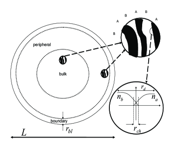
Figure 1: Chemical reactor boundary is drawn by solid line on the main chart. Dotted lines separate bulk, peripheral and boundary domains of the flow. Chart in the upper right corner shows schematically the stripe structure magnified from the bulk and/or peripheral domains. Black and white regions are the ones populated by ${\cal A}$ and ${\cal B}$ respectively. The chart in the low right corner shows (under even stronger magnified glass) distribution of chemicals normal to their contact interface.

The separation of scales, $r_{ch}\ll r_{d},L$, allows an important simplification in the description. Indeed, the chemical reaction takes place in the $r_{ch}$-narrow interface domain, where the values of $n_{a}$ and $n_{b}$ are comparable. Outside this narrow region, i.e. in the region dominated by one of the chemicals, the presence of the other chemical is negligible. Thus, in the limit $r_{ch}\to 0$, i.e. when the reaction zone becomes infinitesimally thin, one obtains $n_{a}=n,\ n_{b}=0$ for $n>0$ and $n_{a}=0,\ n_{b}=-n$ for $n<0$. These relations imply a remarkable conclusion 63FK ; 84CO : the fast chemical reaction can be described in terms of the linear setting (2) which does not contain the chemical reaction rate coefficient $R$. The reaction rate is determined by the diffusion fluxes of ${\cal A}$ and ${\cal B}$ to the $n=0$ surface. These fluxes are equal to each other and opposite in sign, which is translated, at $r_{ch}\to 0$, into a continuity condition for $\nabla n$ at the interface. This observation also means that, while $r_{ch}$ is much smaller than all other relevant scales, our problem is reduced to the problem of scalar decay in chaotic bounded flow.

Furthermore, from Eq. (2), it is straightforward to derive equations for correlation functions of $n$ (the derivation procedure is similar to the one described in 95CFKLa ; 99BF ). The equation for the mean value of $n$, $\langle n\rangle$, derived by averaging over times larger than the correlation time of the flow $\tau_{0}$, is

$$\partial_{t}\langle n\rangle=\nabla_{\alpha}(D_{\alpha\beta}\nabla_{\beta}\langle n\rangle)+\kappa\nabla^{2}\langle n\rangle\,.$$ (3)

In the case of a short-correlated (in time) flow, $\lambda\tau_{0}\ll 1$, the turbulent diffusion tensor $D$ is expressed through the velocity pair correlation function: $D_{\alpha\beta}(\bm{r})=\int_{0}^{\infty}\mbox{d}t\,\langle v_{\alpha}(t,\bm{r})v_{\beta}(0,\bm{r})\rangle$. Eq. (3) remains valid in the general, not necessarily short-correlated limit. However, the relation between the eddy-diffusivity tensor and the velocity correlations becomes more complicated. $D(\bm{r})$ tends to zero when $\bm{r}$ approaches the boundary, since the flow velocity tends to zero there. (The longitudinal component $D_{\|}$ of the tensor ${D}$ behaves as $D_{\|}\propto q^{2}$, whereas its transverse component $D_{\perp}$ behaves as $D_{\perp}\propto q^{4}$, where $q$ is the distance to the boundary.) Our description of the chemical reaction problem is based on the solutions of Eq. (3) in different spatio-temporal domains. Knowing $\langle n\rangle$, one can establish the temporal behavior of $N_{a,b}$. The brief style of this letter does not allow us to present the complete analysis here. Therefore, below we report final results, omitting details of the derivation. To clarify the results, we also pay special attention to presenting a physical picture of the phenomenon.

We find that the chemical reaction (which starts at $t=0$) undergoes the following four stages:

I. Formation of stripes in the bulk. Advection creates from an initially smooth distribution a striped structure of alternating domains of ${\cal A}$ and ${\cal B}$ 84CO . The stripes become dynamically thinner, i.e. inhomogeneities of smaller and smaller scales are produced. Once the width of the stripe decreases down to the diffusive scale, $r_{d}$, the stripe collapses (wiped out by the diffusion-limited chemical reaction) in a time $\sim\lambda^{-1}$. Since the stretching (contraction) process leading to creation of the stripes is exponential in time 59Bat ; 67Kra ; 94SS ; 95CFKLa ; 00SS ; 01FGV , the initial stage (when the $r_{d}$-stripes are formed) lasts for $\tau_{1}\sim\ln(\mbox{Sc})/\lambda$, i.e. just the time required for the cascade of passive scalar to run from $L$ down scale to $r_{d}$. Even though the interfacial area increases exponentially during the first stage, $N_{a,b}$ do not vary significantly. By the end of this stage the bulk parts of $N_{a,b}$ begin to decay rapidly (exponentially), with a decrement of the order of $\lambda$, according to the law of the passive scalar decay in an unbounded spatially smooth flow 99Son ; 99BF . Thus, after the first stage the chemicals remain mainly in the peripheral region.

Notice also, that after the first stage, stripes of different widths, distributed between $r_{d}$ and $L$, are present in the bulk. (This multi-scale structure is also seen in the passive scalar decay experiment 00JCT ; 01GSb , and in binary-reaction numerics 96ML .) When the $r_{d}$-wide stripe, say, of the chemical ${\cal A}$ collapses, then two nearby stripes of the chemical ${\cal B}$ form one wider stripe. Thus, collapse of $r_{d}$-narrow stripes is accompanied by creation of wider stripes, which are shrunk by the flow in turn, and so on and so forth.

II. Peripheral-region-dominated dynamics. The same process of layered structure formation takes place in the peripheral domain as well. However, advection, which is statistically isotropic in the bulk, is strongly anisotropic in the peripheral domain, where advection is more efficient in the direction along the boundary than in the normal direction. This anisotropy causes the layers in the peripheral domain to stretch mainly along the boundary. The stripes closer to the boundary shrink slower than the remote ones, since the normal to the boundary component of the stretching rate decreases as one approaches the boundary. Therefore the developed layered structure (i.e. the one which contains stripes of the diffusive scale width) occupies a part of the peripheral region where the amounts of $\cal A$ and $\cal B$ become negligible. Thus, the empty of chemicals region, formed in the bulk by the end of the first stage, starts to expand towards the boundary. As a result, the chemicals are arranged mainly within a $\delta$-vicinity of the boundary (wall), $\delta\sim L/\sqrt{\lambda t}$, where the concentrations of the chemicals remain practically unchanged. Outside this layer, at $L\gg q\gg\delta$ (where $q$ is the separation from the boundary), the concentration of chemicals decreases algebraically $\langle n_{a,b}\rangle\propto t^{-3/2}q^{-3}$. During this stage the overall amounts of chemicals decrease as $\delta(t)$, that is $\propto 1/\sqrt{t}$. The spatio-temporal picture explained above follows from the universal form of the velocity field profile in the proximity of the boundary. This stage lasts for $\tau_{2}\sim\sqrt{Sc}/\lambda$, i.e. until $\delta$ shrinks to the width of the boundary layer, $r_{bl}$.

III. Boundary-layer-dominated dynamics. Chemicals remain mainly within the $r_{bl}$-thin (not varying with time) vicinity of the boundary. The boundary layer width, $r_{bl}$, is still much larger than the reaction zone size (defined for the boundary region), so that the passive scalar description applies. The interfacial area where the chemicals interact does not change significantly anymore. Thus, due to linear relation between flux of chemicals to the interface and their concentrations, the algebraic decay switches to an exponential one, i.e. $\langle n_{a,b}\rangle\propto\exp(-\gamma t)$, for $t\gg\tau_{2}$, where $\gamma\sim\lambda/\sqrt{Sc}\sim L^{-1}\sqrt{\lambda\kappa}$. (Note, also, that the slow-exponential regime, derived in 02CLa for the passive scalar, is consistent with the experimental observations of 01GSb .) Then, $N_{a,b}(t)\propto\exp(-\gamma t)$. Chemicals are mainly concentrated inside the diffusion boundary layer. Outside the boundary layer (at $q\gg r_{bl}$) one of the chemicals prevails and its concentration decays algebraically, $\propto 1/q^{3}$. The passive scalar description in the vicinity of the boundary layer is broken when $r_{ch}$, which grows exponentially with time, becomes of the order of $r_{bl}$, i.e. when at the boundary $n_{a,b}$ becomes $\sim\lambda/(R\sqrt{\mbox{Sc}})$. One concludes that the duration of the boundary-layer-dominated stage is $\tau_{3}\sim\gamma^{-1}\ln(Rn_{0}\sqrt{\mbox{Sc}}/\lambda)$, where $n_{0}$ is the initial concentration of the chemicals.

IV. Nonlinear stage. By the end of the previous stage, advection and diffusion homogenize the remaining amounts of the chemicals, first, within the boundary layer and later over the entire reservoir. After that there are no inhomogeneities of $n_{a,b}$ left in the system. A purely homogeneous kinetic process takes over: $\mbox{d}N_{a,b}/\mbox{d}t=-RVN_{a}N_{b}$ (where $V$ is the chemical reactor volume). Thus, $N_{a,b}\propto 1/t$, during the final stage.

If $N_{a}\neq N_{b}$ then the proposed scheme is valid until $N_{a,b}$ become of the order of $|N_{a}-N_{b}|$. Then $N_{a}$ saturates to a constant (if $N_{a}>N_{b}$) and $N_{b}$ disappears exponentially, $\propto\exp(-RN_{a}t/V)$. (Note that the exponential decay starts after a short intermediate stage characterized by complete homogenization of ${\cal A}$ due to advection and diffusion.)

Let us now discuss the effect of unequal diffusion coefficients, still assuming that $\sqrt{\kappa_{a,b}/\lambda}\ll L$. If $\mbox{Da}\gg 1$ then during the first stages, the chemical length $r_{ch}$ is (as above) much smaller than all other scales. This problem can also be reduced to a linear one considering the advection-diffusion equations in domains populated by different species, supplemented by the condition that fluxes of the two chemicals towards the interface are equal. During the first two stages, the evolution is controlled by the stripe formation process which is insensitive to the diffusion. During the latter, third and fourth, stages of the evolution in the uneven $\kappa_{a}\sim\kappa_{b}$ case the chemicals evolve similarly to what was described above for the, $\kappa_{a}=\kappa_{b}$, case. Thus, the above description applies to the general, $\kappa_{a}\neq\kappa_{b}$, case as well.

We conclude with some general remarks. A complicated spatio-temporal behavior for the binary chemical reaction in a chaotic flow is established. Evolution of the chemicals near the boundary (where mixing is slower than in the bulk) determines the intermediate stages of the reaction. Those boundary-dominated stages were not singled out in the previous publications on the subject simply because the stages are not observed in an infinite 84CO or periodic 96ML flow systems. In our setting the lamellar structure (which is statistically isotropic in bulk and strongly anisotropic near boundaries) is dynamically generated by advection. (This situation is essentially different from the one considered in 90MO , where the lamellar structure is created initially and no advection participates in subsequent evolution.) We focused here on large scale chaotic flows with the size of the box being of the order of the major scale of the flow. However, it is also of interest for applications to describe chemical reaction acceleration in turbulent flows, which are smooth only inside the viscous range of scales. In this case with a large value of the viscous to dissipative scales ratio, a consideration similar to those presented in the letter is applicable. We plan to examine the more complicated case in the future. Also, the approach developed in the paper is generalizable for other, more complicated, types of chemical reaction, e.g. competing chemical reactions. For completeness, let us also mention another case of interest which is realized at moderate Da, large Sc and if one of chemicals is present in abundance. The joint effect of advection and chemistry is different in this case (than in the problem discussed in this letter), even though rich multi-scale structure of spatial correlations is also revealed 98Che . A final remark concerns the validity of the hydrodynamic description of the chemical reaction dynamics. It is known that the character of spatial fluctuations in the initial distribution of chemicals may essentially influence the long-time behavior in diffusion-limited chemical systems 78OZ ; 83TW . In some cases (of low space dimensionality, $d\leq 2$) large scale renormalization of the concentration fields due to the small scale fluctuations could be important. (See, e.g., 95Cara .) In our case, however, this does not happen because the long-time correlations are completely destroyed by chaotic advection.

We thank J. Cardy, G. D. Doolen, A. Fouxon, A. Groisman, I. Kolokolov, V. Steinberg, P. Tabeling, and Z. Toroczkai for helpful discussions and comments.

References

- (1) G. Z. Damköhler, Electrochem. 42, 846 (1936).
- (2) S. K. Friedlander and K. H. Keller, Chem. Engn. Sci 18, 365 (1963).
- (3) J. C. Hill, Ann. Rev. Fluid. Mech 8, 135 (1976).
- (4) R. Chella and J. M. Ottino, Chem. Eng. Sci. 39, 551 (1984).
- (5) L. D. Landau and E. M. Lifshitz, Statistical Physics, part 1, (Pergamon Press, 1980).
- (6) J. Baldyga and J. R. Bourne, Turbulent mixing and chemical reactions, John Wiley & Sons, 1999.
- (7) G. K. Batchelor, JFM 5, 113 (1959).
- (8) R. H. Kraichnan, Phys. Fluids. 10, 1417 (1967), JFM 47, 525 (1971); Ibid 67, 155 (1975).
- (9) B. I. Shraiman and E. D. Siggia, Phys. Rev. E 49, 2912 (1994).
- (10) M. Chertkov, G. Falkovich, I. Kolokolov, and V. Lebedev, Phys. Rev. E 51, 5609 (1995).
- (11) E. Balkovsky and A. Fouxon, Phys. Rev. E 60, 4164 (1999).
- (12) B. S. Williams, D. Marteau, and J. P. Gollub, Phys. Fluids 9, 2061 (1997).
- (13) M.-C. Jullien, P. Castiglione, and P. Tabeling, Phys. Rev. Lett. 85, 3636 (2000).
- (14) A. Groisman and V. Steinberg, Nature 410, 905 (2001).
- (15) B. I. Shraiman and E. D. Siggia, Nature (London) 405, 639 (2000).
- (16) G. Falkovich, K. Gawȩdzki, and M. Vergassola, Rev. Mod. Phys. 73, 913 (2001).
- (17) D. T. Son, Phys. Rev. E 59, R3811 (1999).
- (18) M. Chertkov and V. Lebedev, Phys. Rev. Lett. to appear 02/2003.
- (19) F. J. Muzzio and M. Liu, Chem. Engn. J 64, 117 (1996).
- (20) F. J. Muzzio and J. M. Ottino, Phys.Rev.A 40, 7182 (1989); 42, 5873 (1990).
- (21) M. Chertkov, Phys. Fluids 10, 3017 (1998); 11, 2257 (1999).
- (22) A. A. Ovchinnikov and Ya. B. Zeldovich, Chem. Phys. 28, 215 (1978).
- (23) D. Toussaint and F. Wilczek, J. Chem. Phys. 78, 2642 (1983).
- (24) J. Cardy, J. Phys. A: Math. Gen. 28, L19 (1995).