Fractal fractal dimensions of deterministic transport coefficients

Abstract

If a point particle moves chaotically through a periodic array of scatterers the associated transport coefficients are typically irregular functions under variation of control parameters. For a piecewise linear two-parameter map we analyze the structure of the associated irregular diffusion coefficient and current by numerically computing dimensions from box-counting and from the autocorrelation function of these graphs. We find that both dimensions are fractal for large parameter intervals and that both quantities are themselves fractal functions if computed locally on a uniform grid of small but finite subintervals. We furthermore show that there is a simple functional relationship between the structure of fractal fractal dimensions and the difference quotient defined on these subintervals.

PACS numbers: 05.45.Df, 05.45.Ac,05.60.Cd,02.70.Rr

I Introduction

Endeavours to understand fundamental laws of nonequilibrium statistical mechanics starting from the deterministic, chaotic equations of motion of a many-particle system led to the discovery of specific fractal structures forming the link between microscopic and macroscopic scales: For dissipative, so-called thermostatted systems in which deterministic transport processes such as heat or shear flow, or electric conduction, are generated by external fields, fractal attractors were claimed to be at the origin of the second law of thermodynamics [1, 2, 3]. For open Hamiltonian systems the associated repeller usually exhibits fractal properties [4, 5, 6], and in case of closed Hamiltonian systems the hydrodynamic modes of diffusion and reaction-diffusion were found to be fractal [7, 8, 9]. In all three cases the fractal dimensions of these irregular structures could be explicitly linked to the transport coefficients of the different systems [7].

Singular measures and their fractal structures in phase space were also discovered to play a fundamental role for the entropy production in simple two-dimensional area-preserving multibaker maps [5, 6, 10]. Furthermore, for a particle moving chaotically through a periodic array of scatterers the associated transport coefficients of drift, diffusion and chemical reaction were found to be irregular, typically fractal functions of control parameters [11, 12, 13, 14, 15, 16, 17, 18, 19]. However, in the latter case a detailed assessment of the irregularity of these curves in terms of fractal dimensions was not yet performed. One reason for the lack of such an analysis was the limited size of the corresponding data sets due to the fact that the precise computation of such irregular transport coefficients is generally very tedious. More recently, an exact solution became available for the irregular transport coefficients of a two-parameter piecewise linear chaotic map defined on the unit interval and periodically continued on the line [20], see Section II. In this case the explicit expressions for the diffusion coefficient and for the current were obtained in form of coupled recursion relations that converge very quickly enabling to numerically generate, in principle, arbitrarily precise and large data sets.

By using this algorithm, in this paper we analyze the structure of the parameter-dependent diffusion coefficient and of the current by numerically computing the box-counting dimension as well as the dimension related to the autocorrelation function of these graphs [21, 22]. These two methods and our numerical implementation of them are briefly described in Section III. As is well-known [13, 14, 15], the type of irregularity of these curves changes by changing the parameter: For example, in certain parameter regions the diffusion coefficient shares some features with the self-similar Koch curve, whereas in other regions it looks like a deformed Takagi function [23] or resembles some Weierstraß function [25]. This appearance of different seemingly fractal structures in different subintervals motivates us to compute dimensions not only globally for large intervals, but also locally by dividing these large intervals uniformly into a grid of small but finite subintervals. This enables us to study the dimensions as functions of the position of these subintervals. Our main result is presented in the two first parts of Section IV and states that, firstly, both transport coefficients possess fractal dimensions on large scales, and secondly, that both dimensions are fractal functions with respect to the position of the respective subintervals on which they are computed. Hence, we say that these transport coefficients are characterized by fractal fractal dimensions.

In the same section we compare the results for these two dimensions with the one obtained from a third method that amounts in computing the difference quotient of the fractal diffusion coefficient with respect to the same grid of small but finite subintervals. Previously, in case of diffusion this quantity was found to exhibit a certain structure as a function of the respective control parameter that appeared to be related to the structure of the diffusion coefficient [14]. In this paper we apply a refined analysis along these lines in parallel to our dimension computations. We find that the local difference quotient exhibits a structure that is qualitatively strikingly analogous to the functional dependence of the two local dimensions. That the two dimensions considered here are closely related to each other, though, at least in practice, quantitatively not necessarily identical, is well-known [21, 22]. However, the qualitative analogy to the difference quotient as a function of the position of the subintervals suggests a further relationship to this additional quantity which, particularly, is much more easy to compute than the two dimensions. In Section IV.C we provide a heuristic argument yielding a straightforward functional relation between the autocorrelation dimension and the difference quotient that we corroborate numerically. In Section IV.D we critically assess some subtle numerical problems related to our dimension computations, particularly by comparing our results for the transport coefficients to the ones obtained from a respective analysis of the Takagi function. We show that the latter is a fractal that does not exhibit fractal fractal dimensions and that our functional relation between the autocorrelation dimension and the difference quotient does not hold in this case. One may suspect that in this respect the fractal transport coefficients under discussion are different from self-affine fractal functions of Takagi [23], de Rham [24], or Weierstraß [25] type. Section V contains a summary of our results and lists some interesting open questions.

II A simple map with fractal transport coefficients

Simple models exhibiting deterministic diffusion are one-dimensional maps defined by the equation of motion

$$x_{n+1}=M_{a,b}(x_{n})\quad,$$ (1)

where $a,b\in\hbox{\mb R}$ are control parameters and $x_{n}$ is the position of a point particle at discrete time $n$. $M_{a,b}(x)$ is continued periodically beyond the interval $[-1/2,1/2)$ onto the real line by a lift of degree one, $M_{a,b}(x+1)=M_{a,b}(x)+1$. The map that was studied in Refs. [13, 14, 15, 20] is defined by

$$M_{a,b}(x)=ax+b\quad,$$ (2)

where $a$ stands for the slope and $b$ for the bias of the map. A sketch of this map is shown in Fig. 1. The Lyapunov exponent of this system is given by $\lambda=\ln a$ implying that for $a>1$ the dynamics is chaotic. Let $\rho_{n}(x)$ be the probability density for an ensemble of moving particles evolving according to the Frobenius-Perron continuity equation [26]

$$\rho_{n+1}(x)=\int dy\>\rho_{n}(y)\>\delta(x-M_{a,b}(y))\quad.$$ (3)

Here we are interested in the deterministic current and diffusion coefficient defined by the first and second cumulant

$$J(a,b):=\lim_{n\to\infty}\frac{1}{n}<x>$$ (4)

and

$$D(a,b):=\lim_{n\to\infty}\frac{1}{2n}(<x^{2}>-<x>^{2})\quad,$$ (5)

respectively, where the angular brackets denote an average over the probability density $\rho_{n}(x)$ as a solution of Eq. (3) for the map Eqs. (1),(2). The upper panels of all figures shown in this paper depict the parameter-dependent diffusion coefficient $D(a,b)$ or the current $J(a,b)$ of this map either as functions of $a$ for zero or fixed bias, or as functions of $b$ for fixed $a>1$. The upper curves in Figs. 1 (a) to 3 (c) were first computed in Refs. [13, 14, 15] by means of a numerical implementation of analytical (transition matrix) methods. In this paper all data sets were generated by the extremely efficient algorithm described in Ref. [20] yielding data sets that are precise up to the limits of computer precision, see this reference for further details.

In Refs. [13, 14, 15, 20] evidence was provided that all these functions exhibit a nontrivial structure on arbitrarily fine scales, which here we consider as a qualitative definition for a function to be fractal [21, 25, 27]. Partly such a behaviour was verified by producing blowups of finer and finer parameter regions constantly exhibiting irregular structures, partly parameter regimes could be detected that yielded approximately self-affine [28] structures, cp. to the upper panels of Figs. 1 to 3. The physical origin of this fractality can be traced back to the existence of long-time dynamical correlations in the deterministic dynamics of Eqs. (1),(2). A particular property of this model is that it is topologically unstable under parameter variation. That is, depending on the specific choice of parameters certain orbits may be allowed or forbidden, which in the theory of symbolic dynamics is known as “pruning” of orbits, respectively of the associated symbol sequences [29]. In Refs. [13, 14, 15] for a certain parameter interval specific series of points could be identified at which the dynamics is drastically changed related to this property. These values indeed identified approximately similar regions appearing on different scales. In case of diffusion, another approach to understand these fractal structures employs a Green-Kubo formula [18, 19, 30]. By systematically evaluating the velocity autocorrelation function of the model the diffusion coefficient can be written as a series whose single terms represent dynamical correlations of increasingly higher order. The convergence rate of this series turns out to be parameter dependent hence assessing the irregular structure of these curves. For the map under consideration, a limiting case of this approach enables to analytically relate the shape of the diffusion coefficient to de Rham-type fractal functions of which the famous Takagi function is a special case [14, 16]. However, these transport coefficients appear to be especially complicated fractals in the sense that in different parameter regions different types of fractal structures show up, cp. the upper panels of all figures. Even more, these structures do not seem to obey simple scaling laws, in contrast to Takagi, de Rham, or Weierstraß functions [23, 24, 25], which is related to the fact that their shapes are getting deformed as a function of the parameter. For the diffusion coefficient this particular property may physically be understood with respect to the Green-Kubo formula mentioned above showing that this transport coefficient emerges from two different fractal structures that are coupled to each other via integration [14, 16, 19, 30]. For the current there is only one of these two sources of fractality, however, even this one changes in a very intricate way as a function of the parameter [31] and does not appear to obey a de Rham-type functional equation [20, 24].

Thus, for the map Eqs. (1),(2) there is already quite some evidence for a non self-affine fractality of the associated transport coefficients according to the qualitative definition mentioned above. However, the irregularity of a curve can also be determined by computing dimensions such as the box-counting dimension. With respect to such quantities, a set may be called fractal if a dimension can be assigned to it which is not an integer yielding a quantitative definition of this property [21, 25, 26, 28]. In this paper we focus on assessing the irregularity of the transport coefficients of the map Eqs. (1),(2) particularly with respect to this second definition. Note that we consider both definitions only as being operational; concerning discussions about a precise definition of fractal we refer to Refs. [21, 28].

A previous computation of the box-counting dimension for the function presented in Fig. 1 (a) based on a data set of $8000$ points led to the preliminary result that this dimension should be larger than, but very close to one [14, 15]. This implies that any dimension computations are extremely delicate in order to provide evidence for a possible non-integer dimension. In the following section we briefly describe two standard methods for computing the dimension of functions as well as our approach by means of the difference quotient before in the Section IV we confirm the above statement about a non-integer dimension by applying these methods.

III Methods for assessing the structure of irregular functions

A Box-counting dimension

Let $N(\epsilon)$ be the number of squares needed to cover the graph ${G}\subset\hbox{\mb R}\times\hbox{\mb R}$ of a function $f:\hbox{\mb R}\rightarrow\hbox{\mb R}$, where $\epsilon$ is the length of one side of a square. If $N(\epsilon)$ behaves like a power law for small enough $\epsilon$, the box-counting dimension $B$ is defined as

$$B:=\lim_{\epsilon\to\infty}-\frac{\ln N(\epsilon)}{\ln\epsilon}\quad.$$ (6)

Hence, in order to compute the box-counting dimension of a function $f$ for a given interval $[c_{1},c_{2}]$ one must count the number of boxes hit by the graph $G\subset([c_{1},c_{2}]\times f([c_{1},c_{2}]))$ for a quadratic grid of grid size $\epsilon$. By successively decreasing the grid size, $B$ is obtained from the slope of a linear regression of Eq. (6). Since numerically a graph always consists of a finite number of points a double-logarithmic plot of $N(\epsilon)$ as a function of $\epsilon$ may show nonlinear behaviour in the region of small and large $\epsilon$. To find the linear portion of the resulting function is one of the crucial problems in order to minimize the computational error for the box-counting dimension; for further problems see, e.g., Refs. [21, 22, 26, 32].

We have numerically implemented this method by generating from a given graph $G$ for any $\epsilon$ a vector in which each element consists of a pair of integers referring to the coordinates of the respective box in the grid of squares that contains this point. This vector was sorted first in $x$, and if the $x$ coordinates were identical also in $y$. Then it was scanned again, and if neighbouring pairs of unequal coordinates were encountered an integer counter was increased by one.

B Dimension from the autocorrelation function of a graph

Let $f:\hbox{\mb R}\rightarrow\hbox{\mb R}$ be a continuous bounded function. If, as in our case, $f$ is only given on a finite interval $[c_{1},c_{2}]$, this function is thought to be periodically extended on ℝ. The autocorrelation function of $f$ is then defined by [21]

$$K(h)=\lim_{c\to\infty}\frac{1}{2c}\int\limits_{-c}^{c}dx\left(f(x+h)-\bar{f})(f(x)-\bar{f}\right)$$ (7)

with $\bar{f}:=\lim_{c\to\infty}1/(2c)\int_{-c}^{c}dxf(x)$ for the average value of $f$. Eq. (8) can be rewritten into

$$K(h)=K(0)-\frac{1}{2}\lim_{c\to\infty}\frac{1}{2c}\int\limits_{-c}^{c}dx(f(x+h)-f(x))^{2}$$ (8)

with $K(0):=\bar{f^{2}}-\bar{f}^{2}$. If the autocorrelation function satisfies

$$K(0)-K(h)\simeq Ch^{4-2A}$$ (9)

for small enough $h$ “it is not unreasonable to expect” the box-counting dimension $B$ to equal $A$ [21]. However, it is well-known that this is not always the case [22], hence we write the separate symbol $A$ and denote it as the autocorrelation dimension. As in case of the box-counting dimension, the term $4-2A$ can be obtained by computing $\Delta K:=K(0)-K(h)$ for successively decreasing $h$ and extracting the slope from a linear regression of this function in a double-logarithmic plot. Again, the problematic part is to identify the region of linear behaviour in order to obtain the slope of it.

Note that, in general, the box-counting dimension yields only an upper bound for the Hausdorff dimension of a graph [22], hence based on the two dimensions introduced above we cannot conclude about the Hausdorff dimension of the transport coefficients.

C Difference quotient on a grid of small but finite subintervals

Let a function $f$ be defined on the interval $[c_{1},c_{2}]\in\hbox{\mb R}$. Let us consider a grid of $n$ subintervals of size $\Delta d:=(c_{2}-c_{1})/n$ satisfying $[d_{i},d_{i+1}]\>,\>d_{i+1}:=d_{i}+\Delta d\>,\>i\in\hbox{\mb N}$, with $d_{1}=c_{1}$ and $d_{n}=c_{2}$. To any subinterval we associate a position $d_{i}+\Delta d/2$ on the parameter line. On any of these subintervals we now define the local difference quotient

$$Q_{\Delta d}(d_{i}):=\frac{f(d_{i}+\Delta d)-f(d_{i})}{\Delta d}\quad.$$ (10)

If $f$ is differentiable the limit $f^{\prime}(d_{i})=\lim_{\Delta d\to 0}Q_{\Delta d}(d_{i})$ exists. However, since fractal functions are by definition not differentiable $Q_{\Delta d}(d_{i})$ will not converge for $\Delta d\to 0$ in this case. Nevertheless, for given small but finite $\Delta d>0$ the quantity $Q_{\Delta d}(d_{i})$ is well-defined, and $Q$ as a function of $d_{i}$ may yield some information about the irregularity of $f$. Since in the following $\Delta d$ will normally be very small and held fixed we drop all indices and simplify $Q(d)\equiv Q_{\Delta d}(d_{i})$.

IV Results

We arrange our numerical results in two parts: In Section IV.A we focus on the case of zero bias $b=0$ of our model Eqs. (1),(2) for which there is only a nontrivial diffusion coefficient as a function of the slope $a$ as a parameter. Here we present results for a large parameter interval as well as for some magnifications of it. In Section IV.B we study the case of a non-zero bias $b>0$ for which, additionally, there exists a current. In this case we deal with the diffusion coefficient as well as with the current as functions of the two parameters $a$ and $b$. In Section IV.C we clarify the relation between the dimensions and the difference quotient analytically and numerically. In Section IV.D we furthermore discuss the Takagi function and argue that it shows properties that are significantly different from the ones exhibited by fractal transport coefficients.

A Diffusion coefficient for zero bias

We first quantitatively assess the irregularity of the diffusion coefficient $D(a)$ for the bias $b=0$ on the interval $2\leq a\leq 8$ as shown in Fig. 1 (a) by computing values for the box-counting dimension $B$ and the autocorrelation dimension $A$. In order to get numerically reliable values we studied the dependence of the two dimensions on the size of data sets with uniformly distributed points. For $B$ we considered up to $1000000$ data points of $D(a)$, for $A$ up to $2000000$. We found that the box-counting dimension converged quickly from below to a value of $B(D;2\leq a\leq 8)=1.039\pm 0.001$, where the numerical error denotes the maximum amplitude of the fluctuations around the asymptotic value for large enough data sets. In contrast, the autocorrelation dimension $A$ was monotonously decreasing from above by indicating slow convergence to an asymptotic value. In this case the data points were fitted by a constant plus power law and the numerical error was obtained with respect to the upper and lower bounds resulting from different fit parameters leading to $A(D;2\leq a\leq 8)=1.074\pm 0.001$. Both values are obviously not the same, however, both are very close to but different from one indicating the existence of a fractal according to our quantitative definition given in Section II. For all the other data sets presented in the following we were not able to do this tedious error analysis but computed the dimensions only for a fixed, large number of points. This implies that, because of the weak convergence of $A$ to an asymptotic value as mentioned above, results for $A$ are less reliable than for $B$.

We are now interested in the variation of these two dimensions if defined on a grid of small but finite subintervals. For this purpose we split a given large parameter interval into a large number of subintervals as described in Section IV.C. On each subinterval a data set of $1000000$ points was generated in case of $B$, and of $100000$ points in case of $A$, for which the respective dimension was computed. The dimension as a function of the position of these subintervals we may denote as the local dimension $B_{\Delta a}(a)$. First of all, Fig. 1 (b) to (d) shows that for $D(a)$ on $2\leq a\leq 8$ this function is not constant but varies irregularly with values close to one. This quantifies the observation of Refs. [13, 14, 15] that $D(a)$ exhibits different types of fractal structures in different parameter regions. However, even more Fig. 1 shows that by decreasing the size of the subintervals more and more structure in the local box-counting dimension becomes visible. This appearance of irregular structure on finer and finer scales indicates that, according to our first, qualitative definition of fractality, down to the size of the subintervals the local box-counting dimension behaves again like a fractal function. How this function evolves if the size of the subintervals goes to zero may deserve more detailed investigations that go beyond the scope of this paper. There exist lower and upper bounds for the local box-counting dimension, see also Section IV.D, however, though bounded one may strongly suspect that the limiting case of $B_{\Delta a}(a)$ for $\Delta a\to 0$ is typically not well-defined. Note furthermore the somewhat similar oscillatory behavior of $D(a)$ in Fig. 1 (a) and of the local dimension in Fig. 1 (e). Analogous results were obtained for the local autocorrelation dimension.

In Fig. 2 (b) a slightly “smoothed” version of the graph of Fig. 1 (e) is shown by having performed a running average over any three neighbouring points. This procedure was applied to most of the following local quantities in order to eliminate irregularities that may have resulted from numerical errors. Fig. 2 (c) and (d) presents respective results for the local autocorrelation dimension $A(a)$ of $D(a)$ on $2\leq a\leq 8$ shown again in Fig. 2 (a) as well as for the local difference quotient $Q(a)$ on the same subintervals according to Eq. (10). As for $Q(a)$, in the following we drop the index $\Delta a$ for $A$ and $B$, however, the respective values can be obtained from the figure captions. Fig. 2 (b) to (d) shows a striking similarity between the local box-counting dimension, the autocorrelation dimension, and the negative of the absolute value of the local difference quotient. Why we chose particularly the absolute value of $Q(a)$ will become clear in Section IV.C. The behaviour of the local difference quotient suggests a somewhat simple functional relationship between the two local dimensions and this quantity. It seems to indicate an explanation of the irregular structure of all these curves with respect to “differentiating” the original function of Fig. 2 (a) over the set of subintervals, however, as we will discuss in Section IV.D in general this interpretation has to be handled with much care. Note furthermore that on finer scales there are some systematic deviations between these three curves as can be detected, for example, by looking at the envelope of the extrema of $B(a)$ and $A(a)$ compared with $-|Q(a)|$. Note also the quantitative deviations between the local box-counting dimension and the local autocorrelation dimension.

Due to the limited data sets of $1000$ points for the graphs shown in Fig. 2 (b) and (c) together with the associated numerical errors we were not able to compute any reliable values for respective box-counting dimensions. These problems do not exist for $Q(a)$, however, here the same difficulty as we discussed for the local dimensions even more clearly shows up, namely, that this quantity is not well-defined in the limit of small subintervals. Indeed, by plotting $-|Q(a)|$ for data sets between $1000$ and $1000000$ points one observes that the local minima keep decreasing thus indicating that the structure of this curve changes profoundly with respect to the given number of subintervals. However, by trying to compute the box-counting dimensions of these different data sets we observed that, over a significant range of scales, the respective functions obeyed a power law behaviour, which enabled us to extract values for this dimension. We found that it monotonously increased from $B(-|Q(a)|;2\leq a\leq 8)\simeq 1.32$ for $1000$ points up to $B(-|Q(a)|;2\leq a\leq 8)\simeq 1.66$ for $1000000$ points. Hence, although $Q(a)$ may not be well-defined in the limiting case of infinitely small subintervals we conclude that for a finite number of subintervals and down to certain scales it exhibits characteristics of a fractal function according to our second, quantitative definition of fractality. Due to the similarity between the local dimensions and $-|Q(a)|$ one may conjecture that the same applies if the local dimensions were computed on finer and finer scales, which appears to be supported by the qualitative assessment of Fig. 1. Consequently, we say that $D(a)$ as shown in Fig. 2 (a) is characterized by a fractal fractal dimension.

Fig. 3 presents similar results for $B(a)$, $A(a)$ and $Q(a)$ on some selected subintervals of $D(a)\>,\>2\leq a\leq 8$, which exhibit different fractal structures as shown respectively in the upper panels of (a) to (c). In (a), though barely visible, there is an underlying triangular-like self-affinity that reminds a bit of a Koch curve [14]. The inset of (b) shows the plot of the Takagi function as computed from the respective functional equation [5, 6, 23], which is strictly self-similar [28] on arbitrarily fine scales. (c) may more generally remind of some Weierstraß function [25]. In case (a) the dimension computations were particularly difficult probably corresponding to the fact that for $a\to 2$ the diffusive dynamics of the model Eqs. (1),(2) approaches a random walk behaviour connected to a smooth functional dependence of the diffusion coefficient [13, 14, 15]. As for Fig. 2, we have computed the box-counting dimension for $D(a)$ on these three subintervals leading to (a) $B(D;2\leq a\leq 3)=1.021$, (b) $B(D;3\leq a\leq 3.1)=1.044$ and (c) $B(D;5.6\leq a\leq 5.7)=1.041$. The numerical error is approximately in the last digits. For the autocorrelation dimension of (a) to (c) our results indicate that $A>B$. In all these cases also the two local dimensions as well as the local difference quotient were computed, see Fig. 3, demonstrating again a considerable similarity between the structure of all these three local quantities.

B Diffusion coefficient for non-zero bias

If we choose for the map Eqs. (1),(2) a non-zero bias $b>0$ the diffusion coefficient becomes a function of two parameters $D(a,b)$. Based on stochastic theory one may not necessarily expect that a diffusion coefficient explicitly depends on the bias, however, in case of this deterministic chaotic model the nontrivial dynamical correlations mentioned in Section II cause $D$ to also be a function of $b$. Furthermore, for $b>0$ because of symmetry breaking there exists a nonzero current $J(a,b)$ that, again, is a function of the two parameters. In the upper panels of Figs. 4 to 5 we present results for the current $J(a)$ at fixed $b$ close to zero as well as for the diffusion coefficient $D(b)$ and the current $J(b)$ for $a$ close to the onset of chaos at $a=1$, where the Lyapunov exponent of the system is zero. Typically, the current is a fractal function of the two control parameters, however, as shown in Fig. 5 (b) certain parameter intervals display smooth behaviour, which is reminiscent of phase-locked dynamics in so-called Arnold tongues [20]. The inset of Fig. 5 (b) depicts a blowup of the current divided by the bias magnifying the irregular structure of the current on fine scales. The Arnold tongues also show up in the diffusion coefficient presented in Fig. 5 (a). Another interesting feature is the existence of current reversals in Fig. 4 (a), that is, depending on the slope $a$ the sign of the current is either positive or negative reminding of ratchet-like dynamics [20, 31].

As before, for Fig. 4 (a) and 5 the box-counting dimension $B$ was computed for the whole intervals displayed in these figures yielding $B(J;2\leq a\leq 8;b=0.01)=1.015$ for Fig. 4 (a), $B(D;a=1.125;0\leq b\leq 0.5)=1.021$ for Fig. 5 (a) and $B(J;a=1.125;0\leq b\leq 0.5)=1.030$ for Fig. 5 (b), with $B<A$ again in all three cases. Hence, also in the general case of two parameters both the current and the diffusion coefficient are fractal functions according to our quantitative definition of fractality.

For the current of Fig. 4 (a) as previously the two local dimensions as well as the local difference quotient were computed, see Fig. 4 (b) to (d). As far as the regions of negative currents are concerned, they do not seem to be reflected in specific properties of the corresponding local quantities. Apart from that, we observe the qualitative similarity between these three different quantities as already discussed before. This seems to confirm that there is a simple functional relationship between $B$, $A$, and the negative of the absolute value of $Q$. However, Fig. 5 clearly contradicts this statement by showing that, in these two cases, $B$ is qualitatively similar to the positive absolute value of $Q$. These results indicate that the relationship between the two local dimensions and $Q$ may indeed be more intricate asking for an explanation of this sign change. Note furthermore the similarity between $D$, $B$ and, to some extent, $|Q|$, however, compared with the previous figures it appears that, by matching the local maxima and minima, for $D$ and for $J$ there are more deviations between these different structures on finer scales than before.

C The functional relation between the autocorrelation dimension and the difference quotient

The previous figures provided numerical evidence for the existence of a relationship between the local box-counting dimension, respectively the autocorrelation dimension and the local difference quotient. As pointed out in the introduction, the relation between box-counting and the autocorrelation function is basic [21], hence it remains to clarify the relation of these two quantities to the difference quotient only. Figs. 2 to 4 show that both $B$ and $A$ are apparently similar to $-|Q|$, whereas Fig. 5 clearly tells us that these two local dimensions are similar to $+|Q|$. This puzzle will be solved in the following based on some simple analytical arguments.

We start from the observation that the autocorrelation function in form of Eq. (8) already contains the difference $\Delta f(x,h):=f(x+h)-f(x)$ for a function $f(x)$. Here we are interested in the autocorrelation function for $f$ on a small parameter interval $[d-\Delta d/2,d+\Delta d/2]$, thus we rewrite Eq. (8) in these variables and combine it with the assumed power law decay of the autocorrelation function Eq. (9) yielding

$$\frac{1}{2\Delta d}\int_{d-\Delta d/2}^{d+\Delta d/2}dx(\Delta f(x,h))^{2}=Ch^{4-2A}\quad(h\ll 1)\quad.$$ (11)

Let now in addition be $\Delta d\ll 1$ and $h\simeq\Delta d$. For small enough $\Delta d$ we approximate the average over this interval by

$$\frac{1}{\Delta d}\int_{d-\Delta d/2}^{d+\Delta d/2}dx(\Delta f(x,h))^{2}\simeq[f(d+\Delta d/2)-f(d-\Delta d/2)]^{2}\equiv(\Delta f(d))^{2}\quad(\Delta d\ll 1)$$ (12)

leading to

$$\frac{1}{2}(\Delta f(d))^{2}\simeq C(\Delta d)^{4-2A}\quad.$$ (13)

However, there is no reason why only $A$ may be a function of $d$, hence $C\equiv C(d)$, as was already remarked in Ref. [22]. By furthermore noting that $Q(d)\equiv\Delta f(d)/\Delta d$ as introduced in Eq. (10), Eq. (13) yields the important result

$$|Q(d)|\simeq\sqrt{2C(d)}(\Delta d)^{1-A(d)}\quad.$$ (14)

This equation predicts a simple relationship between the absolute value of the difference quotient $Q$ on the left hand side and a combination of $C$ and $A$ on the right hand side as functions of $d$ for fixed subinterval size $\Delta d$.

We now discuss the validity of this equation for the two cases of (i) $D(a)$ on the interval of $2\leq a\leq 8$, cp. to Figs. 1, 2, as well as for (ii) $D(b)$ on the interval $0\leq b\leq 0.5$, cp. to Fig. 5 (a). The second panels of Fig. 6 (a) and (b) from above show the local autocorrelation dimension $A$ of these two curves, the third panels the associated local difference quotient $Q$ in its original form, i.e., without taking the absolute value, whereas the lowest panels contain, among others, the respective absolute values of $Q$. Eq. (14) explains why only the absolute value of $Q$ should be related to $C$, respectively to $B$. That this is the correct solution is indeed confirmed by Fig. 6 by very carefully matching the functions depicted in the second to the fourth panels of Fig. 6 (a) to each other, say, just above $a=7$. Apart from such very fine details, the apparent constant upper bound of $A(a)$ also points to the absolute value of $Q(a)$.

More important is to understand, on the basis of this equation, this apparent “sign change” in the relation between $C$ and $|Q|$ as observed before. For this purpose we further simplify Eq. (14) in order to check whether we arrive at a simple linear relationship between these quantities as suggested by Figs. 2 to 5. We first expand the right hand side of Eq. (14) according to $(\Delta d)^{1-A}\simeq 1+(1-A)\ln(\Delta d)+\ldots$. The bounds $0\leq 1-A\leq 0.2$ and $-10\leq\ln(\Delta d)\leq-5$ obtained from the numerical data presented in our figures indicate that we can safely neglect all terms of higher order yielding

$$|Q(d)|\simeq\sqrt{2C(d)}[1+(1-A)\ln(\Delta d)]\quad.$$ (15)

For the two cases depicted in Fig. 6 we checked numerically that this equation is indeed a very good approximation. Since $\Delta d\ll 1$ and $A\geq 1$, the logarithmic term in the above equation is strictly positive. Hence, the origin of a possible “sign change” between $|Q(d)|$ and $A(d)$ can only be due to the prefactor $C(d)$. The functional dependence of $C(d)$ indeed turns out to provide the key for a complete understanding: In the upper panels of Figs. 6 (a) and (b) $C$ is plotted as a function of the respective control parameters. In both cases it obviously exhibits an irregular structure that is quite analogous to the irregular structures shown by the corresponding quantities $A$, $Q$, and $B$. Hence, $Q$ and $A$ are not the only functions in Eq. (14), respectively Eq. (15), exhibiting fractal behaviour but there is a third fractal function $C$ involved in the functional relation between them. In a way, this appears to be natural, since there is no reason why by assuming the power law Eq. (9) for the autocorrelation function and extracting a fractal local autocorrelation dimension from its exponent the respective prefactor should not also be a fractal. Fig. 6 shows that in case of the diffusion coefficient as a function of $a$ for zero bias $b=0$, i.e., if the map Eq. (2) is anti-symmetric, the oscillations of $C(a)$ are somewhat opposite to the ones of the corresponding $A(a)$, whereas in case of symmetry breaking with non-zero bias $b>0$ the oscillations of the respective function are parallel to the associated $A(b)$.

Let us first discuss the case where the oscillations of both quantities are parallel to each other, cf. to Fig. 6 (b). Then there is no mechanism inverting the oscillations on the right hand side of Eq. (15) that may mimic a minus sign. In case of Fig. 6 (a) the situation is more difficult: since the oscillations of $C(a)$ and $A(a)$ are opposite to each other it is not clear in advance which contribution dominates Eq. (15). However, a quantitative evaluation yields $1\leq A\leq 1.13$ and $-10\leq\ln(\Delta a)\leq-5$, hence $1\leq 1+(1-A)\ln(\Delta a)\leq 2.3$. On the other hand, with $0\leq C\leq 40$ it is $0\leq\sqrt{2C}\leq 9$; indeed, as shown by Fig. 6 (a), for large $a$ intervals it is $C\geq 1$. Hence, one would expect that for most intervals the first term in Eq. (15) dominates the second one indicating that the most pronounced features of $|Q(a)|$ are rather related to $C(a)$ than to $A(a)$. A look at the envelope of the largest local maxima of $C(a)$ and $Q(a)$ compared with $A(a)$ confirms this heuristic argument.

In order to assess the validity of our explanation quantitatively, the lowest panels of Fig. 6 (a), (b) display the left hand side of Eq. (14), that is, the absolute value of the respective local difference quotient $Q$, in comparison with the right hand side of this equation $P(d):=\sqrt{2C(d)}(\Delta d)^{1-A(d)}$ before linearization. Both figures show an excellent agreement of these two functions thus confirming the validity of Eq. (14). Note that in (b) the number of points of both data sets is not equal indicating that the relation between these two functions holds over a broad range of subinterval sizes $\Delta b$. The linearization Eq. (15) is indistinguishable from Eq. (14) on the scale of the figures, hence it was not included. We thus come to the conclusion that in case of the fractal transport coefficients under discussion indeed the autocorrelation dimension $A$ and the absolute value of the difference quotient $Q$ are related to each other by a simple, under certain circumstances approximately linear functional relationship. However, in addition this relation involves another fractal function, which is the prefactor of the power law Eq. (9) that is itself a fractal function of the same variable. The oscillations of this function $C$ can be either parallel or opposite to the oscillations of $A$ and hence determine whether the oscillations of $|Q|$ are in turn parallel or opposite to $A$ consequently explaining this sign change that previously was introduced ad hoc in the respective relationship.

D The Takagi function compared with the fractal diffusion coefficient

An important question is whether the results presented above are specific to these fractal transport coefficients or whether they more generally apply to self-affine fractal functions of Takagi, de Rham, or Weierstraß type. Below we discuss this point starting from the Takagi function [23] and then compare our findings with the previous results providing some insight into the problems with and limitations of assessing a curve by computing local dimensions and difference quotients.

Let us first remind of the fundamental property of monotonicity of any dimension such as box-counting, which says that if $E$ is a subset of $F$ then $dim(E)\leq dim(F)$ [21, 22]. This property poses a strict upper bound to any local dimension, which is the value of the dimension computed on the respective larger interval that got subdivided. The numbers for the box-counting dimension $B$ of the interval shown in Figs. 1, 2 and for its blowups of Fig. 3 appear to be consistent with this inequality within the bounds of numerical errors. As explained in Section IV.A, for our local $B$ we were not able to quantify the numerical error, hence this consistency check indirectly yields some indication of the size of these errors: In Figs. 1 (b) and (c), 3 (a) (which was already noted to be problematic), and 5 (a), (b) the local fluctuations significantly exceed these upper bounds indicating that all structures are mostly within the numerical errors. As was already discussed, for the local autocorrelation dimension $A$ the numerical errors are even larger. This is demonstrated by Fig. 3 where the local $A$ of the blowups partly drastically exceed the ones associated to Fig. 2 exemplifying again how delicate dimensional computations for these fractal transport coefficients are, as we already remarked to the end of Section II.

In order to understand similarities and differences between fractal transport coefficients and self-affine fractal functions we now elaborate on the dimensionality of the Takagi function depicted in the inset of Fig. 3 (b), which appears to be strikingly similar to the diffusion coefficient shown in the same figure. First of all, as is proven in Ref. [21] for the Takagi function it is exactly $B=1$. However, this value is identical with the respective lower bound for $B$, hence according to monotonicity any subinterval must also have $B=1$. Consequently, the Takagi function does not exhibit any irregularities in the local $B$. On the other hand, the local difference quotient $Q$ of the Takagi function still fluctuates irregularly due to the fact that this function is nowhere differentiable. This appears to contradict the main result of Section IV.C that there is an intimate relation between $B$ and $Q$ via $A$. However, this relation is based, among others, on the assumption that $A$ decays like a power law, see Eq. (9), whereas numerical computations for the Takagi function yield that $A$ decays exactly logarithmically. Consequently, the autocorrelation dimension is not well-defined in this case and the link between box-counting and the difference quotient breaks down.

At this point we may emphasize again that for our fractal transport coefficients such as the Takagi-like one shown in Fig. 3 (b) we unambiguously find non-logarithmic decay for the autocorrelation function corresponding to a power law for small enough variables. Further differences between both graphs of Fig. 3 (b) can be detected in the variations of the local $Q$, which in case of the Takagi function are strictly self-similar reflecting the construction of this function and which diverge symmetrically to plus and minus infinity whenever this function shows a local minimum. The local $Q$ of the diffusion coefficient, in comparison, is inherently non-symmetric, as already indicated by the lower panel of Fig. 3 (b), and diverges much more slowly to minus infinity than to plus infinity. We also did preliminary computations for the local $B$ of the Takagi function and compared them with our computations of the respective diffusion coefficient. For the Takagi function there is an extremely poor convergence to the box-counting power law Eq. (6), and if by mistake one computes local dimensions from these transient regimes one erroneously generates fluctuations of the local $B$ that look analogous to the fluctuations of the local $Q$. However, upon closer scrutiny one finds that the different functions $N(\epsilon)$ assessing the local variation of $B$ according to the prescription in Section III.A slowly converge to each other without any intersections. For our transport coefficient computations we did not observe any such peculiar convergence of these functions in case of local dimensions, instead we detected clear intersections indicating that we do not obtain local fluctuations that are due to some initial transient regime. In case of Fig. 3 (b) these differences furthermore show up in the quantitative values obtained for the local $B$, which are $1\leq B\leq 1.05$ for the Takagi function, with larger portions of $B$ being close to one, and approximately $1.02\leq B\leq 1.05$ for the diffusion coefficient.

We conclude that, although at first view the diffusion coefficient of Fig. 3 (b) resembles very much a Takagi function, the latter has significantly different dimensional properties: It is a fractal according to our qualitative definition of a fractal in Section II, whereas to our quantitative definition it provides a counterexample, since $B=1$. Furthermore, the local $B$ is simply constant, $A$ is not well-defined and hence, as far as we can tell, there is no simple functional relation between the local $Q$ and any local dimension. It might be interesting to analyze generalized Takagi functions with non-integer box-counting and autocorrelation dimensions such as the ones introduced in Refs. [21, 22] along the same lines. One may suspect that they yield further examples of self-affine fractals that do not exhibit fractal fractal dimensions and for which the simple relation to the local difference quotient suggested by Eq. (14) does not hold.

V Summary and conclusions

The goal of this paper was to assess the irregular structure of the parameter-dependent transport coefficients of a simple chaotic model system, which is a two-parameter piecewise linear map defined on the line. For computing these transport coefficients, which are the diffusion coefficient and the current as functions of the slope and of the bias of the map, we used a known numerical algorithm that is based on an exact solution of this problem [20]. The resulting data sets were evaluated by computing the box-counting dimension and the dimension related to the autocorrelation function of the respective graphs. Both quantities were computed globally for large parameter intervals as well as locally on a regular grid of small but finite subintervals yielding them as functions of the position of these subintervals. Furthermore, we computed the local difference quotient on the same set of subintervals.

Our main findings are that, firstly, both the diffusion coefficient and the current of this model are fractal functions of the two control parameters, in the quantitative sense that our numerical computations yielded box-counting and autocorrelation dimensions for them that are, except in regions of phase locking, larger than one. Secondly, we find that if both dimensions are evaluated locally and plotted as functions of the position of the respective subintervals they again exhibit nontrivial structure on finer and finer scales, which is in agreement with our qualitative definition of fractality. Computations of the box-counting dimension for the qualitatively similar local difference quotient yielded values for these local variations that were significantly larger than one. Hence, we concluded that both transport coefficients are characterized by what we called fractal fractal dimensions. Thirdly, we detected a striking qualitative similarity between the local box-counting dimension, the local autocorrelation dimension, and the local difference quotient. While the relation between box-counting and the autocorrelation function is standard, we showed by means of a simple analytical approximation that there is an additional simple functional relationship between the autocorrelation dimension and the difference quotient. This result was verified numerically. A key ingredient was the observation that not only these local quantities are fractal functions of the control parameters but that furthermore another prefactor resulting from the power law behaviour of the autocorrelation function turned out to be fractal in the same way. This enabled to explain why partly the oscillations of the local autocorrelation function and of the local box-counting dimension are opposite to the ones of the absolute value of the difference quotient while in other cases they are parallel to each other.

Finally, we applied the same analysis to the Takagi function in order to learn to which extent the fractality of physical transport coefficients is similar to, or different from, the one of self-affine fractal functions of generalized Takagi, de Rham, or Weierstraß type. We found that the Takagi function does not exhibit fractal fractal dimensions and that there is no functional relationship to the local difference quotient, in sharp contrast to our findings for the transport coefficients. As we discussed, it is extremely difficult to obtain reliable numerical results if all dimensions are close to one, however, our conclusion is that the fractal transport coefficients analyzed in this paper belong to a different class of fractal functions than the self-affine fractals of the type mentioned above. This is exemplified by these significantly different properties and may be understood with respect to the physical origin of the fractality of the transport coefficients. It would be important to further study these similarities and differences by analyzing other self-affine fractals along the same lines.

Another important, more mathematical problem concerns the limiting behaviour of both local dimensions as well as of the local difference quotient in case of fractal transport coefficients. It seems evident that, for all three quantities, the respective limiting cases for the size of the subintervals going to zero will not exist, however, it might be helpful to learn more about the specific type of the supposed non-convergence possibly by looking at lower and upper bounds for these functions in this limiting case. We furthermore remark that similar irregular dependencies of local dimensions may hold not only for the case of fractal functions but also for probability measures on fractal sets such as attractors in dissipative systems. Another direction of possible future research may concern the computation of power spectra for these fractal transport coefficients in order to learn about the frequency dependence of the fractal oscillations [21]. One may also think of applying a wavelet analysis to these functions. We finally remark that practically the local difference quotient is, of course, way easier to compute than any local box-counting or autocorrelation dimension. Although at the moment we see now straightforward way to obtain quantitative values for these two local dimensions based on computing local difference quotients, since there is no simple scaling between these different quantities, it appears that the latter yields quite some information about the structure of fractal transport coefficients. Hence, if one is primarily interested in the qualitative fluctuations of local dimensions of the transport coefficients studied in this paper the local difference quotient provides a convenient access road to first approximate results.

Acknowledgments
R.K. thanks J.Groeneveld, A.Pikovsky and M.V.Berry for inspiring remarks on this subject that partly date back already some years ago. He is indebted to K.Gelfert for very helpful hints on fractal dimensions that led to eliminating a basic error in a previous manuscript. R.K. furthermore thanks Z.Koza for interesting comments and for informing him about his parallel work on this subject. He finally acknowledges a helpful hint by J.R.Dorfman and T.Gilbert on Takagi functions and, together with T.K., thanks V.Reitmann for discussions. The work by T.K. was performed during a three-month internship at MPIPKS. Both R.K. and T.K. thank the MPIPKS for financial support of T.K. during the last stages of this project.

                 

FIG. 1.: (a) Diffusion coefficient $D(a)$ on the interval $2\leq a\leq 8$ with $2000$ data points for the one-dimensional map Eqs. (1),(2) sketched in the upper left edge with bias $b=0$ and $a$ as the slope of the map. It has a box-counting dimension of $B(D;2\leq a\leq 8)=1.039\pm 0.001$ and an autocorrelation dimension of $A(D;2\leq a\leq 8)=1.074\pm 0.001$. The box-counting dimension was furthermore computed locally on a regular grid of subintervals of size $\Delta a$. Figs. (b) to (e) depict this local dimension for $\Delta a=0.6,0.12,0.03,0.006$ as a function of the center $a$ of the subintervals. By decreasing the size of the subintervals this function is itself getting irregular on finer and finer scales. Values below one for $a\to 2$ are due to numerical errors.

FIG. 2.: (a) Diffusion coefficient $D(a)$ as in Fig. 1. (b) local box-counting dimension as in Fig. 1 (e), however, here as well as for (c) and (d) a running average was performed over any three neighbouring points. (c) local autocorrelation dimension $A(a)$, and (d) the negative of the absolute value of the local difference quotient $Q(a)$. (b) to (d) consist of $1000$ points each and define the size of the subintervals.

FIG. 3.: Diffusion coefficient $D(a)$ for some subintervals of $a$ as well as the corresponding local box-counting dimension $B(a)$, the autocorrelation dimension $A(a)$ and the local difference quotient $Q(A)$. In all cases, $D(a)$ consists of $2000$ points. The inset in (b) depicts, for comparison, the famous Takagi function. The dotted lines in the lower panels of (a) to (c) consist of $200$ points each, whereas the solid lines are respectively smoothed curves obtained from suitable running averages over the original data.

FIG. 4.: (a) Current $J(a)$ on the interval $2\leq a\leq 8$ for $b=0.01$. Note the regions of negative currents, e.g., above odd integer slopes $a$. As before, (b) depicts the local box-counting dimension $B(a)$, (c) the local autocorrelation dimension $A(a)$, and (d) minus the absolute value of the local difference quotient $Q(a)$. $J(a)$ consists of $2000$ points, the other three graphs consist of $600$ points each and are smoothed out by running averages over three neighbouring points.

FIG. 5.: The upper panel in (a) shows the diffusion coefficient $D(b)$ on the interval $0\leq b\leq 0.5$ for $a=1.125$, the respective part in (b) the current $J(b)$ for the same setting. The inset in (b) presents the current divided by the bias in order to magnify the fractal fine structure of this function. In both cases the parameter regions of zero diffusion coefficient, respectively the plateau regions of the current and the linearly decreasing regions in $J(b)/b$, correspond to Arnold tongues. The lower two panels in (a) and (b) depict the local box-counting dimension $B(b)$ as well as, in contrast to the previous figures, the positive absolute value of the local difference quotient $Q(a)$ for both transport coefficients. Both $D(b)$ and $J(b)$ consist of $2000$ points each, the other graphs consist of $600$ points each and are smoothed like Fig. 4 (b) to (c).

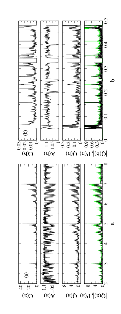
FIG. 6.: Assessing the relation between the autocorrelation dimension $A$ and the difference quotient $Q$ for two representative examples: (a) depicts the decisive quantities for the diffusion coefficient $D(a)$ on the interval $2\leq a\leq 8$, see also Figs. 1, 2, whereas (b) shows the same quantities for the diffusion coefficient $D(b)$ on $0\leq b\leq 0.5$, cp. to Fig. 5 (a). The upper panels contain results for the prefactor $C$ of the power law Eq. (9), whereas the next panels show again the local autocorrelation function obtained from the exponent of the same power law, for (a) cp. to Figs. 1 and 2. Remarkable are the irregularities of $C$ in both cases and that the oscillations are opposite to $A$ in (a), whereas they are parallel to $A$ in (b). The third panels depict again the local difference quotient $Q$, see also Fig. 2 for (a) and 5 (a) for (b). The fourth panels show a comparison between the absolute value of $Q$, which is the left hand side of Eq. (14) (black line) in comparison to the right hand side $P(a)$ of the same equation that is a function of $C$ and $A$ (grey/dotted curve). Both curves are almost indistinguishable. In (a) all curves consist of $1000$ points, in (b) the curves in the upper three panels as well as the grey curve in the fourth consist of $600$ points each. $Q(b)$ in the fourth panel is different from the one in the third panel with respect to having chosen $3000$ points.

REFERENCES

- [1] B. L. Holian, W. G. Hoover, and H. A. Posch, Phys. Rev. Lett. 59, 10 (1987).
- [2] D. Evans and G. Morriss, Statistical Mechanics of Nonequilibrium Liquids, Theoretical Chemistry (Academic Press, London, 1990).
- [3] W. G. Hoover, Time Reversibility, Computer Simulation, and Chaos (World Scientific, Singapore, 1999).
- [4] P. Gaspard and J.R. Dorfman, Phys. Rev. E 52, 3525 (1995).
- [5] P. Gaspard, Chaos, Scattering, and Statistical Mechanics (Cambridge University Press, Cambridge, 1998).
- [6] J.R. Dorfman, An Introduction to Chaos in Nonequilibrium Statistical Mechanics (Cambridge University Press, Cambridge, 1999).
- [7] T. Gilbert, J.R. Dorfman, and P. Gaspard, Nonlinearity 14, 339 (2001).
- [8] P. Gaspard, I. Claus, T. Gilbert, and J.R. Dorfman, Phys. Rev. Lett. 86, 1506 (2001).
- [9] I. Claus and P. Gaspard, Physica D 168–169, 266 (2002).
- [10] S. Tasaki and P. Gaspard, J. Stat. Phys. 81, 935 (1995).
- [11] B. Moran and W.G. Hoover, J. Stat. Phys. 48, 709 (1987).
- [12] J. Lloyd, M. Niemeyer, L. Rondoni, and G.P. Morriss, Chaos 5, 536 (1995).
- [13] R. Klages and J.R. Dorfman, Phys. Rev. Lett. 74, 387 (1995).
- [14] R. Klages, Deterministic diffusion in one-dimensional chaotic dynamical systems (Wissenschaft & Technik-Verlag, Berlin, 1996).
- [15] R. Klages and J.R. Dorfman, Phys. Rev. E 59, 5361 (1999).
- [16] P. Gaspard and R. Klages, Chaos 8, 409 (1998).
- [17] T. Harayama and P. Gaspard, Phys. Rev. E 64, 036215 (2001).
- [18] T. Harayama, R. Klages, and P. Gaspard, Phys. Rev. E 66, 026211 (2002).
- [19] N. Korabel and R. Klages, Phys. Rev. Lett. 89, 214102 (2002).
- [20] J. Groeneveld and R. Klages, J. Stat. Phys. 109, 821 (2002).
- [21] K. Falconer, Fractal geometry (Wiley, New York, 1990).
- [22] C. Tricot, Curves and fractal dimension (Springer, Berlin, 1995).
- [23] T. Takagi, Proc. Phys. Math. Soc. Japan Ser. II 1, 176 (1903).
- [24] G. de Rham, Rend. Sem. Mat. Torino 16, 101 (1957).
- [25] M.V. Berry and Z.V. Lewis, Proc. R. Soc. Lond. A 370, 459 (1980).
- [26] E. Ott, Chaos in Dynamical Systems (Cambridge University Press, Cambridge, 1993).
- [27] C. Beck and F. Schlögl, Thermodynamics of Chaotic Systems, Vol. 4 of Cambridge nonlinear science series (Cambridge University Press, Cambridge, 1993).
- [28] B. Mandelbrot, The Fractal Geometry of Nature (W.H. Freeman and Company, San Francisco, 1982).
- [29] P. Cvitanović et al., Classical and Quantum Chaos (Niels Bohr Institute, Copenhagen, 2001).
- [30] R. Klages and N. Korabel, J. Phys. A 35, 4823 (2002).
- [31] R. Klages (unpublished).
- [32] H.-O. Peitgen, H. Jürgens, and D. Saupe, Chaos and Fractals (Springer-Verlag, Berlin, 1992).
- [33] Z. Koza (private communication).