Nonlinear charge transport in DNA mediated by twist modes

Abstract

Recent works on localized charge transport along DNA, based on a three–dimensional, tight–binding model (Eur. Phys. J. B 30:211, 2002; Phys. D 180:256, 2003), suggest that charge transport is mediated by the coupling of the radial and electron variables. However, these works are based on a linear approximation of the distances among nucleotides, which forces for consistency the assumption that the parameter $\alpha$, that describes the coupling between the transfer integral and the distance between nucleotides is fairly small. In the present letter we perform an improvement of the model which allows larger values of $\alpha$, showing that there exist two very different regimes. Particulary, for large $\alpha$, the conclusions of the previous works are reversed and charge transport can be produced only by the coupling with the twisting modes.

, , and

1 Introduction

Charge transport in DNA is an interesting subject because of its role for biological functions such as DNA repair after radiation damage and biosynthesis, and, on the other hand, because of the possibility of building electronic devices based on biomaterials [1, 2, 3, 4, 5]. When a charge moves along the double DNA strand it is accompanied by a local deformation of the molecule, forming a polaron. Simple, but powerful models of DNA are based on the one proposed by Peyrard–Bishop [6], in which the only variables are the distances between bases within each base pair. The corresponding hydrogen bonds are described by Morse potentials. In the context of polaron dynamics, a tight–binding system coupled with the bond distances is used for the description of the charge dynamics. In this case, as the deformation of the helix is small a harmonic approximation of the bond potentials is considered enough giving rise to a Holstein model [7, 8].

However, the helical structure of DNA is thought to play a key role in its functional processes and recently steric models of the molecule have been introduced in the context of vibrational motion [9, 10, 11, 12, 13] and charge transport [14, 15, 16]. As it will be shown in this article, the value of the parameter $\alpha$ that couples the electronic transfer integral and the distance between nucleotides is of particular importance, determining to a great extent the degree of charge localization and its mobility properties. However there is no experimental evidence of its value. Previous works [14, 15, 16] have dealt with very small values of $\alpha$, because the angular deformations of the helix had to be small in compliance with the linear approximations performed in the expressions of the distances between nucleotides. One conclusion of these works are that charge transport in DNA is mediated by coupling of the charge carrying unit with the hydrogen–bond deformations, and that this transport survives to a small amount of parametric and structural disorder. However, we show in this work, taking into account the full equations of the model, that for larger values of $\alpha$ a completely different regime appears. In this regime charge transport is mediated by local winding and unwinding of the helix. Moreover, this regime is more robust with respect to disorder than the one mediated by the coupling with the hydrogen–bond distances.

2 The model

In order to describe the dynamic of a DNA chain, we consider a variant of the twist-opening model [9, 10, 11], which itself is a modification of the Peyrard–Bishop model taking into account the helical structure of the molecule and the torsional deformations induced by the opening of the base pairs. Each group of sugar, nucleotide and base will be considered as a single, non–deformable object, with mass $m$, which is an averaged estimation of the nucleotide mass. As we are interested in base pair vibrations and not in acoustic motions, we fix the center of mass of each base pair, $i.e.$, the two bases in a base pair are constrained to move symmetrically with respect to the molecule axis. Moreover, the distances between two neighboring base pair planes shall be treated as fixed, because in the axial direction DNA seems less deformable than within the base pair planes [9].

In our model, all bond potentials will be treated as harmonic ones. This can be justified because charge transport is related with small deformations of the double chain. Furthermore, as the angular twist and the radial vibrational motion evolve on two different time scales, they can be considered as decoupled degrees of freedom in the harmonic approximation [13]. Thus, the position of the n–th base pair is represented by the variables $(r_{n},\phi_{n})$, where $r_{n}$ represents the radial displacement of the base pair from the equilibrium value $R_{0}$, and $\phi_{n}$ its angular displacement from equilibrium angles with respect to a fixed external reference frame. A sketch of the model is shown in Fig. 1.

Figure 1: Sketch of the model. Filled circles represent bases. The variables used in the text are displayed.

The Hamiltonian of the system is given by $\widehat{H}=\widehat{H}_{el}+\widehat{H}_{rad}+\widehat{H}_{twist}$, where $\widehat{H}_{el}$ corresponds to the part related with the charged particle described by a tight–binding system: $\widehat{H}_{el}=\sum_{n}E_{n}|n\rangle\langle n|-V_{n-1,n}|n-1\rangle\langle n|-V_{n+1,n}|n+1\rangle\langle n|$, where $|n\rangle$ represents a localized state of the charge carrier at the $n^{th}$ base pair. The quantities $\{V_{n,n-1}\}$ are the nearest–neighbor transfer integrals along base pairs, and $\{E_{n}\}$ are the energy on–site matrix elements. A general electronic state is given by $|\Psi\rangle=\sum_{n}c_{n}(t)|n\rangle$, where $c_{n}(t)$ is the probability amplitude of finding the charged particle in the state $|n\rangle$. The time evolution of the $\{c_{n}(t)\}$ is obtained from the Schr$\ddot{o}$dinger equation $\mathrm{i}\hbar(\partial|\Psi\rangle/\partial t)=\widehat{H}_{el}|\Psi\rangle$

The nucleotides are large molecules and their molecular motions are slow compared to the one of a charged particle, the lattice oscillators may be treated classically and $\widehat{H}_{rad}$ and $\widehat{H}_{twist}$, describing the radial and torsional contributions to $\widehat{H}$, are, de facto, classical Hamiltonians. They are given by (omitting the hat on them):

$$H_{rad} = \sum_{n}\left[\frac{1}{2M}(p^{r}_{n})^{2}+\frac{M\Omega_{r}^{2}}{2}r_{n}^{2}\right],$$ (1)

$$H_{twist} = \sum_{n}\left[\frac{1}{2J}(p^{\phi}_{n})^{2}+\frac{J\Omega_{\phi}^{2}}{2}\ (\phi_{n}-\phi_{n-1})^{2}\right],$$ (2)

where $p^{r}_{n}$ and $p^{\phi}_{n}$ are the conjugate momenta of the radial and angular coordinates, respectively. $M=2m$ and $J=M\,R_{0}^{2}$, are the mass and the inertia moment of each base pair respectively, $\Omega_{r}$ is the linear radial frequency, and $\Omega_{\phi}$ is the linear twist frequency. We represent by $\theta_{n,n-1}=(\phi_{n}-\phi_{n-1})$, the deviation of the relative angle between two adjacent base pairs from its equilibrium value $\theta_{0}$.

The interaction between the electronic variables and the structure variables $r_{n}$ and $\phi_{n}$ arises from the dependence of the matrix elements $E_{n}$ and $V_{n,n-1}$ on them. The first ones are given by [8] $E_{n}=E_{n}^{0}+kr_{n}$, expressing the variation of the on–site electronic energies $\{E_{n}^{0}\}$ with the radial deformations. We assume that the transfer matrix elements become smaller when the distances between nucleotides grows. That is, $V_{n,n-1}$ depends on the distances between two consecutive bases along a strand as $V_{n,n-1}=V_{0}(1-\alpha d_{n,n-1})$, with $d_{n,n-1}$ given by

$$d_{n,n-1} = [a^{2}+(R_{0}+r_{n})^{2}+(R_{0}+r_{n-1})^{2}-$$ (3)

$$2(R_{0}+r_{n})(R_{0}+r_{n-1})\cos(\theta_{0}+\theta_{n,n-1})]^{1/2}-l_{0},$$

with $l_{0}=(a^{2}+4R_{0}^{2}\sin^{2}(\theta_{0}/2))^{1/2},$ and $a$ is the vertical distance between base pairs. The parameter $\alpha$ describes the influence of the distances between nucleotides on the transfer integrals. In this paper we do not perform the linear approximation of the distances $d_{n,n-1}$ considered in Refs. [15, 16], allowing for larger values of the perturbations.

Realistic parameters for DNA are given in Refs. [10, 17]. We have considered: $a=3.4\AA$, $m=300$ amu, $R_{0}=10\AA$, $\Omega_{r}=8\times 10^{12}$ s^-1, $\Omega_{\phi}=9\times 10^{11}$ s^-1, and $V_{0}=0.1$ eV. We consider $\alpha$ and $k$ as adjustable parameters.

The present model is a modification of a previous one proposed in Refs. [14, 15, 16], in order to study the transport of charge by polarons in DNA. In these works, only changes on the relative angular velocity between two neighboring base pairs, $\dot{\theta_{n,n-1}}$, are taken into account in the rotational kinetic energy, ignoring the contribution of the rest of the terms. Also, in the cited references, only very small displacements around the equilibrium position of the base pairs are considered, and the distances $d_{n,n-1}$ can be approximate by their Taylor expansion up to first order. In this paper we allow the spatial variables to have (relatively) large values and therefore we use the full nonlinear Eqs. (3) for the distances $d_{n,n-1}$.

We scale the time according to $t\rightarrow\Omega_{r}t$, and introduce the dimensionless quantities: $\tilde{r}_{n}=r_{n}\,(M\Omega_{r}^{2}/V_{0})^{1/2}$, $\tilde{k}_{n}=k_{n}/(M\Omega_{r}^{2}V_{0})^{1/2}$, $\tilde{E_{n}}=E_{n}/V_{0}$, $\tilde{\Omega}=\Omega_{\phi}/\Omega_{r}$, $\tilde{V}=V_{0}/(J\,\Omega_{r}^{2})$, $\tilde{\alpha}=\alpha\,(V_{0}/M\,\Omega_{r}^{2})^{1/2}$, $\tilde{R}_{0}=R_{0}\,(M\,\Omega_{r}^{2}/V_{0})^{1/2}$. The scaled dynamical equations of the system, from which we have omitted the tildes, are:

$$\mathrm{i}\,\tau\dot{c}_{n}=(E_{n}\,+k\,r_{n})\,c_{n}$$ (4)

$$-(1-\alpha\,d_{n+1,n})\,c_{n+1}-(1-\alpha\,d_{n\,n-1})\,c_{n-1}\,,$$

$$\ddot{r}_{n}=-r_{n}-k\,|c_{n}|^{2}$$ (5)

$$-\,\alpha\,\left[\frac{\partial d_{n,n-1}}{\partial r_{n}}(c_{n}^{*}c_{n-1}+c_{n}c_{n-1}^{*})+\frac{\partial d_{n+1,n}}{\partial r_{n}}(c_{n+1}^{*}c_{n}+c_{n+1}c_{n}^{*})\right]\,,$$

$$\ddot{\phi}_{n}=-\Omega^{2}\,(2\phi_{n}-\phi_{n-1}-\phi_{n+1})$$ (6)

$$-\,\alpha\,V\,\left[\frac{\partial d_{n,n-1}}{\partial\phi_{n}}(c_{n}^{*}c_{n-1}+c_{n}c_{n-1}^{*})+\frac{\partial d_{n+1,n}}{\partial\phi_{n}}(c_{n+1}^{*}c_{n}+c_{n+1}c_{n}^{*})\right]\,,$$

and the quantity $\tau=\hbar\,\Omega_{r}/V_{0}$ determines the time scale separation between the fast electron motion and the slow bond vibrations. In the limit case of $\alpha=0$ and uniform $E_{n}=E_{0}$ the set of coupled equations represents the Holstein system, widely used in studies of polaron dynamics in one-dimensional lattices, and for $\alpha=k=0$, and random $E_{n}$, the Anderson model is obtained. Using the expectation value for the electronic contribution to the Hamiltonian, the new Hamiltonian $\overline{H}=\langle\phi|\widehat{H}|\phi\rangle/V_{0}$ is given by

$$\overline{H} = \sum_{n}\Big{\{}\frac{1}{2}(\dot{r}_{n}^{2}+r_{n}^{2})+\frac{R_{0}^{2}}{2}[\dot{\phi_{n}^{2}}+\Omega^{2}(\phi_{n}-\phi_{n-1})^{2}]+$$ (7)

$$(E_{n}^{0}+kr_{n})|c_{n}|^{2}-(1-\alpha d_{n,n-1})(c_{n}^{*}c_{n-1}+c_{n}c_{n-1}^{*})\Big{\}}.$$

The values of the scaled parameters are $\tau=0.053$, $\Omega^{2}=0.013$, $V=2.5\times 10^{-4}$, $R_{0}=63.1$ and $l_{0}=44.5$. We fix the value $k=1$ and consider the parameter $\alpha$ as adjustable, its value complying with the hypothesis of small deformations of the helix.

3 Stationary polaron-like states

As a first step in our study of nonlinear charge transport in this DNA model, we focus our interest in localized stationary solutions of Eqs. (4-6). Since the adiabaticity parameter $\tau$ is small, the fastest variable are the $\{c_{n}\}$, with a characteristic frequency (the linear frequency of the uncoupled system) of order $1/\tau\sim 19$, followed by the $\{r_{n}\}$ with frequency unity, and the $\{\phi_{n}\}$ with $\Omega_{\phi}\sim 0.11$. Using the Born–Oppenheimer approximation, we can suppose initially that $r_{n}$ and $\phi_{n}$ are constant in order to obtain the stationary localized solutions. For this purpose, we use a modification of the numerical method outlined in Refs. [8, 18]. We substitute in Eq. (4) $c_{n}=\Phi_{n}\exp(-\mathrm{i}\,E\,t/\tau)$, with time–independent $\Phi_{n}$’s, and we obtain a nonlinear difference system $E\Phi=\widehat{A}\Phi$, with $\Phi=(\Phi_{1},...,\Phi_{N})$, from which a map $\Phi^{\prime}=\widehat{A}\Phi/\|\widehat{A}\Phi\|$ is constructed, $\|.\|$ being the quadratic norm.

Thus, using Eqs. (4-6), the stationary solutions must be attractors of the map:

$$r^{\prime}_{n}=-k\,|c_{n}|^{2}$$ (8)

$$-\,\alpha\,\left[\frac{\partial d_{n,n-1}}{\partial r_{n}}(c_{n}^{*}c_{n-1}+c_{n}c_{n-1}^{*})+\frac{\partial d_{n+1,n}}{\partial r_{n}}(c_{n+1}^{*}c_{n}+c_{n+1}c_{n}^{*})\right]\,,$$

$$\phi^{\prime}_{n}=\frac{1}{2}(\phi_{n+1}+\phi_{n-1})$$ (9)

$$-\,\frac{\alpha V}{2\Omega^{2}}\,\left[\frac{\partial d_{n,n-1}}{\partial\phi_{n}}(c_{n}^{*}c_{n-1}+c_{n}c_{n-1}^{*})+\frac{\partial d_{n+1,n}}{\partial\phi_{n}}(c_{n+1}^{*}c_{n}+c_{n+1}c_{n}^{*})\right]\,,$$

$$c^{\prime}_{n}=\frac{[(E_{n}\,+k\,r^{\prime}_{n})\,c_{n}-(1-\alpha\,d^{\prime}_{n+1,n})\,c_{n+1}-(1-\alpha\,d^{\prime}_{n\,n-1})\,c_{n-1}]}{\|\{(E_{n}\,+k\,r^{\prime}_{n})\,c_{n}-(1-\alpha\,d^{\prime}_{n+1,n})\,c_{n+1}-(1-\alpha\,d^{\prime}_{n\,n-1})\,c_{n-1}\}\|}\,,$$ (10)

where $d^{\prime}=d(r^{\prime},\phi^{\prime})$. In order to achieve convergence, it has been necessary to use the result of an interaction in the geometrical variables as a seed in the map corresponding to the probability amplitude. The starting point is a completely localized state given by $c_{n}=\delta_{n,0}$, $r_{n}=0$ and $\phi_{n}=0$, $\forall n$. The map is applied until convergence is achieved. In this way both stationary solutions and their energies $E$ are obtained.

We analyze the ordered case, i.e., $E_{n}^{0}=E_{0}$, that arises in synthetic DNA (the constant $E_{0}$ can be set to zero by means of a gauge transformation), and the disordered case. In the latter, we introduce diagonal disorder in the on–site electronic energy $E_{n}^{0}$ by means of a random potential $E_{n}^{0}\in[-\Delta E,\Delta E]$, with mean value zero and different interval sizes $\Delta E$. Such deviations can be caused by inherent disorder in the surrounding water and by the inhomogeneous distribution of counterions along the DNA duplex [19].

In the ordered case, we have found that in the ground state the charge is fairly localized at one site, and the amplitudes decay monotonically and exponentially with growing distance from the central site. The associated patterns of the static radial and relative angular displacements are similar. In the disordered case, the localized excitation patterns do not change qualitatively. However, as the translational invariance is broken by the disorder, the localized excitation pattern is not symmetric with respect to a lattice site, in opposition to the ordered case.

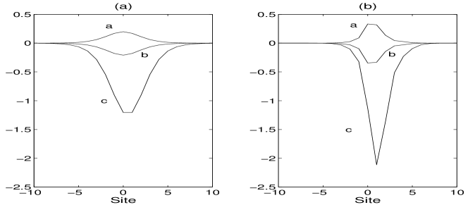
Figure 2: Profiles of the stationary state for $\alpha=0.05$. (a) Ordered case. (b) Disordered case for $\Delta E=0.01$ eV. a) Electronic probabilities $|c_{n}|^{2}$. b) Radial displacements $r_{n}$, c) Arc displacements $R_{0}\,\theta_{n,n-1}$. The displacements are in scaled units equivalent to $\simeq 0.16\AA$.

In order to study the localization of the excitation, we introduce the degree of localization $L$ of an amplitude pattern $\{u_{n}\}$ as

$$L=\frac{\sum_{n}|u_{n}|^{2}}{(\sum_{n}|u_{n}|)^{2}},$$ (11)

and the participation number $P$ as its inverse $P=1/L$. This magnitude gives an estimate of the number of excited oscillators in the chain.

We have studied the participation numbers of the electronic probabilities $|\Phi_{n}|^{2}$, the radial displacements $r_{n}$, the angular displacements $\theta_{n,n-1}$, and the density of energy as functions of the parameter $\alpha$. As Fig. 3 shows, for each given value of $\alpha$ and the disorder amplitude, the participation numbers of all these magnitudes are very close. When $\alpha$ increases, the participation decreases and therefore the localization increases. Comparing the ordered and the disordered case, we can observe that the localization is enhanced with the disorder, due to Anderson localization [20].

Figure 3: Participation number $P$ as a function of $\alpha$ for the electronic probabilities $|\Phi_{n}|^{2}$ (solid line), radial displacements $r_{n}$ (dotted line), angular displacements $\theta_{n,n-1}$ (dashed line), and density of energy (dashdot line) of the ground state for the ordered case ($\Delta E=0$) and the disordered one ($\Delta E=0.01$ eV)

4 Charge transport in the absence of disorder

In this section, we study charge transport along the double strand by moving polarons. Once a stationary state is obtained, it can be moved under certain conditions. There exists a systematic way to do it, known as the pinning mode [21], which consists of perturbing the (zero) velocities of the ground state with localized, spatially antisymmetric modes obtained in the vicinity of a bifurcation. This method leads to moving entities with very low radiation but has the inconvenience of being applicable only in the neighborhood of certain values of the parameters. Instead, we use the discrete gradient method [22], perturbing the (zero) velocities of the stationary state $\{\dot{r}_{n}(0)\}$, $\{\dot{\phi}_{n}(0)\}$ in a direction parallel to the vectors $(\nabla r)_{n}=(r_{n+1}-r_{n-1})$ and/or $(\nabla\phi)_{n}=(\phi_{n+1}-\phi_{n-1})$. Although this method does not guarantee mobility, it nevertheless proves to be successful in a wide parameter range.

4.1 Radial movability regime

In absence of diagonal disorder, and if the parameter $\alpha$ is small enough ($\alpha\lesssim 0.005$), it is not possible to move the polarons by perturbing the angular variables. Mobility can only be accomplished through perturbation of the radial ones, as in Ref. [15]. This regime is explained in detail in this reference, but, for completeness, we summarize here the most relevant characteristics:

1. The charge probability moves with uniform velocity along the lattice with apparently constant profile.

2. The movement of the charge is accompanied by a relatively large radial deformation ($r_{n}\sim 0.02\,\AA$) and a negligible angular lattice deformation ($R_{0}\theta_{n,n-1}\sim 2\cdot 10^{-5}\AA$).

3. The velocity of the polaron increases approximately in a linear way with the kinetic energy of the perturbation, as shown in Fig. 6, until a critical value, beyond which the localization is destroyed.

If we observe the spatial variables, there exists a small radial amplitude oscillation pinned at the starting site. There are radial and angular oscillations accompanying the charge and two larger angular oscillations, emerging from the same origin, that propagate in opposite directions with lower velocity than the polaron, as shown in Fig. 4.

Figure 4: Radial movability regime. Polaron motion along the chain in ordered case for $\alpha=0.0002$ and an initial kick $\lambda_{r}=0.01$ in the radial velocities, corresponding to a kinetic energy of the perturbation $\Delta K=5\times 10^{-6}$ eV. (a) Uniformly moving electronic excitation. (b) Radial displacements ($\AA$). (c) Arc displacements $R_{0}\,\theta_{n,n-1}$ ($\AA$) with $R_{0}=10\AA$.

4.2 Twist movability regime

However, for larger values of parameter $\alpha$ ($\alpha\gtrsim 0.01$), the polaron can only be moved by perturbing the angular variables. Perturbations of the radial variables cannot activate mobility. This is a consequence of the different contributions of the radial and angular components in the discrete gradient.

Figure 5: Twist movability regime. Polaron motion along the chain in ordered case for $\alpha=0.05$ and an initial kick $\lambda_{\varphi}=0.01$ in the angular velocities, corresponding to a kinetic energy of the perturbation $\Delta K=0.02$ eV. (a) Uniformly moving electronic excitation. (b) Radial displacements ($\AA$). (c) Arc displacements $R_{0}\theta_{n,n-1}$($\AA$) with $R_{0}=10\AA$.

On the twist movability regime we observe that:

1. The charge probability apparently moves with constant velocity and constant profile.

2. There are relatively large radial and angular deformations travelling with the charge ( $r_{n}\sim 0.05\,\AA$, $R_{0}\theta_{n,n-1}\sim 2\,\AA$ ).

3. The velocity of the polaron increases initially with the kinetic energy of the perturbation but tends to be approximately constant, as Fig. 6 shows. It decreases slowly with $\alpha$. This moving excitation remains localized even for large perturbations.

There remains a small radial oscillation localized at the starting site. Also an angular deformation travels with opposite direction and phase than the angular pulse moving with the charge.

Figure 6: Velocity of the polaron as a function of the kinetic energy of the perturbation $\Delta K$ added to the ground state in the ordered case. Squares correspond to the radial movability regime ($\alpha=0.0002$). Circles correspond to the mixed regime with radial activation ($\alpha=0.01$). Triangles correspond to the mixed regime with angular activation for the same value of $\alpha=0.01$. Stars correspond to the twist movability regime ($\alpha=0.05$).

4.3 Mixed regime

It is possible, for intermediates values of the parameter $\alpha$ ($0.005\lesssim\alpha\lesssim 0.01$), that the polaron can become mobile by perturbing any set of variables, the radial or the angular ones. Nevertheless, the movement is rather different as shown in Fig 6, when the polaron propagation is activated by means of radial perturbations, its characteristics are similar to the radial movability regimen, and likewise when it is activated by angular perturbations.

In general, radial movability requires less energy and has higher velocity than the angular one, as shown in Fig. 6. There exists a small interval of perturbations energies, for which the movement can be activated by means of both kind of perturbations. The velocities obtained are similar but the evolution of the spatial variables are rather different.

It is worth remarking that the limits of these regimes are not exact, depending on the kinetic energy of the perturbation, but we have intended to present a general picture.

4.4 Tail analysis of the twist movability regime

The consequences for the tail analysis of the radial movability regime has been analyzed in Ref. [16]. Here we use this simple but useful instrument to perform a similar study of the twist movability regime. The tails of the moving polaron have small amplitude and therefore their dynamics is to a great extent linear. The linear equations corresponding to Eqs. (4-6) in the ordered case are:

$$\mathrm{i}\tau\dot{c}_{n}=-c_{n+1}-c_{n-1}\,;\;\ddot{r}_{n} = -r_{n}\,;\;\ddot{\phi}_{n}=-\Omega^{2}\,(2\,\phi_{n}-\phi_{n-1}-\phi_{n+1}).$$ (12)

According to these equations, the variables $r_{n}$ are driven by the nonlinear terms and we will not consider them here. We propose the moving tail modes $c_{n}=\exp(-\xi/2\,(n-v\,t)-\mathrm{i}\,E\,t/\tau)$ and $\phi_{n}=\exp(-\xi\,(n-v\,t))$, which will be valid (relatively) far from the head of the moving polaron and while $(n-v\,t)>0$. These modes comply with the observed phenomena of similar exponential decay for $|c_{n}|^{2}$ and $\phi_{n}$ and that the second magnitude is a deformation and not an oscillation. Substitution into the first and third equations leads to:

$$\tau\,\xi\,v=4\,\sin(q)\,\sinh(\xi/2), E=-2\,\cos(q)\,\cosh(\xi/2),$$ (13)

$$\;v = 2\Omega\,\sinh(\xi/2)\,\xi^{-1}.$$ (14)

The velocity in physical units is $\tilde{v}=a\,\Omega_{r}\,v$. The inverse characteristic length can be related to the participation number by

$$P=\frac{(\sum_{n=-\infty}^{n=\infty}\exp(-\xi\,|n|))^{2}}{\sum_{n=-\infty}^{n=\infty}(\exp(-\xi\,|n|))^{2}}=\frac{\tanh(\xi)}{\tanh^{2}(\xi/2)}\,.$$

Certainly $\xi$ and $P$ are determined by the full linear equations and depend on $\alpha$, but in this way we can relate the values of $\xi$ with the numerical results for $P$. Within the twist movability regime the values of $P$ change from 5 to 12, which correspond to values for $\xi$, 0.74 and 0.33, and for $v$, 3.17 and 3.11 ($\AA/\mathrm{ps}$), respectively. For $\xi$ small, $P\sim 4/\xi$, $v\sim\Omega$ and $\tilde{v}=a\,\Omega_{r}\,\Omega=3.4\,\AA\,8\,\mathrm{ps}^{-1}\sqrt{0.013}\sim 3.1\,\AA\,\mathrm{ps}^{-1}$. The numerical results vary from 2.1 to 3.4, i.e., they are in good agreement with the values of this tail analysis, taking into account the drastic simplification of the model. Moreover, they are also coherent with the numerical observation that the velocity of the polarons practically does not depend on the kinetic energy of the perturbation, as Fig. 6 shows. The conclusion is that in this regime the polaron is basically riding on the angular wave. Equations (13) can be used to obtain the wave number $q$ and the charge energy $E$ and to compare them with the numerical data with good results, with $q\sim 6\cdot 10^{-6}$ and energies slightly below $E_{0}=-2$ (scaled units). This last value corresponds to the extended ground state with $q=0$ and $\xi=0$ [16].

5 Charge transport in the presence of disorder

If an amount of disorder in the on–site energies $E_{n}^{0}$ is introduced, with random values $|E_{n}^{0}|<\Delta E$, we find that moving polarons exist below a critical value $\Delta E_{crit}$. Beyond this value polarons cannot be moved as found in Ref. [15]. The most relevant results are:

1. In the radial movability regime, mobility is very sensitive to disorder. Only a small degree of disorder allows activation of polaron motion (e.g., if $\alpha=0.0002$, $\Delta E_{crit}\approx 0.005$ eV).

2. In the twist movability regime the moving polaron is very robust with respect to disorder (e.g., if $\alpha=0.05$, $\Delta E_{crit}\approx 0.05$ eV).

3. For the mixed regime, angular activation leads to more robust (but slower) polarons than radial activation. If $\Delta E$ is high enough, only angular activation is possible. The movement is very similar to the ordered case.

6 Conclusions

We have performed an analysis of the influence of the radial and angular perturbations on the properties of moving polarons in a three–dimensional, semi–classical, tight–binding model for DNA in both the ordered and disordered case. There exist three different regimes depending on the parameter $\alpha$ that describes the coupling of the transfer integrals with the deformations of the hydrogen bonds: a) Radial movability, with charge transport activated only by perturbing the radial variables; b) Twist movability, with charge transport activated by angular perturbations; c) Mixed regime.

The properties of the moving polarons are different in each regime. In general, the mobility induced by angular activation is more robust with respect to parametric disorder, the polarons have lower velocity, and the activation energies are higher than in the radial movability regime.

We have found that charge transport along the DNA chain is strongly influenced by the value of $\alpha$. Therefore, experimental observations of charge transport in real DNA could help to determine this crucial magnitude, which, in turn, is necessary to understand the phenomenon of charge transport in DNA.

References

- [1] M Ratner. Nature, 397(6719):480, 1999.
- [2] HW Fink and C Schönenberger. Nature, 398(6726):407, 1999.
- [3] P Tran, B Alavi, and G Gruner. Phys. Rev. Lett., 85:1564, 2000.
- [4] E Braun, Y Eichen, U Sivan, and G Ben-Yoseph. Nature, 391(6669):775, 1998.
- [5] D Porath, A Bezryadin, S de Vries, and C Dekker. Nature, 403(6770):635, 2000.
- [6] M Peyrard and AR Bishop. Phys. Rev. Lett., 62(23):2755, 1989.
- [7] TD Holstein. Ann. Phys. NY, 8:325, 1959.
- [8] G Kalosakas, S Aubry, and GP Tsironis. Phys. Rev. B, 58(6):3094, 1998.
- [9] M Barbi. Localized Solutions in a Model of DNA Helicoidal Structure. PhD thesis, Universitát degli Studi di Firenze, 1998.
- [10] M Barbi, S Cocco, and M Peyrard. Phys. Lett. A, 253(5–6):358, 1999.
- [11] M Barbi, S Cocco, M Peyrard, and S Ruffo. Jou. Biol. Phys., 24:97, 1999.
- [12] S Cocco and R Monasson. Phys. Rev. Lett., 83(24):5178, 1999.
- [13] S Cocco and R Monasson. J. Chem. Phys., 112(22):10017, 2000.
- [14] D Hennig. Eur. Phys. J. B, 30:211, 2002.
- [15] D Hennig, JFR Archilla, and J Agarwal. Physica D, 180(3–4):256, 2003.
- [16] JFR Archilla, D Hennig, and J Agarwal. In L Vázquez, MP Zorzano, and RS Mackay, editors, Proceedings of El Escorial 2002. World Scientific, 2003.
- [17] L Stryer. Biochemistry. Freeman, New York, 1995.
- [18] NK Voulgarakis and GP Tsironis. Phys. Rev. B, 63:14302, 2001.
- [19] RN Barnett, CL Cleveland, A Joy, U Landman, and GBSchuster. Science, 294:567, 2001.
- [20] PW Anderson. Phys. Rev., 109:1492, 1958.
- [21] D Chen, S Aubry, and GP Tsironis. Phys. Rev. Lett., 112(23):4776, 1996.
- [22] M Ibañes, JM Sancho, and GP Tsironis. Phys. Rev. E, 65:041902, 2002.