How does the Smaller Alignment Index (SALI) distinguish order from chaos?

Abstract

The ability of the Smaller Alignment Index (SALI) to distinguish chaotic from ordered motion, has been demonstrated recently in several publications.[1, 2] Basically it is observed that in chaotic regions the SALI goes to zero very rapidly, while it fluctuates around a nonzero value in ordered regions. In this paper, we make a first step forward explaining these results by studying in detail the evolution of small deviations from regular orbits lying on the invariant tori of an integrable 2D Hamiltonian system. We show that, in general, any two initial deviation vectors will eventually fall on the “tangent space” of the torus, pointing in different directions due to the different dynamics of the $2$ integrals of motion, which means that the SALI (or the smaller angle between these vectors) will oscillate away from zero for all time.

1 Introduction

The evaluation of the Smaller Alignment Index (SALI) is an efficient and simple method to determine the ordered or chaotic nature of orbits in dynamical systems. The SALI was proposed in Ref. Sk01 and it has been successfully applied to distinguish between ordered and chaotic motion both in symplectic maps [1] as well as in Hamiltonian flows.[2]

In order to compute the SALI for a given orbit one has to follow the time evolution of the orbit itself and two deviation vectors which initially point in two different directions. The evolution of these vectors is given by the variational equations for a flow and by the tangent map for a discrete–time system. At every time step the two vectors $\overrightarrow{v_{1}}(t)$, $\overrightarrow{v_{2}}(t)$ are normalized and the SALI is computed as:

$$SALI(t)=\min\left\{\left\|\frac{\overrightarrow{v_{1}}(t)}{\|\overrightarrow{v_{1}}(t)\|}+\frac{\overrightarrow{v_{2}}(t)}{\|\overrightarrow{v_{2}}(t)\|}\right\|,\left\|\frac{\overrightarrow{v_{1}}(t)}{\|\overrightarrow{v_{1}}(t)\|}-\frac{\overrightarrow{v_{2}}(t)}{\|\overrightarrow{v_{2}}(t)\|}\right\|\right\},$$ (1)

where $t$ is the continuous or the discrete time and $\|\cdot\|$ denotes the Euclidean norm.

The properties of time evolution of the SALI clearly distinguish between ordered and chaotic motion as follows: In the case of Hamiltonian flows or $N$–dimensional symplectic maps with $N\geqslant 2$ the SALI fluctuates around a non-zero value for ordered orbits, while it tends to zero for chaotic orbits.[1, 2] In the case of 2D maps the SALI tends to zero both for ordered and chaotic orbits, following however completely different time rates, which again allows us to separate between these two cases also.[1]

We have recently begun to understand the different behaviors of the SALI in regions of order and chaos. In the latter case, we have been able to connect SALI’s rapid convergence to zero, to the influence of the two largest positive Lyapunov exponents of the motion.[3] In the present paper we shall study the behavior of the SALI in the case of ordered orbits.

2 The behavior of the SALI for ordered motion

Let us try to understand why the SALI does not become zero in the case of ordered motion, by studying in detail the behavior of the deviation vectors. A suitable way to do this for conservative systems is to consider a non-trivial integrable Hamiltonian model whose orbits are bounded and lie on “nested” tori, which foliate all of the available phase space.[4]

An integrable such Hamiltonian system of 2 degrees of freedom possesses besides the Hamiltonian $H$ a second independent integral $F$, in involution with $H$:

$$\{H,F\}=0,$$ (2)

where $\{\cdot,\cdot\}$ denotes the usual Poisson bracket. In such systems, the motion lies in the intersection of both manifolds

$$H=\widetilde{h},\,\,\,F=\widetilde{f},$$ (3)

where $\widetilde{h}$, $\widetilde{f}$ are the constant values of the two integrals. Thus, the orbits in the 4–dimensional phase space move instantaneously on a 2–dimensional “tangent” subspace, which is ‘perpendicular’ to the vectors

$$\overrightarrow{\nabla H}=(H_{x},H_{y},H_{p_{x}},H_{p_{y}}),\,\,\,\overrightarrow{\nabla F}=(F_{x},F_{y},F_{p_{x}},F_{p_{y}}),$$ (4)

$x$, $y$ being the generalized coordinates of the system and $p_{x}$, $p_{y}$ their conjugate momenta, while subscripts denote partial derivatives (e. g. $H_{x}\equiv\frac{\partial H}{\partial x}$). In fact, the motion may be thought of as governed by either one of the Hamiltonian vector fields

$$\overrightarrow{f_{H}}=(H_{p_{x}},H_{p_{y}},-H_{x},-H_{y}),\,\,\,\overrightarrow{f_{F}}=(F_{p_{x}},F_{p_{y}},-F_{x},-F_{y}).$$ (5)

The vectors $\overrightarrow{\nabla H}$, $\overrightarrow{\nabla F}$ (and hence also $\overrightarrow{f_{H}}$, $\overrightarrow{f_{F}}$) are linearly independent due to the functional independence of the two integrals at almost all points in phase space. So the corresponding unit vectors

$$\widehat{f_{H}}=\frac{\overrightarrow{f_{H}}}{\|\overrightarrow{f_{H}}\|}\bot\widehat{\nabla H},\,\,\,\widehat{f_{F}}=\frac{\overrightarrow{f_{F}}}{\|\overrightarrow{f_{F}}\|}\bot\widehat{\nabla F},\,\,\,\mbox{ with }\,\,\,\widehat{\nabla H}=\frac{\overrightarrow{\nabla H}}{\|\overrightarrow{\nabla H}\|},\,\,\,\widehat{\nabla F}=\frac{\overrightarrow{\nabla F}}{\|\overrightarrow{\nabla F}\|}$$ (6)

can be used as a basis for the 4–dimensional space where the deviation vectors evolve. This basis is in general not orthogonal as

$$\langle\widehat{\nabla H},\widehat{\nabla F}\rangle=\langle\widehat{f_{H}},\widehat{f_{F}}\rangle=\frac{H_{x}F_{y}+H_{y}F_{y}+H_{p_{x}}F_{p_{x}}+H_{p_{y}}F_{p_{y}}}{\|\overrightarrow{\nabla H}\|\,\|\overrightarrow{\nabla F}\|}$$ (7)

is not necessary zero. We note that $\|\overrightarrow{\nabla H}\|=\|\overrightarrow{f_{H}}\|$, $\|\overrightarrow{\nabla F}\|=\|\overrightarrow{f_{F}}\|$ and $\langle\cdot,\cdot\rangle$ denotes the usual inner product. Note also that from definitions (4) and (5) we get $\langle\widehat{\nabla H},\widehat{f_{H}}\rangle=\langle\widehat{\nabla F},\widehat{f_{F}}\rangle=0$, while (2) yields $\langle\widehat{\nabla H},\widehat{f_{F}}\rangle=\langle\widehat{\nabla F},\widehat{f_{H}}\rangle=0.$

So, using vectors (6) as a basis for studying the evolution of a deviation vector $\overrightarrow{v_{1}}$, we can write it as

$$\overrightarrow{v_{1}}=a_{1}\widehat{f_{H}}+a_{2}\widehat{f_{F}}+a_{3}\widehat{\nabla H}+a_{4}\widehat{\nabla F}$$ (8)

with $a_{1},\,a_{2},\,a_{3},\,a_{4}\in\mathbb{R}$. The values of the coefficients $a_{i}$, $i=1,2,3,4$, at different times, give us a clear picture for the evolution of $\overrightarrow{v_{1}}$. In the case of the 2D standard map for example, where ordered orbits lie on an invariant curve (1D torus), it has been shown both numerically and analytically[5] that any deviation vector (considered as a linear combination of the vectors $\widehat{f_{H}}$, $\widehat{\nabla H}$ using our notation), eventually becomes tangent to the invariant curve, tending to the tangential direction as $n^{-1}$, with $n$ being the number of iterations.

Similarly, in the case of an integrable 2D Hamiltonian the deviation vector $\overrightarrow{v_{1}}$ tends to fall on the “tangent space” of the torus, spanned at each point by $\widehat{f_{H}}$, $\widehat{f_{F}}$, meaning that in Eq. (8) $a_{3}\rightarrow 0$, $a_{4}\rightarrow 0$, while the $a_{1}$, $a_{2}$ are, in general, different from zero. This is analogous to what has been found for the 2D standard map in Ref. Voz. As a model for studying this behavior let us consider the 2D Van der Waals Hamiltonian [6]

$$H(x,y,p_{x},p_{y})=\frac{1}{2}(p_{x}^{2}+p_{y}^{2})-E(x^{2}+y^{2})+A(x^{6}+y^{6})+B(x^{4}y^{2}+x^{2}y^{4}),$$ (9)

where $E$, $A$, $B$ are real parameters. For $B=3A$ and $E\in\mathbb{R}$ the Hamiltonian (9) is completely integrable and the second integral of motion is given by[6]

$$F(x,y,p_{x},p_{y})=(xp_{y}-yp_{x})^{2}.$$ (10)

In our calculations we consider the integrable case for $A=0.25$, $B=3A=0.75$ and $E=-10^{-8}$.

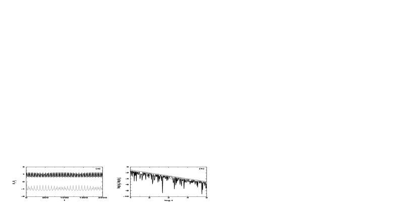
Figure 1: The time evolution of the coefficients $a_{1}$, $a_{2}$, $a_{3}$, $a_{4}$, of the initial deviation vector with $a_{1}=1$, $a_{2}=1$, $a_{3}=0$, $a_{4}=1$ (Eq. (8)). (a) $a_{1}$ (black line), $a_{2}$ (gray line). (b) $|a_{3}|$ (black line), $|a_{4}|$ (gray line) in log-log scale. The orbit of the Hamiltonian (9) used, has initial condition $x=-0.6$, $y=0$, $p_{x}=0$, $p_{y}=1.99416$. In (b) we also plot the curves $|a_{3}|=0.107\cdot t^{-0.962}$, $|a_{4}|=1.067\cdot t^{-0.995}$ that fit the data.

For different initial deviation vectors, we compute the time evolution of the coefficients $a_{1}$, $a_{2}$, $a_{3}$, $a_{4}$ of Eq. (8). We find that in all cases $a_{1}$, $a_{2}$ remain different from zero, while $a_{3}$, $a_{4}$ tend to zero. A particular example is given in Fig. 1. By fitting the data of Fig. 1b we see that $|a_{3}|$, $|a_{4}|$ $\propto t^{-1}$. From Fig. 1 we conclude that any vector will eventually fall on the “tangent space” of the torus on which the orbit evolves. This “tangent space” is produced by vectors $\widehat{f_{H}}$, $\widehat{f_{F}}$, and so any deviation vector will eventually become a linear combination of these two vectors only. As there is no particular reason for two different initial deviation vectors to end up with the same values of $a_{1}$, $a_{2}$, the SALI (1) will in general oscillate around a value different from zero. In other words the two vectors become tangent to the torus and fluctuate quasiperiodically about two different directions. This becomes evident in Fig. 2a where we plot the time evolution of the SALI for an orbit with initial conditions $x=-0.6$, $y=0$, $p_{x}=0$, $p_{y}=1.99416$ marked by a black point in the Poincaré Surface of Section (PSS) of the system seen in Fig. 2b. The initial deviation vectors used are $\overrightarrow{v_{1}}=\widehat{f_{H}}+\widehat{f_{F}}+\widehat{\nabla F}$ (the time evolution of which is given in Fig. 1) and $\overrightarrow{v_{2}}=\widehat{f_{H}}+\widehat{f_{F}}+\widehat{\nabla H}$.

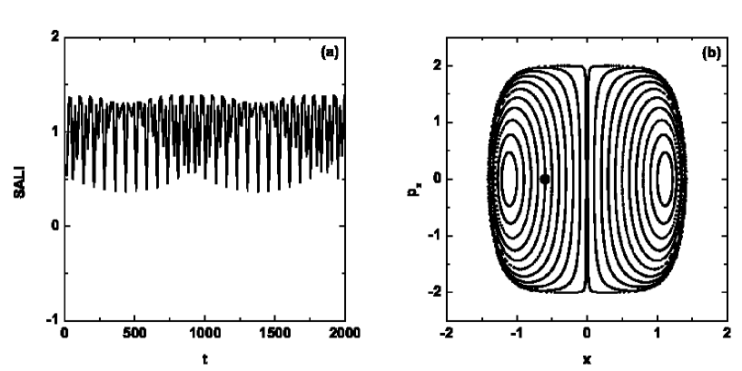
Figure 2: The time evolution of the SALI (a) for the ordered orbit marked by a black point in the PSS $y=0$ of the system (b).

3 Conclusions

In this paper we have analyzed the behavior of the SALI in regions of ordered motion, by studying the evolution of deviation vectors in the case of an integrable 2D Hamiltonian system. Using a suitable basis of 4 vectors (6) we have shown that any pair of arbitrary deviation vectors tends to the tangential space of the torus, following a $t^{-1}$ time evolution and having in general 2 different directions. This explains why for ordered orbits the SALI oscillates quasiperiodically about values that are different from zero. The same result is observed to hold in the case of ordered motion in a stability region of a non–integrable system,[2] where the presence of “islands” implies the existence of an additional approximate integral $F$, independent of the Hamiltonian. For Hamiltonian systems of more than 2 degrees of freedom we expect similar results. The only difference is that the “tangent space” is of higher dimension generated by the vectors $\widehat{f_{H}},\,\,\widehat{f_{F_{1}}},\,\,\widehat{f_{F_{2}}},\,\ldots$, with $F_{1}$, $F_{2},\,\ldots$, being the additional (approximate or not) integrals of the motion.

References

- [1] Ch. Skokos, \JLJ. Phys. A,34,2001,10029.
- [2] Ch. Skokos, Ch. Antonopoulos, T. C. Bountis and M. N. Vrahatis, in Proceedings of the 4th GRACM Congress on Computational Mechanics, ed. D. T. Tsahalis, (Univ. Patras, Patras, 2002), Vol. IV, p. 1496; in Libration Point Orbits and Applications, eds. G. Gómez, M. W. Lo and J. J. Masdemont, (World Scientific, 2003), in press, nlin.CD/0210053.
- [3] Ch. Skokos, Ch. Antonopoulos, T. C. Bountis and M. N. Vrahatis, 2003, in preparation.
- [4] M. A. Lieberman and A. J. Lichtenberg, Regular and Chaotic Dynamics (Springer Verlag, 1992).
- [5] Ch. L. Vozikis, \JLJ. Phys. A,34,2001,1513.
- [6] K. Ganesan and M. Lakshmanan, \PRA42,1990,3940.