¹Department of Mathematics and Statistics, University of Massachusetts, Amherst MA 01003-4515, USA

²Department of Interdisciplinary Studies, Faculty of Engineering, Tel Aviv University, Tel Aviv, Israel

³Department of Physics, University of Athens, Panepistimiopolis, Zografos, Athens 15784, Greece

⁴Center for Nonlinear Studies and Theoretical Division, Los Alamos National Laboratory, Los Alamos, NM 87545 USA

Abstract

We introduce domain-wall (DW) states in the bimodal discrete nonlinear Schrödinger equation, in which the modes are coupled by cross phase modulation (XPM). The results apply to an array of nonlinear optical waveguides carrying two different polarizations of light, or two different wavelengths, with anomalous intrinsic diffraction controlled by direction of the light beam, and to a string of drops of a binary Bose-Einstein condensate, trapped in an optical lattice. By means of continuation from various initial patterns taken in the anti-continuum (AC) limit, we find a number of different solutions of the DW type, for which different stability scenarios are identified. In the case of strong XPM coupling, DW configurations contain a single mode at each end of the chain. The most fundamental solution of this type is found to be always stable. Another solution, which is generated by a different AC pattern, demonstrates behavior which is unusual for nonlinear dynamical lattices: it is unstable for small values of the coupling constant $C$ (which measures the ratio of the nonlinearity and coupling lengths), and becomes stable at larger $C$. Stable bound states of DWs are also found. DW configurations generated by more sophisticated AC patterns are identified as well, but they are either completely unstable, or are stable only at small values of $C$. In the case of weak XPM, a natural DW solution is the one which contains a combination of both polarizations, with the phase difference between them $0$ and $\pi$ at the opposite ends of the lattice. This solution is unstable at all values of $C$, but the instability is very weak for large $C$, indicating stabilization as the continuum limit is approached. The stability of DWs is also verified by direct simulations, and the evolution of unstable DWs is simulated too; in particular, it is found that, in the weak-XPM system, the instability may give rise to a moving DW. The DW states can be observed experimentally in the same parameter range where discrete solitons have been found in the lattice setting.

I Introduction

Nonlinear optical fibers and waveguides and arrays composed of them furnish a unique example of a medium in which various solitary-wave patterns and their complexes can be easily observed in a real experiment, and described, with a very high accuracy, by relatively simple models, a benchmark example being the nonlinear Schrödinger equation [1]. Besides commonly known bright and dark solitons, solitary-wave structures in the form of domain walls (DWs) were also predicted in a fiber with normal group-velocity dispersion (GVD) which carries two different waves with orthogonal polarizations, circular or linear, that interact through the cross-phase modulation (XPM) induced by the Kerr nonlinearity [2, 3]. Similar structures can also be expected to exist in planar nonlinear optical waveguides [4]. DW patterns are distinguished by the property that, asymptotically, they contain a single polarization, with a switch between two of them in a localized region. In fact, solutions for the optical DWs were constructed, following the pattern of earlier known solutions of the DW type for a system of coupled Ginzburg-Landau equations that describe interactions between roll patterns with different orientations in a convection layer [5, 6].

GVD in the fiber must be normal in order to prevent the modulational instability (MI) of the DW’s uniform background fields. Nevertheless, it is known that a uniform two-component field, unlike single-component ones, may be subject to MI even in the case of normal GVD [1]. Loosely, DWs are related to the MI of the two-component uniform state the same way as the usual bright soliton is related to MI of the single-component field in the case of anomalous GVD [4].

The same model (which is presented in detail below) applies to an altogether different physical system, namely, a string of drops of a binary (two-component) Bose-Einstein condensate (BEC) trapped at minima of a periodic potential, which can be readily induced by an optical interference pattern [7]. In this connection, it is relevant to mention that stable DW configurations have been predicted in a continuous quasi-one-dimensional (cigar-shaped) binary BEC [8].

Optical DWs in nonlinear fibers have been observed in direct experiments [9], including high-repetition periodic DW trains [10]. On the other hand, recent experimental achievements in the observation of discrete spatial optical solitons in arrays of waveguides in the spatial domain [11, 12] suggest that observation of DW-like structures in waveguide arrays may be quite feasible too. Additionally, solitons of the DW type may be a new species of solitary waves in the discrete nonlinear Schrödinger (DNLS) equations, which have recently attracted a great deal of interest (for a recent review see e.g., Ref. [13]). Given that the solutions to coupled DNLS equations have been examined for a considerable while now (the first relevant results appeared about 20 years ago in [14]), it appears that DWs may be one of the few types of DNLS solitons that have not been studied yet.

An objective of the present work is to introduce this type of discrete solitons and study their stability by means of precise numerical methods. An exact formulation of the model, together with estimates of relevant physical parameters, are given in section 2. In section 3, we study in detail DWs in the case of strong XPM, which corresponds to circular polarizations. We find several different types of DWs, the simplest one being stable for all values of the inter-site coupling constant $C$ (which is the ratio of the propagation length determined by the Kerr nonlinearity to the linear-coupling length, in terms of the optical-waveguide array). DWs of a different type exhibit a rather unusual stability behavior, being stable at small values of $C$, and stable at larger $C$, i.e., in weakly and strongly coupled arrays, respectively. The existence of stable bound states of DWs is also demonstrated. Other types of DWs turn out to be either completely unstable, or stable only at small values of $C$. In section 4, we consider DWs in the model with weak XPM, which corresponds to linear polarizations. In this case, DWs are unstable. However, the instability growth rate of the simplest (fundamental) DW becomes vanishingly small for large values of $C$, so that the pattern becomes (marginally) stable in the continuum limit, $C\rightarrow\infty$. In all the cases, the predicted stability of DWs is tested in direct numerical simulations, and in those cases when DWs are expected to be unstable, the instability development is simulated too. Section 5 summarizes the paper.

II Formulation of the model

The model of an array of nonlinear optical fibers carrying fields $\phi_{n}(z)$ and $\psi_{n}(z)$, which correspond to two orthogonal polarizations of light, has the form

$$i\frac{d}{dz}\left(\psi_{n}\right) = C\left(\psi_{n+1}+\psi_{n-1}-2\psi_{n}\right)-(|\psi_{n}|^{2}+\beta|\phi_{n}|^{2})\psi_{n}\,,$$ (1)

$$i\frac{d}{dz}\left(\phi_{n}\right) = C\left(\phi_{n+1}+\phi_{n-1}-2\phi_{n}\right)-(|\phi_{n}|^{2}+\beta|\psi_{n}|^{2})\phi_{n}\,,$$ (2)

where $z$ is the propagation distance along the fiber and $n$ is the index of the lattice site. Equations (1) and (2) are written in a rescaled form, in which the constant $C$ of the linear coupling between adjacent fibers has a straightforward physical meaning: it is a ratio of the characteristic propagation length $L_{{\rm nonlin}}$ along the waveguide, determined by the Kerr nonlinearity (self-phase modulation, SPM), to the coupling length $L_{{\rm coupl}}$ determined by the linear interaction between adjacent waveguides. In the most typical experimental situation, with the power of light beams $500-1000$ W, the nonlinearity length in AlGaAs waveguides (whose nonlinearity is $500$ time stronger than that of fused silica glass) takes values $\sim 1-2$ mm, and the coupling length is $\sim 1$ mm [11, 12]. In fact, $L_{{\rm coupl}}$ may vary in broad limits, as it exponentially depends on the separation $h$ between the waveguides: for instance, $L_{{\rm coupl}}$ decreases by a factor of $1.6$ as $h$ increases from $9$ $\mu$m to $11$ $\mu$m [11]. Results displayed below (such as a width of DWs in terms of the number of lattice sites) suggest that stable DWs in optical-waveguide arrays should be observable in the same experimental setups, and in essentially the same range of the power-per-waveguide, where bright discrete solitons have been found in works [11, 12].

In Eqs. (1) and (2), the SPM coefficient is normalized to be $1$, and $\beta$ is a relative coefficient of the XPM nonlinear coupling, which is $2$ or $2/3$, in the case of linear or circular polarizations, respectively. In the latter case, we neglect, as usual, four-wave-mixing (FWM) nonlinear coupling terms [1] Strictly speaking, for the short propagation distance ($\sim 10$ mm), relevant to the recent experiments [11], it may be necessary to keep the FWM terms in the case $\beta=2/3$; we do not consider this issue in the present work because, as it will be shown below, most interesting results are found in the case $\beta=2$. We will refer to the two cases with $\beta=2/3$ and $\beta=2$ as those with the weak and strong XPM coupling, respectively. The value $\beta=2$ applies also to the case when the two modes refer not to polarizations, but rather to light signals carried by different wavelengths [1], which is another plausible realization of the present model in terms of nonlinear optics.

If the nonlinearity in the waveguides is induced by the usual self-focusing Kerr effect, and the light is launched so that its Poynting vector is oriented parallel to the array, the linear coupling between fibers (discrete diffraction) corresponds to $C<0$ in Eqs. (1) and (2). In this case, the system gives rise to two-component discrete bright solitons, which were recently studied in detail, including their generalization to the two-dimensional lattice [15]. However, a newly developed experimental technique, based on launching an oblique beam into the array [12], makes it possible to implement anomalous discrete diffraction, which corresponds to $C>0$ in Eqs. (1) and (2). In this case, bright solitons do not exist.

As it was mentioned above, the same system of Eqs. (1) and (2) may also be regarded as a normalized model of a string of binary-BEC drops trapped in an optical lattice. In this case, assuming the usual situation with the positive scattering length (i.e., repulsion between atoms), one has $C>0$, which is precisely what is necessary to generate DW solutions. Unlike the realization in terms of nonlinear optics, the value of the coefficient $\beta$ may be arbitrary (but positive). The separation between the drops is of the order of the lattice-generating light wavelength, i.e., $\sim 1$ $\mu$m. A promising candidate for the binary condensate being a mixture of ⁸⁵Rb and ⁸⁷Rb, the corresponding positive scattering lengths being $\sim 10$ nm [16]. The necessary temperature and densities of the drops can be estimated as $10^{-5}-10^{-6}$ K and $10^{11}-10^{12}$ cm^-3, which can be readily achieved by available experimental techniques

In this work, we examine discrete domain walls (DWs) in the system (1) and (2), which may be stable only if $C>0$. We will construct DW solutions, starting from the anti-continuum (AC) limit with $C=0$ [17], and using the continuation in $C$ to extend the solutions up to bifurcation points where they lose their stability, or up to the continuum limit ($C\rightarrow\infty$) when possible. Thus, we seek solutions of the form

$$\psi_{n} = \exp(i\Lambda z)u_{n}\,,$$ (3)

$$\phi_{n} = \exp(i\Lambda z)v_{n},$$ (4)

arriving at the stationary equations

$$F(u_{n},v_{n})\equiv-C\Delta_{2}u_{n}+(|u_{n}|^{2}+\beta|v_{n}|^{2})u_{n}-\Lambda u_{n} = 0,$$ (5)

$$G(u_{n},v_{n})\equiv-C\Delta_{2}v_{n}+(|v_{n}|^{2}+\beta|u_{n}|^{2})v_{n}-\Lambda v_{n} = 0.$$ (6)

Once a solution to Eqs. (5) and (6) has been found (by means of a Newton-type numerical method), we perform the linear stability analysis around it, looking for perturbed solutions as [18]

$$\psi_{n} = \exp(i\Lambda z)\left[u_{n}+\epsilon a_{n}\exp(i\omega z)+\epsilon b_{n}\exp(-i\omega^{\star}z)\right],$$ (7)

$$\phi_{n} = \exp(i\Lambda z)\left[v_{n}+\epsilon c_{n}\exp(i\omega z)+d_{n}\exp(-i\omega^{\star}z)\right]\,$$ (8)

(the asterisk stands for the complex conjugation), and solving the ensuing matrix eigenvalue problem.

III Numerical results for the strong-XPM model

In this section, we consider the model based on Eqs. (1) and (2) with $\beta=2$. We start the examination of DW structures by looking for stationary solutions in a natural form which is taken, in the AC limit, as

$$u_{n}=(...0,0,0,V_{1},1,1,1,...),\,v_{n}=(...1,1,1,V_{2},0,0,0,...)$$ (9)

[see Eqs. (3) and (4)], where $V_{1}$ and $V_{2}$ belong to one (central) site of the lattice and will be defined below. We will, in particular, consider the steady states with $\Lambda=1$ in Eqs. (3) and (4), but results will be generally true if $1$ in AC ansatz (9) is replaced by $\sqrt{\Lambda}$ for an arbitrary positive value of $\Lambda$. Notice that in the present study, we fix $\Lambda$ and vary $C$, modifying, essentially, in this way the degree of localization or equivalently the peak power. One can instead always rescale $C$ to the value $C=1$, and equivalently vary the propagation constant $\Lambda$.

Numerical calculations demonstrate that, for $\beta=2$ (which corresponds to the circular polarizations of light in the fibers), the AC pattern (9) with

$$V_{1}=1,\,V_{2}=0$$ (10)

(or vice versa) generates the most structurally robust and stable solutions. In particular, this solution was found to be stable for all values of the coupling constant $C$, up to the continuum limit $C\rightarrow\infty$. Examples of such a DW for cases of weak ($C=0.034$) and strong ($C=3.5$) inter-site coupling (recall $C$ may be realized as the ratio $L_{{\rm nonlin}}/L_{{\rm coupl}}$ in the optical-waveguide array) are shown in Fig. 1. The complete stability of DWs belonging to this branch of the solutions has also been verified by direct simulations of the full nonlinear equations (1) and (2), with initial conditions containing a small noisy component.

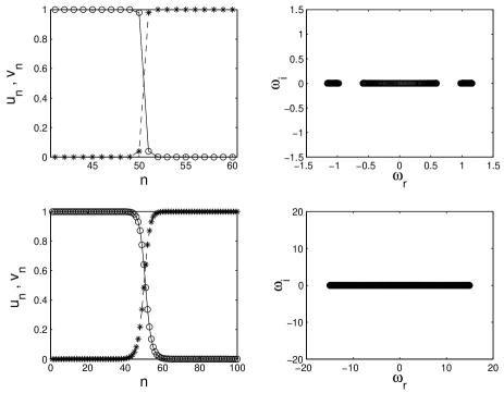
FIG. 1.: Left panels show examples of the domain-wall solutions generated, in the case $\beta=2$ and $\Lambda=1$, by the AC pattern with $u_{n}=(0,\dots,0,1,1,\dots,1)$ (the dashed line connecting the stars is as a guide to the eye) and $v_{n}=(1,\dots,1,0,0,\dots,0)$ (circles connected by the solid line). Right panels show the spectral plane ($\omega_{r},\omega_{i}$) of the corresponding stability eigenfrequencies found from the equations linearized about the stationary solution, the subscripts standing for the real and imaginary parts. The absence of eigenfrequencies with a nonzero imaginary part indicates the stability of the configuration. The top and bottom panels correspond, respectively, to $C=0.034$ (weak coupling) and $C=3.5$ (strong coupling).

The next case to consider is when

$$V_{1}=V_{2}=\sqrt{\Lambda/(1+\beta)}$$ (11)

in Eq. (9). These values imply that, in the AC limit, the central waveguide in the array carries a vectorial state, in which both polarities have equal amplitudes. The numerical investigation reveals an unusual feature of this solution branch: it is unstable for small values of $C$, starting from the AC limit ($C=0$), but becomes stable at $C=0.61$, and remains stable thereafter up to $C=\infty$. This property is opposite to the common scenario, when a sufficiently strong discreteness is responsible (through the effective potential energy barrier that it creates) for the stabilization of various solitary-wave lattice patterns (for instance, two-dimensional pulses [19] or vortices [20]) that are unstable in the continuum limit.

Solutions generated by Eq. (11) are shown, for the same values of $\beta$, $\Lambda$, and $C$ as in Fig. 1, in two upper rows of Fig. 2 (top panel). Notice the presence of an unstable (imaginary) eigenvalue pair in the panel pertaining to $C=0.034$. The imaginary part of the unstable eigenvalue is displayed, as a function of the coupling constant, in the lower panel of Fig. 2, showing the transition from instability to stability at $C\approx 0.61$.

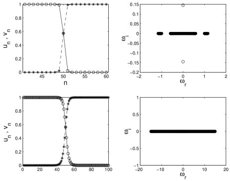
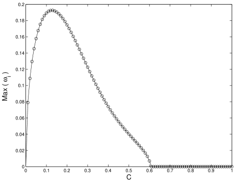
FIG. 2.: The two top rows show DW solutions and their stability eigenvalues, as generated by the AC pattern (9) at the same values of parameters as in Fig. 1, but with $V_{1}$ and $V_{2}$ chosen as in Eq. (11). The bottom panel shows the imaginary part of the most unstable eigenvalue as a function of $C$.

The predictions for the stability of these solutions were also checked against direct simulations of the full equations. In the case when the DW is predicted to be stable, it is indeed found to be completely stable (not shown here). In the case when it is expected to be unstable, the simulations show (see Fig. 3) that the unstable DW emits a packet of lattice phonons and rearranges itself so that the field in one component at one site ($n=50$) in Fig. 3) becomes equal to the field in the other component at the adjacent site ($n=51$, in Fig. 3). Comparison with the expressions (9) and (10) clearly suggests that the result of the instability development is the rearrangement of the DW into a stable one belonging to the solution branch generated by Eq. (10) in the AC limit.

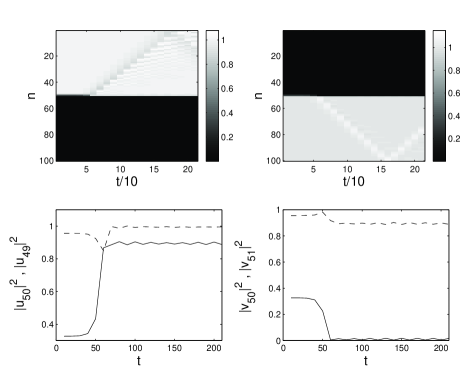
FIG. 3.: Evolution of an unstable DW configuration belonging to the solution branch generated by the AC ansatz (9) and (11) with $C=0.1$, $\beta=2$, and $\Lambda=1$. To initiate the onset of the instability, a noise with an amplitude $10^{-4}$ was added to the initial configuration. The left and right top panels display the evolution of the fields $|v_{n}|$ and $|u_{n}|$, while the bottom panels show the evolution of the fields at the sites $n=50$ (solid curve) and $n=49$ (dashed curve) for $u$, and $n=50$ (solid curve) and $n=51$ (dashed) for $v$.

A solution generated by the AC pattern (9) with $V_{1}=V_{2}=0$ (i.e., with both field components equal to zero at the central lattice site in the AC limit) was also examined. Unlike the solution branches considered above, this one does not reach the continuum limit. Instead, it terminates at $C=0.15143$ through a turning-point bifurcation. This is obvious in Fig. 4, which displays the $L^{2}$ norm of one component of the solution (the other component behaves similarly),

$$P\equiv\left(\sum_{-\infty}^{+\infty}u_{n}^{2}\right)^{1/2}\,,$$ (12)

vs. the coupling constant $C$ (note that $P$ is finite due to the finiteness of the computational domain). The dependence $P(C)$, shown in Fig. 4, is not a completely invariant characteristic, as values of $P$ depend on the size of the domain. However, the turning-point structure is invariant.

In the lower panel of Fig. 4, the present solution and its linear stability eigenvalues are shown for three different values of $C$ ($C=0.06$, $C=0.11$, and $C=0.15143$ in the in the top, middle, and bottom subplots). As is seen from this part of the figure, the first solution is stable, while the latter two are not. The solutions of the present type are stable for $C<0.0725$, and the spectrum of their linear-stability eigenvalues contains two continuous bands. As $C$ increases, two pairs of eigenvalues bifurcate from the outer band and move towards the inner one. Their first collision with the inner band occurs at $C\approx 0.0725$, and the second collision takes place at $C\approx 0.08$. Each collision generates an instability-bearing quartet of eigenvalues, manifesting the so-called Hamiltonian Hopf bifurcation [21]. Subsequently (for larger $C$), the two quartets move towards the imaginary eigenvalue axis. Very close to the turning point, the collision of the first quartet with the axis induces a symmetry breaking, which results in one pair of eigenvalues moving towards the origin, while another pair moves upwards along the imaginary axis. Finally, as a result of the collapse of the lower imaginary pair onto the origin of the spectral plane, the turning-point bifurcation occurs and the branch terminates, as is shown in the upper panel of Fig. 4.

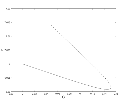
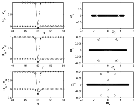
FIG. 4.: The upper panel demonstrates the result of continuation of the branch with $V_{1}=V_{2}=0$ from the AC limit up to the turning point ($C\approx 0.15143$) – the solid curve – and back – the dashed one. To this end, the $L^{2}$ norm $P$ (see Eq. (12)) of one component (the other behaves similarly) of the solution is shown as a function of the coupling constant $C$. The lower panel shows solutions at three points along the solid line in the upper panel. In particular, the stable solution for $C=0.06$ (its spatial profile and stability) is shown in the top subplot, and solutions for $C\approx 0.11$ and $C\approx 0.15142$ (the latter one being very close to the turning point) are displayed in the middle and bottom subplots.

Direct simulations again show that the solutions which are stable according to the linearization are indeed stable in full simulations. An example of direct simulations of the unstable solution belonging to this branch is given in Fig. (5). As is seen, the instability does set in, but its growth is extremely slow.

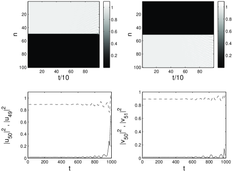
FIG. 5.: The evolution of a weakly unstable solution generated, in the AC limit, by the ansatz (9) with $V_{1}=V_{2}=0$, for $C=0.1$, $\beta=2$, $\Lambda=1$. The development of the instability is initiated by adding noise with an initial amplitude $10^{-3}$. The meaning of the panels is the same as in Fig. 3.

We also considered the situation with the zero-field state occupying, in the AC limit, two (or more) lattice sites. The resulting scenario turns out to be similar to that demonstrated above for the patterns generated by the AC limit (9) with $V_{1}=V_{2}=0$: the solution is stable at very small $C$, then becomes unstable due to the bifurcation of four (instead of two in the previous case) pairs of eigenvalues from the outer band and their collision with the inner band (not shown here). Finally, the branch terminates at a turning point at $C\approx 0.17$, similarly to what was shown in Fig. 4. Note that this turning point is found at a larger value of $C$ than in Fig. 4. We continued the analysis, starting with several empty (zero-field) sites in the center of the pattern at $C=0$, which produced quite a similar picture, an unexpected feature being that the value of $C$ at the turning point increases with the increase of the number of the initially empty sites.

Contrary to what was described above for the case of one or several empty sites, in the case when the initial pattern has two sites occupied by the vectorial state (11), the solution behaves quite differently from its counterpart in the case when only one site was initially occupied by the vectorial state. In fact, not only does the branch terminate - in this case, at $C\approx 0.1085$ (the solution found at the turning point and its stability eigenvalues are shown in Fig. 6) - but it is also found to be always unstable: for every value of $C$ starting from the AC limit $C=0$, there are two imaginary eigenvalue pairs. The branch terminates when one of them passes through the origin.

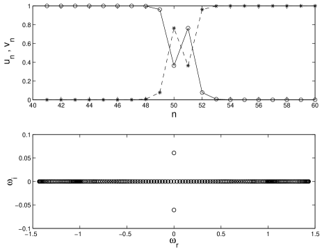
FIG. 6.: The solution generated, in the AC limit, by the pattern with two sites occupied by the vectorial state (11) is shown exactly at the turning point of $C\approx 0.1085$, along with its stability eigenvalues. This solution branch is always unstable, as discussed in the text.

An example of directly simulated evolution of an unstable DW of this type is shown in Fig. 7. In this case, the instability development is essentially faster than in the case shown in Fig. 3, and, as a result, a stable DW appears.

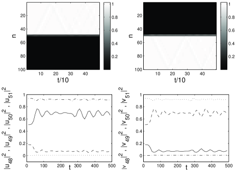
FIG. 7.: The evolution of an unstable solution generated, in the AC limit, by the ansatz (9) with two sites occupied by the vectorial state (11), for $C=0.1$, $\beta=2$, $\Lambda=1$. The development of the instability is initiated by adding noise with an initial amplitude $10^{-4}$. The meaning of the panels is the same as in Fig. 3, the bottom ones showing (absolute value of) the field evolution at the points $n=48$ (dash-dotted lines), $n=49$ (dashed lines), $n=50$ (solid lines), and $n=51$ (dotted lines) for $u$ (bottom left) and $v$ (bottom right) as a function of time $t$.

Furthermore, stable DW solutions found above, such as the ones generated by the AC-limit pattern (9) with $V_{1}$ and $V_{2}$ chosen as per Eqs. (10) or (11), can form stable complexes (higher-order DWs). Obviously, the complex must contain an odd number of fundamental DWs. An example is shown in Fig. 8 for $C=0.15$. Direct simulations confirm that these complexes are completely stable.

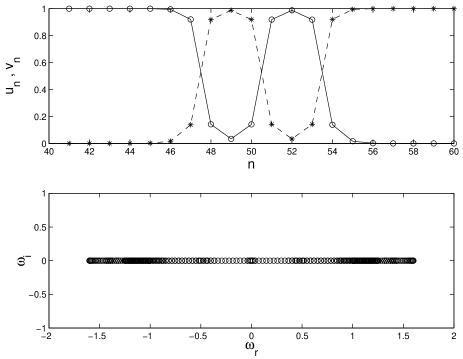
FIG. 8.: An example of a stable complex consisting of three domain walls for $C=0.15$. Shown are the solution’s spatial profile (top panel) and stability eigenvalues (in the bottom panel).

Recall that, if the underlying system of Eqs. (1) and (2) is applied to the string of BEC drops, the value of $\beta$, which is determined by the values of the cross-scattering length, is arbitrary. In the case $\beta>1$, the results are quite similar to those described in detail above for $\beta=2$. For $\beta<1$, the results are very different, as is described in the next section.

IV The weak-XPM model

The underlying pattern (9), used to construct all the DW states considered above, was suggested by solutions found (in the temporal, rather than spatial, domain) in the continuum model of the single nonlinear optical fiber [3, 4] or cigar-shaped BEC [8]. Solutions of this type in the continuum model exist only in the case of sufficiently strong XPM, namely, for $\beta>1$.

Unlike the continuum model, in the discrete system (1), (2) DW patterns of the type (9) can also be found for $\beta<1$ (weak XPM coupling), including the case $\beta=2/3$, which is specially relevant for the applications to nonlinear optics. However, in this case properties of the DW solutions are drastically different from those described above for $\beta=2$.

For $\beta=2/3$, all solutions of the DW type were observed to become staggered when continued from the AC limit (i.e., the phase difference between the fields at adjacent sites of the lattice tends to be $\pi$, rather than $0$). As a result, the outer continuous band of the stability eigenvalues has the Krein signature [22] opposite to that of the inner band, and as soon as the bands collide (which happens at $C\approx 0.011$, i.e., still in the case of very weak coupling), numerous quartets of complex eigenvalues arise. An example, corresponding to the solution generated by the AC pattern (9) with the central site occupied by the vectorial state (11) (with $\beta=2/3$) is displayed in Fig. 9. Similar results were obtained for the solution branches generated by the pattern (9) with $V_{1}=1$ and $V_{2}=0$ (also with $\beta=2/3$). Thus, discrete DW solutions of this type may exist in the weak-XPM case, unlike the continuum limit, but they are stable only at very small values of the coupling constant. These conclusions, concerning the existence and (in)stability of the DW patterns for the weak-XPM case, are corroborated by direct simulations; however, the instability is extremely slow, therefore it is not shown here.

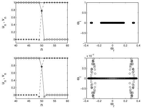
FIG. 9.: The DW solution and the corresponding stability eigenvalues prior to the onset of the oscillatory instabilities (for $C=0.004$), and after the onset (for $C=0.017$), in the case $\beta=2/3$ and $\Lambda=1$.

In the regime of weak XPM, another type of DW solutions is suggested by analogy to the findings of Ref. [3] for the continuum version of the model. This type of solution exists only for the weak-XPM case ($\beta<1$) in the continuum model, and, quite naturally, turns out to be primarily relevant in the same case in the discrete model. In the continuum limit, this solution is

$$u(x)=\sqrt{\Lambda}\cos(\chi),\,v(x)=\sqrt{\Lambda}\sin(\chi),$$ (13)

where $\Lambda$ is the same as in Eqs. (3) and (4), and, in the first approximation (which corresponds to a broad DW),

$$\chi(x)=\frac{\pi}{4}-\tan^{-1}\left[\exp(-s\sqrt{\epsilon\Lambda}x)\right],\,\epsilon\equiv 1-\beta.$$ (14)

The corresponding AC limit of such solutions is (for $\Lambda=1$)

$$u_{n}=(1/\sqrt{2},\dots,1/\sqrt{2},1/\sqrt{2},\dots,1/\sqrt{2}),\,v_{n}=(-1/\sqrt{2},\dots,-1/\sqrt{2},1/\sqrt{2},\dots,1/\sqrt{2}).$$ (15)

Starting from Eq. (15), the solution was extended all the way from $C=0$ to the continuum limit, which shows that the solution exists for all values of $C$. The upper panel of Fig. 10 shows two examples of this solution, for $C=0.034$ and $C=3$. The lower panel of the figure clearly shows that this DW state is unstable at all values of $C$, but gets stabilized in the continuum limit, $C\rightarrow\infty$. For instance, for $C=3$ the growth rate of the relevant instability is already extremely small, $\sim 10^{-6}$, hence this state may seem a practically stable one in the discrete case too, provided that the coupling constant is large enough.

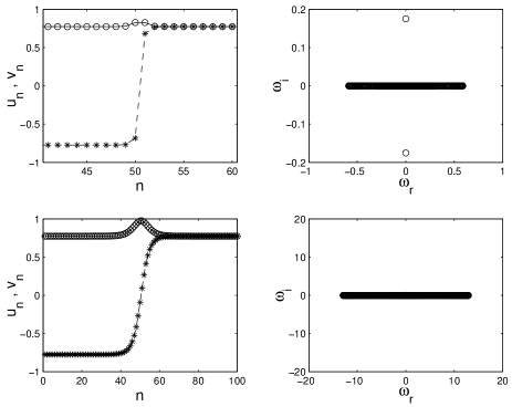
FIG. 10.: The upper panel shows the discrete counterpart of the continuum-model solutions (13) for $C=0.034$ (top panel) and $C=3$ (bottom panel). The stability eigenvalues for both configurations are shown in the respective right subplots. The lower panel shows the $L^{2}$ norm of the two branches (the solid and dashed lines correspond to the norms of the fields $u_{n}$ and $v_{n}$, respectively), and the imaginary part of the most unstable eigenvalue vs. $C$.

These predictions for the DW patterns generated by the ansatz (15) were verified in direct simulations of the full nonlinear system with $\beta=2/3$. Figure 11 shows the development of the relatively strong instability in the case $C=0.1$. A remarkable result, which makes this case drastically different from those considered above, is that the instability transforms the quiescent DW into a moving one, which is accompanied by emission of quasi-linear lattice waves.

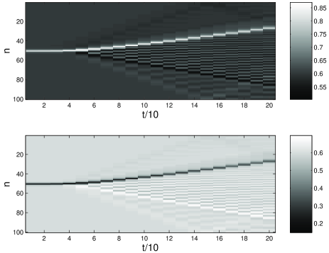
FIG. 11.: The (norm contour plot of the) development of the instability of the DW solution generated by the ansatz (13) in the AC limit in the weak-XPM case, $\beta=2/3$, and $C=0.1$, $\Lambda=1$. The instability is initiated by adding noise with an initial amplitude $10^{-4}$.

It has also been verified that, in full accordance with the prediction of the linear-stability analysis, the formally unstable DWs of the present type seems to be virtually stable ones. A typical example of that is displayed in Fig. 12.

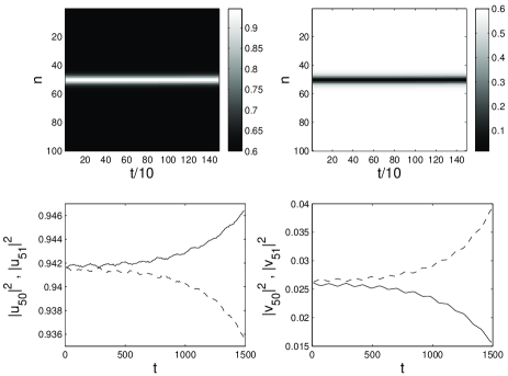
FIG. 12.: The instability of the DW solution generated by the ansatz (13) in the AC limit in the weak-XPM case, $\beta=2/3$, and $C=1$, $\Lambda=1$. The instability is initiated by adding noise with an initial amplitude $10^{-4}$. The upper panels show the evolution of the fields $|u_{n}|$ and $|v_{n}|$, while the lower ones specially show the evolution of the fields at the sites $n=50$ and $n=51$, by means of the solid and dashed curves, respectively. As it is obvious from the lower panels, the growth of the instability is extremely slow.

Even though the continuum-limit analytical expressions (13) - (14) for these solutions are only valid for $\beta<1$, one can seek for similar solutions in the discrete strong-XPM system, with $\beta=2$. The same way as solutions of the type (9) can exist in the discrete system with $\beta=2/3$, despite the fact that they do not exist in the continuum limit for the weak-XPM case (see above), the solutions of the type (13) - (14) have a chance to exist in the discrete strong-XPM model. We have found that such solutions indeed exist for very small values of $C$, but they exhibit very strong instabilities, with a part of the imaginary eigenvalue axis being populated by the continuous spectrum. In Fig. 13, a solution of this type for $\beta=2$ and $C=0.12$ is compared with a “natural” one existing at $\beta=2/3$ and $C=0.2$.

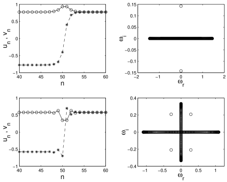
FIG. 13.: The solution of the type (13)-(14) is shown for $C=0.2$ in the top panel, along with its stability eigenvalues. For comparison, the bottom panel shows a solution of the same type for $\beta=2$, $C=0.12$. Notice the continuous-spectrum-induced instabilities in the latter case.

The nonlinear evolution of this strong instability was directly simulated, showing a quick transition to a state of “lattice turbulence”, see Fig. 14. Thus, the lattice admits the existence of the “unnatural” solutions in both strong- and weak-XPM cases, but it never allows them to persist ad infinitum.

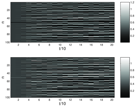
FIG. 14.: The instability of the DW solution generated by the ansatz (13 in the AC limit in the strong-XPM case, $\beta=2$, and $C=0.1$, $\Lambda=1$. The instability is initiated by adding noise with an initial amplitude $10^{-4}$, leading very rapidly to lattice turbulence. The panels show the time evolution of the (contours of the squares of the) fields $|u_{n}|$ and $|v_{n}|$.

V Conclusions

In this work we have studied, by means of numerical methods, the structure and stability of domain-wall (DW) solutions in the system of two discrete nonlinear Schrödinger equations with the coupling of the cross phase modulation (XPM) type. The consideration of this problem is suggested by the analogy with known DW solutions in a standard model of a nonlinear optical fiber carrying two polarizations of light or two different wavelengths, as well as in the quasi-one-dimensional binary Bose-Einstein condensate (BEC). The results directly apply to an array of fibers of this type, with the anomalous intrinsic diffraction controlled by the direction of the light beam, or to a string of BEC drops trapped in an optical-lattice potential; in the latter case, the generic case with the positive scattering lengths is that which may give rise to DW patterns.

Using Newton-type methods and continuation from various initial patterns, starting from the anti-continuum (AC) limit, we have found a number of different stationary solutions of the DW type (while the continuum model admits a single type of the DW solution). Different stability scenarios and transitions to instability were identified for these solutions. In the case of strong XPM coupling, corresponding to two circular polarizations or two different wavelengths in the optical-waveguide array, natural DW configurations contain only one polarization at each end of the chain. The most fundamental solution of this type, generated by the simplest AC pattern, has been found to be always stable. Another solution, generated by the AC pattern that includes a vectorial state in the central site of the lattice, generates a behavior which is unusual for nonlinear dynamical lattices: it is unstable for small values of the coupling constant $C$ (which is the ratio of the nonlinear propagation length to the coupling length in the waveguide array), acquiring stability and remaining stable at larger values of $C$. Stable bound states formed by stable DWs were also found. A number of DW configurations generated by more sophisticated AC patterns were obtained, but they were either found to be completely unstable, or to be stable only at very small values of $C$.

In the case of weak XPM, which corresponds to linear polarizations in optics, the solutions become staggered and are subject to oscillatory instabilities. In this case, a more natural DW solution is the one with a combination of both polarizations, with the phase difference between them being $0$ and $\pi$ at the opposite ends of the lattice. This solution is unstable at all values of $C$, but the instability is very weak for large values of $C$, corresponding to stabilization in the continuum limit.

The robustness of all the patterns that were predicted to be stable in direct simulations was corroborated in direct simulations of the full nonlinear system. The evolution of unstable patterns was simulated too. In some cases, this instability is extremely weak; in other cases, a stronger instability leads to rapid rearrangement of the unstable DW into a stable one, including the possibility of generation of a moving DW in the weak-XPM model; a very strong instability may even induce “lattice turbulence”.

Estimates of physical parameters necessary for the formation of DWs in the optical-waveguide array and BEC string were given too. In particular, discrete optical DWs are expected to be found in the same region of parameters were bright discrete solitons have been already observed.

The consideration of DW patterns in dynamical lattices can be continued in several directions. A topic of direct interest concerns the mobility of DWs across the lattice. Note, in particular, that a mechanical twist applied to an optical fiber may give rise to a driving force acting on DWs in it [3], which can support the motion. On the other hand, a weak symmetry-breaking deformation of the waveguides will induce linear mixing between the two orthogonal polarizations, which will drastically affect the DWs. Another interesting problem is the interaction between DWs (in Ref. [3], it was shown that a bound state of two DWs with opposite polarities is possible in a nonlinear optical fiber in the presence of the twist). These issues will be considered elsewhere.

REFERENCES

- [1] G.P. Agrawal, Applications of Nonlinear Fiber Optics (Academic Press: San Diego, 2001).
- [2] S. Wabnitz and B. Daino, Phys. Lett. A 182, 289 (1993).
- [3] B.A. Malomed, Phys. Rev. E 50, 1565 (1994).
- [4] M. Haelterman and A. Sheppard, Phys. Lett. A 185, 265 (1994).
- [5] B.A. Malomed, A.A. Nepomnyashchy, and M.I. Tribelsky, Phys. Rev. A 42, 7244 (1990).
- [6] A. Hari and A.A. Nepomnyashchy, Phys. Rev. E 50, 1661 (1994); Phys. Rev. E 61, 4835 (2000).
- [7] D.-I. Choi and Q. Niu, Phys. Rev. Lett. 82, 2022 (1999); A.V. Taichenachev, A.M. Tumaikin, V.I. Yudin, J. Opt. B: Quant. Semicl. 1, 557 (1999); P. Pedri, L. Pitaevskii, S. Stringari, C. Fort, S. Burger, F.S. Cataliotti, P. Maddaloni, F. Minardi, and M. Inguscio, Phys. Rev. Lett. 87, 220401 (2001); H. Pu, W. Zhang, and P. Meystre, Phys. Rev. Lett. 87, 140405 (2001).
- [8] M. Trippenbach, K. Goral, K. Rzazewski, B. Malomed, and Y.B. Band, J. Phys. B: Atom. Mol. Opt. 33, 4017 (2000); S. Coen and M. Haelterman, Phys. Rev. Lett. 87, 140401 (2001).
- [9] S. Pitois, G. Millot, and S. Wabnitz, Phys. Rev. Lett. 81, 1409 (1998).
- [10] J.M. Dudley, F. Gutty, S. Pitois, and G. Millot, IEEE J. Quant. Electr. 17, 587 (2001).
- [11] H.S. Eisenberg, Y. Silberberg, R. Morandotti, A.R. Boyd, and J.S. Aitchison, Phys. Rev. Lett. 81, 3383 (1998); R. Morandotti, U. Peschel, J.S. Aitchison, H.S. Eisenberg, and Y. Silberberg, Phys. Rev. Lett. 83, 2726 (1999).
- [12] H.S. Eisenberg, Y. Silberberg, R. Morandotti, and J.S. Aitchison, Phys. Rev. Lett. 85, 1863 (2000); R. Morandotti, H.S. Eisenberg, Y. Silberberg, M. Sorel, and J.S. Aitchison, Phys. Rev. Lett. 86, 3296 (2001).
- [13] P.G. Kevrekidis, K.Ø. Rasmussen, and A.R. Bishop, Int. J. Mod. Phys. B 15, 2833 (2001).
- [14] J.C. Eilbeck, P.S. Lomdahl and A.C. Scott, Phys. Rev. B 30, 4703 (1984).
- [15] G.T. Von Nessi, Study of Discrete Breathers in a Two-Component DNLS system in Los Alamos Summer School Proceedings (LA-UR-01-4922); J. Hudock, P.G. Kevrekidis, B.A. Malomed and D.N. Christodoulides (unpublished).
- [16] J.P. Burke, Jr., J.L. Bohn, B.D. Esry, and H. Greene, Phys. Rev. Lett. 80, 2097 (1998).
- [17] R.S. MacKay and S. Aubry, Nonlinearity 7, 1623 (1994).
- [18] see e.g., J.C. Eilbeck, P.S. Lomdahl, and A.C. Scott, Physica 16D, 318 (1985); J. Carr and J.C. Eilbeck, Phys. Lett. A 109, 201 (1985).
- [19] P.G. Kevrekidis, K.Ø. Rasmussen, and A.R. Bishop, Phys. Rev. E 61, 2006 (2000).
- [20] B.A. Malomed and P.G. Kevrekidis, Phys. Rev. E 64, 026601 (2001).
- [21] J.-C. van der Meer, Nonlinearity 3, 1041 (1990); I.V. Barashenkov, D.E. Pelinovsky and E.V. Zemlyanaya, Phys. Rev. Lett. 80, 5117 (1998); A. De Rossi, C. Conti and S. Trillo, Phys. Rev. Lett. 81, 85 (1998).
- [22] S. Aubry, Physica 103D, 201 (1997).