Semiclassical Study on Tunneling Processes via Complex-Domain Chaos

Abstract

We investigate the semiclassical mechanism of tunneling process in non-integrable systems. The significant role of complex-phase-space chaos in the description of the tunneling process is elucidated by studying a simple scattering map model. Behaviors of tunneling orbits are encoded into symbolic sequences based on the structure of complex homoclinic tanglement. By means of the symbolic coding, the phase space itineraries of tunneling orbits are related with the amounts of imaginary parts of actions gained by the orbits, so that the systematic search of significant tunneling orbits becomes possible.

I Introduction

Tunneling is one of the most typical and important phenomena in quantum physics, and for the past several years there is growing interest in natures of tunneling processes inherent in multi-dimensions. Quantum properties in multi-dimensional systems have been investigated extensively in terms of classical dynamical concepts in the field of quantum chaos Gutzwiller , where the role of chaos, which is a generic property in multi-dimensional classical systems, has been elucidated. It was found that tunneling properties are also strongly influenced by whether underlying classical dynamics is chaotic or not Wilkinson ; Lin ; Bohigas1 ; ShudoIkeda1 ; Frischat ; Creagh ; CreaghTunnelReview , though tunneling process has no classical counterpart.

Tunneling occurs typically between classical invariant components separated in phase space, such as between regular tori or chaotic seas. On one hand, mechanism of tunneling between distinct tori separated by chaotic seas has been studied in the context of chaos-assisted tunneling Bohigas1 , and its semiquantum analysis has been done, in which the diffusion process in the chaotic sea accompanied with tunneling paths from and into the tori around the boundaries of the sea is considered to dominate the tunneling transport Frischat . Experiments have also been performed by measuring microwave spectra in the superconducting cavity Dembowski , and measuring momentum distributions of cold atoms in an amplitude-modulated standing wave of light Hensinger_et_al ; Steck_et_al .

On the other hand, tunneling between two chaotic seas separated by an energy barrier has been studied by symmetric double wells Creagh . It has been shown that the spectra of tunnel splittings are reproduced by the orbits which consist of instanton process under the barrier and homoclinic exploration in each chaotic well.

Generic aspects of the link between tunneling process and real domain process in non-integrable systems have been examined in oscillatory scattering systems TakahashiYoshimotoIkeda . They made an energy domain analysis for a model with continuous flow, while in the present study we make a time domain one for a scattering map. The semiclassical interpretation of complicated wave functions has been given in terms of oscillations of the stable manifold and an inherent property in flow systems, the divergent behavior of movable singularities of classical solutions on the complex time plane.

In near-integrable regime, the role of resonances has been elucidated in the tunneling transport between symmetric tori, by means of classical and quantum perturbation theories Brodier .

In any case, if one wants to know mechanism of tunneling in chaotic systems by relating it with the underlying classical structure, the use of complex orbits is inevitable Miller , since tunneling is a purely quantum mechanical process and is not describable in terms of real classical dynamics. Full account of such a process should, therefore, be given by complex classical dynamics. An attempt to make a full complex semiclassical analysis using the complex classical dynamics has been performed to understand which kinds of complex trajectories describe characteristic features of tunneling in the presence of chaos, and how the complex classical dynamics actually enters into real physical process ShudoIkeda1 ; OnishiShudoIkedaTakahashi1 ; Adachi .

In Ref. ShudoIkeda1 , it was found that the initial values of orbits which play a semiclassically primary role form chain-like structures on an initial-value plane. A phenomenology describing tunneling in the presence of chaos based on such structures has been developed.

In Ref. OnishiShudoIkedaTakahashi1 , the first evidence has been reported which demonstrates the crucial role of complex-phase-space chaos in the description of tunneling process by analyzing a simple scattering map. Also in this case, it was found that initial values of orbits playing a semiclassically primary role form chain-like structures on the initial-value plane.

Very recently, the chain-like structures are shown to be closely related to the Julia set in complex dynamical systems ShudoIshiiIkeda . The Julia set is defined as the boundary between the orbits which diverge to infinity and those which are bound for an indefinite time. Chaos occurs only on the Julia set Milnor . In Ref. ShudoIshiiIkeda , it was proven that a class of orbits which potentially contribute to a semiclassical wave function is identified as the Julia set. It was also shown that the transitivity of dynamics and high density of trajectories on the Julia set characterize chaotic tunneling.

However, there still remains a problem in complex semiclassical descriptions. Significant tunneling orbits are always characterized by a property that the amount of imaginary parts of classical actions gained by the orbits are minimal among the whole candidates. It is, however, difficult to find such significant orbits out of the candidates, because an exponential increase of the number of candidates with time preventing us from evaluating the amount of imaginary part of action for every candidate.

To solve this problem, in this paper, we investigate the structure of complex phase space for a scattering map model, and relate the structure to the amounts of imaginary parts of actions gained by tunneling orbits. Our main idea is to relate the symbolic dynamics of a homoclinic tanglement emerging in complex domain to the behavior of tunneling orbits. It enables us to estimate the amounts of imaginary parts of actions gained by the tunneling orbits from symbolic sequences.

The organization of the paper is as follows. In Sec. II, the symbolic description of tunneling orbits is developed. This description requires an effective symbolic dynamics constructed on a complex homoclinic tanglement. In that section, we emphasize the importance of the application of the symbolic dynamics to tunneling, and the details of how we construct the symbolic dynamics itself is deferred to Sec. III. So it should be noted that in Sec. II we use the result in Sec. III without any technical details.

More precisely, in Sec. II, the tunneling process is investigated by the time-domain approach of complex semiclassical method. We introduce a scattering map which would be the simplest possible map modeling the energy barrier tunneling in more than one degree of freedom. Though real-domain chaos is absent in this model, it is shown that tunneling wave functions exhibit the features which have been observed in the systems creating real-domain chaos, such as the existence of plateaus and cliffs in the tunneling amplitudes and erratic oscillations on the plateaus.

It is elucidated that such tunneling features originate from chaotic classical dynamics in the complex domain, in other words, the emergence of homoclinic tanglement in the complex domain. The symbolic description of the tanglement is introduced, and is applied to the symbolic encoding of the behaviors exhibited by semiclassical candidate orbits. The amounts of imaginary parts of actions gained by the orbits are estimated in terms of symbolic sequences assigned to the orbits. Significant tunneling orbits are selected according to the estimation.

Finally, tunneling wave functions are reproduced in terms of such significant orbits, and the characteristic features appearing in tunneling amplitudes are explained by the interference among such significant orbits.

In Sec. III, the technical aspects which are skipped in Sec. II are described in full details. We first investigate the construction of a partition of complex phase space. The homoclinic points are encoded into symbolic sequences by means of the partition. Then some numerical observations are presented which relates the symbolic sequences and the locations of homoclinic points in phase space. On the basis of the observations, we study the relation between the symbolic sequences and the amounts of imaginary parts of actions gained by homoclinic orbits. As a result, a symbolic formula for the estimation of imaginary parts of actions is derived.

In Sec. IV, we first conclude our present study, then discuss the role of complex-domain chaos played in semiclassical descriptions of tunneling in non-integrable systems. It is suggested that the complex-domain chaos plays an important role in a wide range of tunneling phenomena of non-integrable systems. Finally some future problems are presented.

II Semiclassical Study on Tunneling Process via Complex-Domain Chaos

II.1 Tunneling in a Simple Scattering System

We introduce a simple scattering map model which will be used in our study. The Hamiltonian of our model is given as follows:

$${\cal H}(q,p,t) = T(p)+V(q)\sum_{n=-\infty}^{+\infty}\delta(t-n),$$ (1a)

$$T(p) = p^{2}/2,$$ (1b)

$$V(q) = k\exp(-\gamma q^{2}),$$ (1c)

where $k$ and $\gamma$ are some parameters with positive values, and the height and width of an energy barrier are given by $k$ and $1/\sqrt{2\gamma}$ respectively. A set of classical equations of motion is given as

$$\left(q_{j+1},p_{j+1}\right) = f\left(q_{j},p_{j}\right),$$ (2a)

$$f:{\mathbb{R}}^{2}\rightarrow{\mathbb{R}}^{2}\,\,\,\big{|}\,\,\,\left(q,p\right) \mapsto \left(q+T^{\prime}(p),p-V^{\prime}(q+p)\right),\ \ \$$ (2b)

where $j$ denotes a time step with an integer value, and the prime denotes a differentiation with respect to the corresponding argument. ${\mathbb{R}}^{2}$ denotes real phase space.

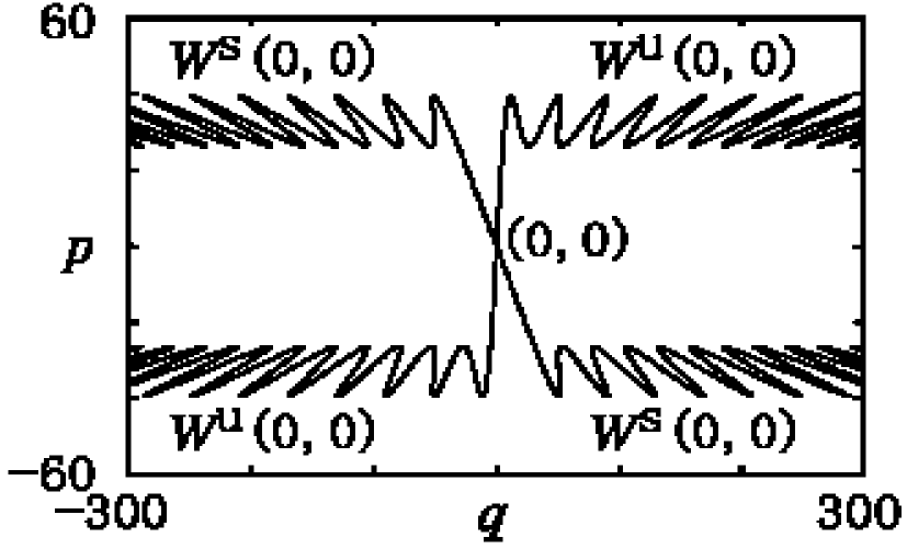
Figure 1: Real-domain stable and unstable manifolds of the unstable fixed point located at the origin.

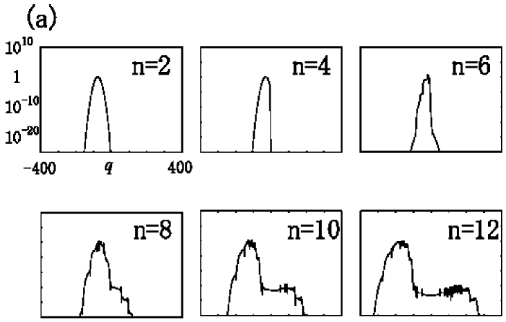
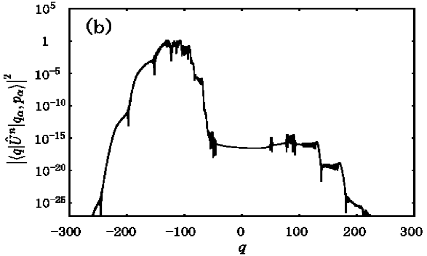
Figure 2: (a) Squared amplitudes of wave functions, $\bigl{|}\langle q|\hat{U}^{n}|q_{\alpha},p_{\alpha}\rangle\bigr{|}^{2}$, evaluated quantum-mechanically for $n=2$ to 12 in every 2 time steps ($\hbar\!=\!1,$ $\sigma\!=\!10,$ $k\!=\!500,\gamma\!=\!0.005,$ $q_{\alpha}\!=\!-123,$ $p_{\alpha}\!=\!23$). The incident wave packet is set in the asymptotic region in the side of $q<0$. In the lower figures, the center of mass has been already reflected by the potential barrier located around the origin, and those amplitudes observed in the transmitted region represent tunneling effect. (b) The enlarged figure at $n=10$.

Fig. 1 shows the stable and unstable manifolds of a fixed point located at the origin $(0,0)$. These manifolds are denoted as ${\cal W}^{s}(0,0)$ and ${\cal W}^{u}(0,0)$ respectively. We should note that the map does not create chaos in real phase space, in contrast to the maps defined in bounded phase space such as the standard map LichtenbergLieberman . One can recognize this fact in several ways: for example, the map has only single periodic orbit, $(q,p)=(0,0)$. It means that the topological entropy of the system is null. The other way is that ${\cal W}^{s}(0,0)$ and ${\cal W}^{u}(0,0)$ oscillate without creating homoclinic intersections. Any classical manifold initially put on the real phase space is stretched but not folded completely, and it goes away to infinity along ${\cal W}^{u}(0,0)$.

The quantum mechanical propagation for a single time step is given by the unitary operator:

$$\hat{U}=\exp\left[-\frac{\rm i}{\hbar}V(\hat{q})\right]\exp\left[-\frac{\rm i}{\hbar}T(\hat{p})\right],$$ (3)

where $\hat{q}$ and $\hat{p}$ denote the quantum operators corresponding to $q$ and $p$ respectively, which satisfy the uncertainty relation $[\hat{q},\hat{p}]\,=\,{\rm i}\hbar$. A quantum incident wave packet is put in an asymptotic region. The initial wave packet is given by a coherent state of the form:

$$\langle q|q_{\alpha},p_{\alpha}\rangle=\frac{1}{(\pi\hbar\sigma^{2})^{1/4}}\exp\left[-\frac{(q-q_{\alpha})^{2}}{2\hbar\sigma^{2}}-{\rm i}\frac{p_{\alpha}(q_{\alpha}-2q)}{2\hbar}\right],$$ (4)

where $\sigma$ is a positive parameter and the width of the wave packet in the $q$ direction is given by $\sqrt{\hbar}\sigma$. $q_{\alpha}$ and $p_{\alpha}$ are the position and momentum of the center of mass, respectively. The initial kinetic energy is set to be far less than the potential barrier.

Fig. 2 shows the iteration of the quantum wavepacket. Several features are observed such as amplitude crossovers, the existence of plateaus and cliffs, and erratic oscillations on the plateaus. The same features have been reported in the case of dynamical tunneling in mixed phase space ShudoIkeda1 . These are called the “plateau-cliff structure”, which has been confirmed in several systems as a typical structure of tunneling wave functions in the presence of real-domain chaos ShudoIkeda1 . However, as seen in our system, the existence of the plateau-cliff structure does not always need chaotic dynamics in real phase space. So, the features of wave functions observed here would be beyond our intuitive expectation based on the real classical dynamics. This strongly motivates the use of complex trajectories and complex semiclassical analysis to describe the features.

II.2 Formulation of Semiclassical Analysis

In the complex semiclassical analysis of our system, it is convenient to define a pair of canonical variables $(Q,P)$ by

$$Q = \frac{\sigma}{\sqrt{2}{\rm i}}(p+{\rm i}q\sigma^{-2}),$$ (5a)

$$P = \frac{\sigma}{\sqrt{2}}\,\,(p-{\rm i}q\sigma^{-2}),$$ (5b)

and some notations by

$$(Q_{0},P_{0}) = \left(Q(q_{0},p_{0}),P(q_{0},p_{0})\right),$$ (6a)

$$(Q_{\alpha},P_{\alpha}) = \left(Q(q_{\alpha},p_{\alpha}),P(q_{\alpha},p_{\alpha})\right),$$ (6b)

where $(q_{0},p_{0})$ and $(q_{\alpha},p_{\alpha})$ denote respectively the initial value of the classical map $f$, and the value specifying the center of the wave packet (4).

The wave function $\langle q|U^{n}|q_{\alpha},p_{\alpha}\rangle$ is represented by an n-fold multiple integral:

$${\cal A}_{n}\int dq_{0}\ldots dq_{n-1}\exp\frac{\rm i}{\hbar}\tilde{\cal S}_{n},$$ (7)

which is a discrete analog of Feynman path integral, where

$${\cal A}_{n}=(\pi\hbar\sigma^{2})^{-1/4}(2\pi{\rm i}\hbar)^{-n/2},$$ (8a)

$$\tilde{S}_{n}=S_{n}+S_{0},$$ (8b)

$$S_{n}=\sum_{j=1}^{n}\left[T(p_{j-1})-V(q_{j})\right]\quad(p_{j-1}=q_{j}-q_{j-1}),$$ (8c)

$$S_{0}=\frac{\rm i}{4}\left[(Q_{0}-Q_{\alpha})^{2}+(P_{\alpha}+{\rm i}Q_{\alpha})(P_{\alpha}+{\rm i}Q_{\alpha}-{\rm i}2Q_{0})\right],$$

(8d)

A saddle point condition is imposed to the integral to give the semiclassical Van Vleck’s formula, in which the wavefunction can be expressed by purely classical-dynamical quantities. The saddle point evaluation with boundary conditions yields a shooting problem joining the initial and final points, $(q_{0},p_{0})$ and $(q_{n},p_{n})$. In other words, the orbit should satisfy a set of classical equations of motion and boundary conditions:

$$\left(q_{j+1},p_{j+1}\right)=f\left(q_{j},p_{j}\right)\quad(0\leq j<n),$$ (9a)

$$\left(q_{0},p_{0}\right)\in{\cal I},$$ (9b)

$$\left(q_{n},p_{n}\right)\in{\cal F},$$ (9c)

where $f:{\mathbb{C}}^{2}\rightarrow{\mathbb{C}}^{2}$ is the classical map extended into complex phase space, and ${\cal I}$, ${\cal F}$ stand for manifolds defined by

$${\cal I} = \{(q,p)\in{\mathbb{C}}^{2}\,\,|\,\,P(q,p)=P_{\alpha}\},$$ (10a)

$${\cal F} = \{(q,p)\in{\mathbb{C}}^{2}\,\,|\,\,\hbox{Im}\,q=0\}.$$ (10b)

We call the complex plane ${\cal I}$ the initial-value plane. The final condition in (9c) is required since we here want to see our wave function as a function of $q_{n}$, which should take a real value. Therefore, the solutions of the classical equations of motion are given by a subset of the initial-value plane:

$${\cal M}_{n} = {\cal I}\cap f^{-n}({\cal F}).$$ (11)

Since the initial “momentum” $P_{0}$ is fixed as $P_{\alpha}$, the shooting problem will be solved by adjusting the initial “position” $Q_{0}$ in the initial-value plane ${\cal I}$.

The semiclassical Van Vleck’s formula of the n-step wavefunction takes the form:

$$\langle q_{n}|U^{n}|q_{\alpha},p_{\alpha}\rangle \approx {\cal A}_{n}\!\!\!\!\!\!\sum_{(q_{0},p_{0})\in{\cal M}_{n}}\left|\frac{\partial^{2}W_{n}}{\partial q_{n}\partial P_{0}}\right|^{\frac{1}{2}}\exp\frac{\rm i}{\hbar}\left(\tilde{S}_{n}-\frac{\phi}{2}\right),$$

where the sum is over the complex orbits whose initial points are located on ${\cal M}_{n}$ just defined. $\phi(q_{0},p_{0})$ is the Maslov index of each complex orbit. $W_{n}(q_{n},P_{0})$ is a generating function which yields a set of canonical transformations as

$$\left.\frac{\partial W_{n}}{\partial q_{n}}\right|_{P_{0}}=p_{n},\text{ and }\left.\frac{\partial W_{n}}{\partial P_{0}}\right|_{q_{n}}=-Q_{0}.$$ (13)

The outline of the derivation of (LABEL:Van_Vleck_formula_a) follows the conventional one Tabor . Further details are also given in the Appendix of Ref. ShudoIkeda1 .

II.3 Hierarchical Configuration of Initial Values

As stated before, classical dynamics of the system does not create real-domain chaos. In contrast to that, the complex phase space has a complicated structure. Fig. 3(a) shows a typical pattern of ${\cal M}_{n}$, which consists of a huge number of strings. A single string covers the whole range $(-\infty,+\infty)$ of the final $q_{n}$ axis, in other words, each string has a solution of (9) for any choice of $q_{n}$. So we call each string a branch.

The morphology of ${\cal M}_{n}$ is elusive. To describe it, we introduce the notions of chain-like structures and generations. When blowing up any small area where branches are densely aggregated, one can always find the configuration of branches as shown in Fig. 3(b). The configuration is drawn schematically in Fig. 3(c), where a set of branches located in the center are linked to each other in the horizontal direction with narrow gaps, and form a chain-like structure ShudoIkeda1 ; OnishiShudoIkedaTakahashi1 . In any smaller area where branches are densely aggregated, one can find again chain-like structures with finer scale.

As shown in Fig. 3(c), small chain-like structures are arranged in both sides of the central large one, and the same arrangement repeats around each of the small chain-like structures. This observation means that the branches in ${\cal M}_{n}$ have a hierarchical configuration. Then it may be natural to assign a notion of generation to each chain-like structure in the hierarchy. For example, in Fig. 3(c), we can say that the first 4 generations are displayed.

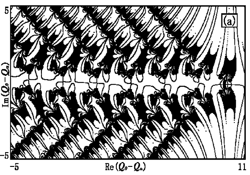
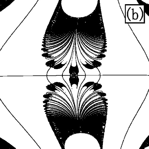
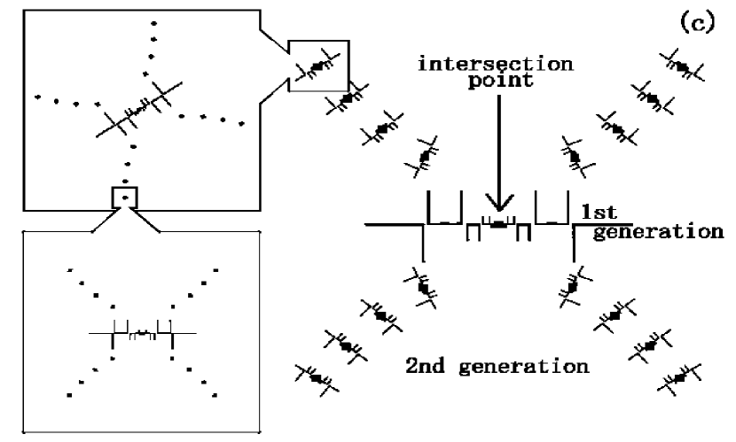
Figure 3: (a) ${\cal M}_{n}$ on the initial-value plane ${\cal I}$ for $n=10$. (b) The structure of ${\cal M}_{n}$ found in any small area on ${\cal I}$ where branches are densely aggregated. (c) Schematic representation of (b). Chain-like structures have a hierarchical configuration in ${\cal M}_{n}$. A solid square located at the center of each chain-like structure represents an element of ${\cal I}\cap{\cal W}^{s}(0,0)$.

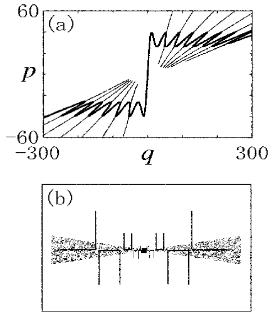
Figure 4: (a) The $n$-step iteration of ${\cal M}_{n}\cap\Delta{\cal I}$ for $n=10$, projected on real phase space. Bold and thin parts almost agree with ${\cal W}^{u}(0,0)$ in real and complex phase spaces respectively (in the thin part, those points which have quite large $\hbox{Im}\,p_{n}$ are omitted). (b) Schematic representation of ${\cal M}_{n}\cap\Delta{\cal I}$. The center dot represents a point in $M$. Hatched and non-hatched parts correspond to the bold and thin parts in (a) respectively.

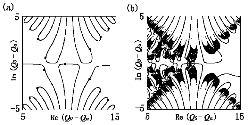
Figure 5: ${\cal M}_{n}$ for (a) $n=2$ and (b) $n=10$, in the same range of the plane ${\cal I}$. In (a), the central five branches forms a chain-like structure, which is the only chain-like structure at $n=2$. Each filled square represents a point in $M$. As $n$ increases, branches are densely aggregated in the neighbourhood of each filled square as shown in (b). When enlarging the neighbourhood, one can always find the configuration of branches shown in Fig. 3(b).

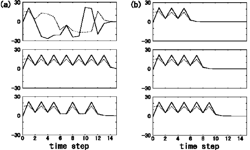
Figure 6: A variety of behaviors exhibited by orbits launching from $M$. Solid and broken lines represent $\hbox{Re}\,q$ and $\hbox{Im}\,q$ respectively. In (b), the initial points of the trajectories belong to the 6th, 8th, and 10th generations respectively in the order from the top row to the bottom one.

The hierarchical configuration of branches in ${\cal M}_{n}$ can be understood more clearly by relating it to stable and unstable manifolds in complex domain. We will show two facts: first, chain-like structures are created by the iteration of a small area element along ${\cal W}^{s}(0,0)$ and ${\cal W}^{u}(0,0)$. Second, the intersection ${\cal I}\cap{\cal W}^{s}(0,0)$ forms the main frame of the hierarchical configuration of branches. In order to see these facts, we use the notation:

$$M = {\cal I}\cap{\cal W}^{s}(0,0).$$ (14)

In the following, we mean a manifold with a real 1 dimension (resp. real 2 dimensions) by a “curve” (resp. “surface”).

When the classical map $f$ is extended to the complex phase space ${\mathbb{C}}^{2}$, both ${\cal W}^{s}(0,0)$ and ${\cal W}^{u}(0,0)$ are surfaces in the complex domain at least locally. Since the initial-value plane ${\cal I}$ is also the same dimensional surface, the dimension of the intersection $M$ is lower than 1 in general, i.e., the intersection is neither a set of curves nor a surface, but may be fractal like the Cantor set, whose Hausdorf dimension may be between 0 and 1. Let $(q_{0},p_{0})$ be an element of $M$, and $\Delta{\cal I}$ be a small neighbourhood of $(q_{0},p_{0})$ on the plane ${\cal I}$. As the time proceeds, the orbit of $(q_{0},p_{0})$ converges to the origin $(0,0)$ by definition. On the other hand, the iteration of $\Delta{\cal I}$ approaches $(0,0)$ at the initial time stage, however, it is in turn spread along ${\cal W}^{u}(0,0)$, and at a sufficiently large time step, it almost converges to ${\cal W}^{u}(0,0)$. We note that this process is not specific to our system, but the one that the stable and unstable manifolds always have. Such a process takes place also in real-domain dynamics or even in integrable one.

According to this mechanism and the conditions in (9), one may expect that for a sufficiently large time step $n$, the $n$-step iteration of ${\cal M}_{n}\cap\Delta{\cal I}$ almost agrees with a set:

$${\cal W}^{u}(0,0)\cap\{(q,p)\in{\mathbb{C}}^{2}\,\,|\,\,\hbox{Im}\,q=0\}.$$ (15)

Even in the case of $n=10$, the $n$-step iteration of ${\cal M}_{n}\cap\Delta{\cal I}$, which is projected on the real phase space in Fig. 4(a), gives a sufficiently close manifold to that presented by (15).

The bold and thin parts represent the parts of the final manifold which almost coincide with the set (15) in real and complex phase spaces respectively. This means that the bold part have sufficiently small imaginary part of final momentum compared to that of the thin part. Fig. 4(b) shows $\Delta{\cal I}$ and the schematic representation of ${\cal M}_{n}$. The center dot represents $(q_{0},p_{0})$ appearing in the above process. Hatched part and non-hatched part correspond to the bold and thin parts in Fig. 4(a), respectively. Neighbouring branches are connected with each other via caustics defined by $\partial q_{n}/\partial Q_{0}|_{P_{0}}=0$. The caustics are created by the oscillations of the real-domain ${\cal W}^{u}(0,0)$.

In this way, the creation of a chain-like structure can be understood by considering the behavior of a small area element first approaching real phase space with the guide of ${\cal W}^{s}(0,0)$, then spreading over ${\cal W}^{s}(0,0)$. In particular, the direction in which the real-domain ${\cal W}^{u}(0,0)$ stretches the area element determines the direction of the chain-like structure on the plane ${\cal I}$.

It was found that a chain-like structure on the plane ${\cal I}$ is always created around a point in $M$. Fig. 5 shows the creation of chain-like structures around the points in $M$ as the time step proceeds. In Fig. 3(c), the points in $M$ are represented by filled squares. That is to say, the hierarchical configuration of chain-like structures implies those of the points in $M$. Accordingly, $M$ constitutes the main frame of ${\cal M}_{n}$, and the notion of generation is also assigned to each point in $M$.

Since, as mentioned above, the iteration of initial points in chain-like structures to real phase space is described by orbits launching from $M$, the structure of such orbits will tell us that of orbits launching from ${\cal M}_{n}$, the latter structure is necessary for our semiclassical analysis. The study of orbits on the stable and unstable manifolds is suitable for more canonical arguments since they are compatible with the theory of dynamical systems Katok .

Fig. 6 shows a variety of itineraries of the orbits launching from $M$. In Fig. 6(a), the top row shows a typical behavior observed in $M$, where both $\hbox{Re}\,q$ and $\hbox{Im}\,q$ oscillate in an erratic manner for some initial time steps and eventually approach the origin. Regular itineraries such as periodic oscillations coexist among stochastic itineraries as shown in the middle row, where an approximately periodic 2 behavior is seen. Another type of orbit is shown in the bottom row, where the trajectory first oscillates with period 2 and then turns into a periodic 3 motion. The close relation between itinerating behaviors and the notion of generation can be seen clearly in the case of periodic oscillations, as shown in Fig. 6(b). In each row of the figure, the period for which a trajectory oscillates agrees with the generation of the initial point of the trajectory.

II.4 Emergence of Homoclinic Tanglement in Complex Phase Space

Here we will show that the hierarchical structure of $M$, which is the main frame of ${\cal M}_{n}$, is the manifestation of complex-domain chaos. First it is shown that homoclinic tanglement emerges in the complex domain. The laminations of ${\cal W}^{s}(0,0)$ and ${\cal W}^{u}(0,0)$ are densely developed around the origin $(0,0)$ in the complex domain, and they are described by the notion of generation. Then it is explained that the hierarchical structure of $M$ is created as a consequence of the emergence of the complex homoclinic tanglement.

In order to study the structure of complex phase space, we introduce coordinates on ${\cal W}^{s}(0,0)$ and ${\cal W}^{u}(0,0)$ as follows. Let $\Phi_{s}$ and $\Phi_{u}$ be conjugation maps from a complex plane ${\mathbb{C}}$ to ${\cal W}^{s}(0,0)$ and ${\cal W}^{u}(0,0)$ respectively, which satisfy the relations:

$$f_{s}(\xi_{s}) = {\lambda}^{-1}\xi_{s}\quad\text{ for }\xi_{s}\in{\mathbb{C}},$$ (16a)

$$f_{u}(\xi_{u}) = \lambda\xi_{u}\qquad\text{ for }\xi_{u}\in{\mathbb{C}},$$ (16b)

where $f_{s}$ and $f_{u}$ are

$$f_{s}(\xi) = \left(\Phi_{s}^{-1}\,f\,\Phi_{s}\right)(\xi),$$ (17a)

$$f_{u}(\xi) = \left(\Phi_{u}^{-1}\,f\,\Phi_{u}\right)(\xi),$$ (17b)

and $\lambda$ denotes the maximal eigenvalue of the tangent map on the unstable fixed point $(0,0)$ Gelfreich1 . The above coordinates $\xi_{s}$ and $\xi_{u}$ are normalized in the sense that the classical map $f$ is represented by a linear transformation on each coordinate. The set of homoclinic points associated with the origin, ${\cal W}^{s}(0,0)\cap{\cal W}^{u}(0,0)$, is obtained numerically on these coordinates as shown in Fig. 7.

In each of Fig. 7(a) and (b), enlarging the neighbourhood of the origin by ${\lambda}^{n}$ times $(n\geq 1)$, one obtains the same figure with the original one due to the relations in (16). This means that the homoclinic points are accumulated around the origin $(0,0)$, in other words, the laminations of ${\cal W}^{u}(0,0)$ and ${\cal W}^{s}(0,0)$ in the complex domain are densely developed around the origin. It is a direct numerical evidence of the emergence of homoclinic tanglement in complex phase space, and thus null topological entropy in real phase space does not always exclude the existence of chaos in complex domain.

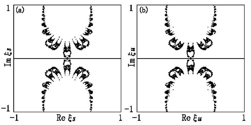
Figure 7: The set of homoclinic points associated with the unstable fixed point $(0,0)$ plotted on (a) ${\cal W}^{s}(0,0)$ and (b) ${\cal W}^{u}(0,0)$. The origin of each figure corresponds to the unstable fixed point, and the horizontal axis through the origin is included in real phase space.

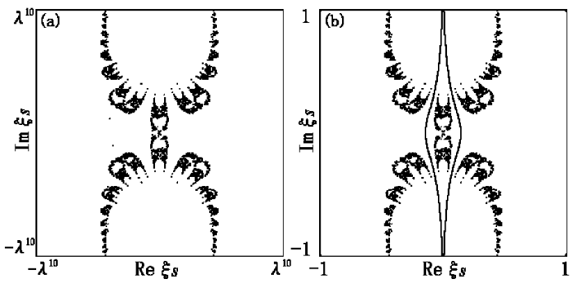
Figure 8: (a) The intersection $M$ plotted on the $\xi_{s}$ plane. (b) The domain $D$ plotted on the $\xi_{s}$ plane with the set of homoclinic points superposed.

Fig. 8(a) shows $M$ plotted on the $\xi_{s}$ coordinate. Similarity to Fig. 7(a) is evident, which suggests that the creation of the hierarchical configuration of $M$ on the plane ${\cal I}$ is due to the emergence of homoclinic tanglement in the complex domain. The relation between the structures of $M$ and the complex homoclinic tanglement is made more clear by the notion of generation, which we have already introduced. To see the relation, the precise definition of generation is given as follows. Let $D$ be a connected domain in the $\xi_{s}$ plane satisfying the conditions:

$$(0,0) \in D,$$ (18a)

$$f_{s}(D) \subset D,$$ (18b)

where $f_{s}$ is the linear transformation defined in (16a). Then denoting $D\backslash f_{s}(D)$ by $\tilde{D}$, the $\xi_{s}$ plane is decomposed into a family of disjoint domains as follows:

$$\bigsqcup_{n\in{\mathbb{Z}}}f_{s}^{n}(\tilde{D}) = {\mathbb{C}}-\left\{(0,0)\right\},$$ (19a)

$$f_{s}^{m}(\tilde{D})\cap f_{s}^{n}(\tilde{D}) = \phi\quad(m\neq n).$$ (19b)

Thus for any point $\xi_{s}$ in this plane except $(0,0)$, there exist a unique integer $n$ such that $\xi_{s}\in f_{s}^{-n}(\tilde{D})$. We define the generation of the point $\xi_{s}$ as such an integer $n$.

The shape of the domain $D$ is shown in Fig. 8(b). Note that the relations in (19) hold irrespective of the shape of $D$. In our earlier publication OnishiShudoIkedaTakahashi1 , $D$ was chosen as a disk. In the present study, another choice of $D$ is proposed. More precise definition of $D$ is given in Sec. II.5 in the context of the construction of symbolic dynamics.

For any point in the neighbourhood of the origin in $D$, the forward orbit approaches the origin straightforwardly at an exponential rate in the original coordinate $(q,p)$. For any point in the $n$-th generation $(n\geq 1)$, it takes at least $n$ steps until the orbit starts to approach the origin exponentially, and thus it can exhibit a variety of behaviors during its itinerary. That is why the oscillations shown in Fig. 6 are related with the generations.

Fig. 9 shows the generations in real phase space. On one hand, in real-domain dynamics, a single iteration of the map $f$ creates a single oscillation of ${\cal W}^{s}(0,0)$. On the other hand, by definition, any point of ${\cal W}^{s}(0,0)$ in any generation is mapped by $f$ to another point in the neighbouring generation. Therefore in real phase space, each generation corresponds to a single oscillation of ${\cal W}^{s}(0,0)$.

In the complex domain, however, as seen in Fig. 3(c), higher generations describe finer scales of the hierarchical configuration of $M$ on the plane ${\cal I}$. Fig. 3(c) also shows that for any point of $M$ and in its small neighbourhood on the plane ${\cal I}$, the number of the members in $M$ which are included in individual generations increases exponentially with the generations. This situation clearly shows that the homoclinic tanglement of ${\cal W}^{s}(0,0)$ and ${\cal W}^{u}(0,0)$ creates the hierarchical configuration of $M$ on the plane ${\cal I}$.

It should be noted that real-domain chaos, if it exits, also creates the hierarchical configuration. Fig. 10 shows a simple analogy of our present situation with a horse shoe map on a two-dimensional plane. One-dimensional ${\cal W}^{s}(0,0)$ and ${\cal W}^{u}(0,0)$ create homoclinic tanglement, and the one-dimensional bar across the tanglement corresponds to our initial-value plane ${\cal I}$. In this case, both ${\cal I}\cap{\cal W}^{s}(0,0)$ and ${\cal I}\cap{\cal W}^{u}(0,0)$ form the Cantor sets, and the fractal structures of these intersections are originated from densely developed laminations of ${\cal W}^{s}(0,0)$ and ${\cal W}^{u}(0,0)$. The interval on ${\cal W}^{s}(0,0)$ indicated by a bold curve corresponds to our domain $D$. Replacing ${\mathbb{C}}$ in (19a) by ${\mathbb{R}}$, one can define generations in a similar way. Due to the horse shoe dynamics on this plane, ${\cal W}^{s}(0,0)$ in the $n$-th generation has $2^{n}$ intersection points with the initial-value bar.

In this sense, whether in real domain or in complex one, the hierarchical configuration of ${\cal I}\cap{\cal W}^{s}(0,0)$ on the plane ${\cal I}$ is nothing but the manifestation of chaos. In particular, the emergence of the above configuration in the complex domain is a piece of evidence for complex-domain chaos. Once we know that chaos exists also in the complex domain, the methodology studying chaos in the real domain can be applied to the analysis on the complex domain. In particular, symbolic dynamical description of orbits, which is available if one finds a proper partition of phase space to define it, is a standard technique in the theory of dynamical systems Katok , and can be very useful tool to analyze complicated phase space structures. Homoclinic orbits are also describable in terms of the symbolic dynamics, so our strategy to study the hierarchical configuration of $M$ hereafter is to take the symbolic description of homoclinic orbits.

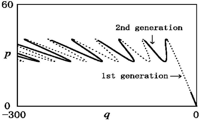
Figure 9: Generations of ${\cal W}^{s}(0,0)$ in real phase space. The bold and dotted curves represent even and odd generations respectively, except for the bold part emanating from the origin, which represents the generations lower than or equal to zero. The generation increases monotonically as $q\rightarrow-\infty$.

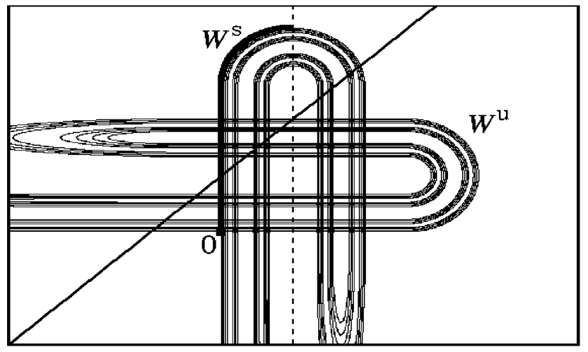
Figure 10: The horse-shoe map defined on a two-dimensional plane. The one-dimensional bar across the tanglement corresponds to our initial-value plane ${\cal I}$, and the bold curve on ${\cal W}^{s}(0,0)$ corresponds to our domain $D$. The dotted line is the boundary of partition which creates binary codes.

II.5 Symbolic Description of Complex Orbits

We will explain the symbolic description of the complex homoclinic orbits and its application to the symbolic description of semiclassical candidate orbits. The symbolic description of homoclinic orbits contains the construction of symbolic dynamics which works effectively and the estimation of imaginary parts of actions for the homoclinic orbits. We here present only the final results of our study on this description, and the detailed explanation is given in Sec. III. On the basis of the results, the symbolic description of semiclassical candidate orbits is discussed as follows. First the orbits launching at $M\,(={\cal I}\cap{\cal W}^{s}(0,0))$ are encoded into symbolic sequences. We compare both configurations of homoclinic points and the elements of $M$, on the $\xi_{s}$ coordinate set on ${\cal W}^{s}(0,0)$. A clear similarity between both configurations enables us to find, for each element of $M$, a homoclinic point located in the neighbourhood of the element of $M$. Since the homoclinic point is encoded into a symbolic sequence, we encode the element of $M$ into this symbolic sequence. Then semiclassical candidate orbits are encoded into symbolic sequences. Since the behaviors of orbits launching at a single chain-like structure are described by the behavior of the orbit of an element of $M$ located at the center of the chain-like structure, we assign the symbolic sequence of the element of $M$ to the initial points of the chain-like structure.

Symbolic dynamics is usually constructed by finding a generating partition ${\cal G}$, which is the partition of phase space satisfying the relation:

$$\bigvee_{n=-\infty}^{+\infty}f^{n}({\cal G}) = \epsilon_{0},$$ (20)

where the l.h.s. is the product of all partitions created by the iterations of ${\cal G}$, and the r.h.s. is the partition of phase space into its individual points Katok (here we should consider the “phase space” as the closure of a set of homoclinic points). Roughly speaking, ${\cal G}$ is the partition of phase space such that each separated component of phase space corresponds to a symbol and for every bi-infinite sequence of symbols there may at most exist one trajectory of the original map.

In our case, a partition of complex phase space is defined in terms of a phase part of the gradient of the potential function:

$$V^{\prime}(q) = -2\gamma k\exp\left[-A(q)-{\rm i}B(q)\right],$$ (21)

where $A(q),B(q)\in{\mathbb{R}}$. The boundaries of our partition are defined as follows:

$$\left\{(q,p)\in{\mathbb{C}}^{2}\,\,|\,\,B(q)=\left[2\nu xy-(3x+1)y/2\right]\pi\right\},$$ (22)

where $\nu$ is arbitrary positive integer, and $(x,y)$ is an element of the set:

$${\cal T} = \left\{(+1,+1),(-1,+1),(-1,-1),(+1,-1)\right\}.$$ (23)

The intersection between the $q$ plane and the boundaries of the partition are shown in Fig. 11. Each boundary is a three-dimensional manifold according to (22), so that the intersection is a set of one-dimensional curves. $x$ and $y$ in (22) represent the signs of $\hbox{Re}\,q$ and $\hbox{Im}\,q$ of the points on a boundary respectively, i.e., the pair of $x$ and $y$ specifies the quadrant of the $q$ plane where the $q$ component of the boundary is included. $\nu$ is the “distance” between the boundary and the origin $(0,0)$, in the sense that the axis $\hbox{Re}\,q=\hbox{Im}\,q$ on the $q$ plane intersects the boundary at $q\approx(x\sqrt{\nu\pi/\gamma},y\sqrt{\nu\pi/\gamma})$ for $\nu\gg 1$.

Then our partition, denoted by ${\cal P}$, is defined as a set of phase space components as follows:

$${\cal P} = \left\{U(x,y,\nu)\,\,|\,\,(x,y,\nu)\in{\cal S}\right\},$$ (24a)

$${\cal S} = ({\cal T}\otimes{\mathbb{N}})\cup\{(0,0,0)\},$$ (24b)

where $U(x,y,\nu)$ for $(x,y,\nu)\in{\cal T}\otimes{\mathbb{N}}$, whose $q$ component is displayed in Fig. 11, denotes the region enclosed by two boundaries associated with $(x,y,\nu)$ and $(x,y,\nu+1)$, and $U(0,0,0)$ denotes the complement of the union of all components associated with $(x,y,\nu)\in{\cal T}\otimes{\mathbb{N}}$. The origin of phase space, $(0,0)$, is included in $U(0,0,0)$.

Fig. 12 shows the $\xi_{s}$ plane divided by $f^{n}({\cal P})$ for $n=0$ and 1. The central domain in Fig. 12(a) is the domain $D$, as is explained in Sec. II.4. The domain $D$ is defined as a connected domain in $U(0,0,0)\cap{\cal W}^{s}(0,0)$ which includes the origin $(0,0)$. If $f^{n}({\cal P})$ for any $n\geq 0$ divides clearly the set of homoclinic points displayed here, then ${\cal P}$ is the generating partition, i.e., the relation (20) holds for ${\cal P}$ (it is sufficient to consider the case of $n\geq 0$ since any homoclinic point is mapped to the region displayed in Fig. 12(a) by the iterations of the map).

On one hand, $f^{n}({\cal P})$ for $n=0$ divides a set of homoclinic points clearly as shown in Fig. 12(a). This means that our partition is a reasonable approximation of the generating partition ${\cal G}$. So by means of ${\cal P}$, we can construct a symbolic dynamics which works effectively. On the other hand, there are some regions in the $\xi_{s}$ plane where $f^{n}({\cal P})$ for $n\geq 1$ fails to divide the set of homoclinic points clearly. In such regions, it may be necessary to improve our partition to obtain the generating partition, and it is our future problem. Note that our complex dynamics is not proven to be sufficiently chaotic, i.e., hyperbolic, and that the existence of the generating partition for non-hyperbolic systems is an open problem. The improvement of the partition is of a mathematical interest, however, as actually demonstrated below, the present definition of ${\cal P}$ is sufficient for our semiclassical analysis.

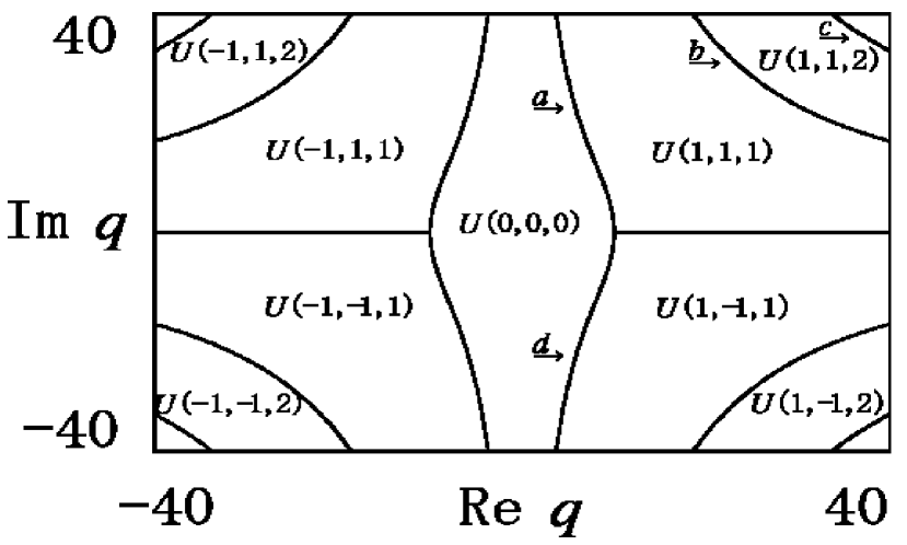
Figure 11: Intersection between the $q$ plane and the boundaries of the partition. The curves labeled by $a,b,c,$ and $d$ indicate the boundaries associated with $(x,y,\nu)=(1,1,1),(1,1,2),(1,1,3),$ and $(1,-1,1)$ respectively.

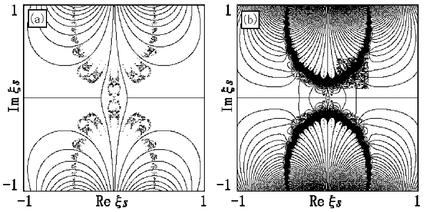
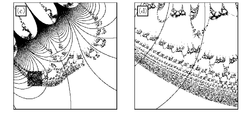
Figure 12: Boundaries of (a) the partition ${\cal P}$ and (b) its forward iteration $f({\cal P})$ plotted on ${\cal W}^{s}(0,0)$, with homoclinic points superposed. The generations of the homoclinic points displayed are lower than or equal to 1. (c) The enlarged figure of the hatched part of (b). The boundaries of $f({\cal P})$ fails to divide the set of homoclinic points clearly, in the hatched part of (c). (d) The enlarged figure of the hatched part of (c). Homoclinic points are aggregated densely like a thick band. The boundary curves might touch the set of homoclinic points.

In terms of the partition ${\cal P}$, each homoclinic point is encoded into a bi-infinite symbolic sequence of the form:

$$\!\!\!\!\!\!\!\!\!\!\!\ldots O\,\,O\,a_{-n}\,a_{-(n-1)}\ldots a_{-1}\,\,.\,\,a_{0}\,\,\,a_{1}\ldots a_{n}\,\,O\,\,O\,\ldots,$$ (25)

where $O=(0,0,0)$, $n\in{\mathbb{N}}$, and $a_{k}\in{\cal S}\,\,(|k|\leq n)$. The symbol $a_{k}$ stands for a phase space component denoted by $U(a_{k})$ which contains the $k$-th iteration of the homoclinic point, whose initial location is in $U(a_{0})$. The finite sequence of $a_{k}\,\,(|k|\leq n)$ is accompanied with semi-infinite sequences of $O$’s in both sides. It reflects that any homoclinic point approaches the origin of phase space by forward and backward iterations of the map $f$. In particular, homoclinic points included in $D$ are encoded into symbolic sequences of the form:

$$\ldots O\,\,O\,\,a_{-n}\,a_{-(n-1)}\ldots a_{-1}\,\,.\,\,O\,\,O\ldots,$$ (26)

where $n\in{\mathbb{N}}$ and $a_{k}\in{\cal S}\,\,(0<k\leq n)$. Any symbol in the r.h.s. of the decimal point is $O$, since the forward trajectory is always included in a component $U(O)$ due to the definition of $D$.

Further investigation of symbolic dynamics, which is presented in Sec. III, enables us to estimate the amount of imaginary parts of actions gained by homoclinic orbits. Let $w$ a homoclinic point which has a symbolic sequence of the form (25). When we denote $a_{k}=(x_{k},y_{k},\nu_{k})$ for $k\in{\mathbb{Z}}$, the imaginary part of action gained by the forward trajectory of $w$, denoted by $s(w)$, is estimated as follows:

$$s(w) = \sum_{k=1}^{+\infty}\hbox{Im}\left[T(p_{k-1})-V(q_{k})\right]$$

$$\approx \frac{\pi}{\gamma}\sum_{k=1}^{+\infty}(x_{k}\nu_{k}^{1/2}-x_{k-1}\nu_{k-1}^{1/2})(y_{k}\nu_{k}^{1/2}-y_{k-1}\nu_{k-1}^{1/2}),$$

where $\gamma$ is a parameter of the potential function $V(q)$.

From these results, we discuss the symbolic description of semiclassical candidate orbits. To this end, we display schematically the configurations of homoclinic points and the elements of $M$, which are shown in the previous Figs. 7(a) and 8(a). The configurations can be seen clearly by introducing graphs on the $\xi_{s}$ coordinate of ${\cal W}^{s}(0,0)$, whose vertices represent the homoclinic points or the elements of $M$.

The configuration of the homoclinic points in the domain $D$ is represented by a graph $K_{\infty}$ defined as follows. First, by a graph $K_{1}$ which is shown in Fig. 13(a), we represent homoclinic points which have symbolic sequences of the form:

$$\ldots O\,\,O\,\,a_{-1}\,\,.\,\,O\,\,O\ldots\quad(a_{-1}\in{\cal S}).$$ (28)

Second, we attach smaller copies of $K_{1}$ to each vertex of the original $K_{1}$ to obtain a graph $K_{2}$ which is shown in Fig. 13(b). By the graph $K_{2}$, we represent homoclinic points which have symbolic sequences of the form:

$$\ldots O\,\,O\,\,a_{-2}\,\,a_{-1}\,\,.\,\,O\,\,O\ldots\quad(a_{-2},a_{-1}\in{\cal S}).$$ (29)

In a similar way, a graph $K_{n}$ is obtained for any integer $n\geq 3$ by attaching much smaller copies of $K_{1}$ to each vertex of $K_{n-1}$. Since inclusions hold as $K_{1}\subset K_{2}\subset K_{3}\subset\ldots$, we finally obtain a graph $K_{\infty}$ which is shown in Fig. 14, as the union of the graphs $K_{1},\,K_{2},\,K_{3},\ldots$. $K_{\infty}$ is a tree graph, i.e., there is no loop on the graph.

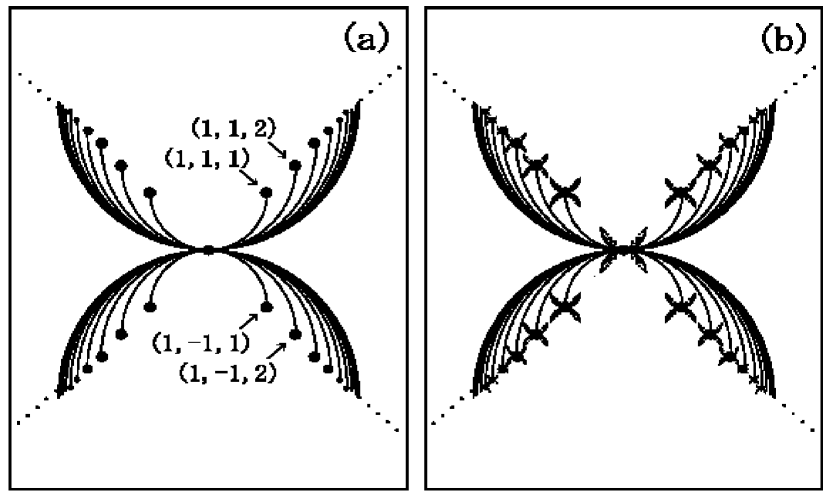
Figure 13: Graphs (a) $K_{1}$ and (b) $K_{2}$ representing homoclinic points which have symbolic sequences of forms $\ldots O\,O\,a_{-1}\,\,.\,\,O\,O\ldots$ and $\ldots O\,O\,a_{-2}\,\,a_{-1}\,\,.\,\,O\,O\ldots$ respectively, where $a_{-2},\,a_{-1}\in{\cal S}$. In (a), the center vertex corresponds to the case of $a_{-1}=O$, and the vertices in the upper-right side and in the lower-right one correspond respectively to the cases of $a_{-1}=(1,1,\nu)$ and $a_{-1}=(1,-1,\nu)$ with $\nu\in{\mathbb{N}}$, and so on.

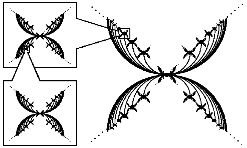
Figure 14: The graph $K_{\infty}$ representing homoclinic points included in the domain $D$. Hierarchical configurations of vertices can be seen by enlarging the neighbourhood of any vertex.

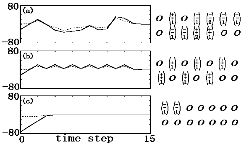
Figure 15: The orbits launching from $M$, and symbolic sequences assigned to the initial points of the orbits. The upper and lower signs in each symbol denotes $x$ and $y$ in (24) respectively, and the integer denotes the value of $\nu$. A semi infinite part, $O\,\,O\,\,O\ldots$, is omitted in each sequence. Solid and broken lines represent $\hbox{Re}\,q$ and $\hbox{Im}\,q$ respectively. The trajectories show (a) erratic motions, (b) approximately 2-periodic motions, and (c) monotonical approach to real phase space.

Next we consider the configuration of the elements of $M$. As shown in Figs. 7(a) and 8(a), there are clear similarities between configurations of homoclinic points and the elements of $M$. We define $M_{n}$ as a subset of $M$ such that the members belong to generations lower than $n$. Then we observed numerically the following two facts: one is that on ${\cal W}^{s}(0,0)$, the elements of $M_{n}$ for $n\geq 3$ have the same configuration as a graph $K_{n-2}$ ($M_{n}$ for $n=2$ has only a single element, and $M_{n}$ for $n=1$ is null). The other is that on the plane ${\cal I}$, the elements of $M_{n}$ are located at the centers of chain-like structures in ${\cal M}_{n}$ (see Fig. 3(c)).

In the case of homoclinic points, each vertex of $K_{n-2}$ corresponds to a symbolic sequence of the form:

$$\ldots O\,\,O\,\,a_{-(n-2)}\,\,a_{-(n-3)}\ldots\,a_{-1}\,\,.\,\,O\,\,O\,\ldots.$$ (30)

Then to each point of $M_{n}$, one can assign formally a semi infinite symbolic sequence of the form:

$$a_{-(n-2)}\,\,a_{-(n-1)}\,\,\ldots\,\,a_{-1}\,\,O\,\,O\ldots.$$ (31)

Fig. 15 shows some trajectories launching from $M$ and symbolic sequences of the form (31) assigned to the initial points of the trajectories. The signs and amplitudes of the $q$ components at each time step are well described by $(x,y)$’s and $\nu$’s of the corresponding symbols. This means that there are clear similarities between motions of both trajectories launching from $M$ and a set of homoclinic points. More precisely, for an element of $M$ which has a symbolic sequence of the form (31), the forward trajectory is well approximated by that of a homoclinic point which has a symbolic sequence of the form:

$$\ldots O\,\,O\,\,.\,\,a_{-(n-2)}\,\,a_{-(n-1)}\ldots\,a_{-1}\,\,O\,\,O\,\ldots.$$ (32)

In this way, the elements of $M_{n}$ are described by symbolic sequences. To the chain-like structure in ${\cal M}_{n}(\subset{\cal I})$ which is associated with each element of $M_{n}(\subset{\cal W}^{s}(0,0))$, we assign the same symbolic sequence as the element of $M_{n}$, since as stated in Sec. II.3, the motions of trajectories launching from a single chain-like structure are well approximated, till they start to spread along the real domain ${\cal W}^{u}(0,0)$, by the motion of a trajectory launching from an element of $M$ located at the center of the chain-like structure. Then chain-like structures in ${\cal M}_{n}$ are also described by symbolic sequences of the form (31).

Finally, we discuss the estimation of imaginary parts of actions gained by semiclassical candidate orbits. By making use of the above mentioned similarities between $M$ and a set of homoclinic points, for an element of $M_{n}(\subset M)$ which has a symbolic sequence:

$$a_{0}\,\,a_{1}\,\,a_{2}\ldots a_{n-3}\,\,O\,\,O\ldots,$$ (33)

(note that the notation is slightly different from (31)) we evaluate the imaginary part of action of its orbit by a homoclinic orbit with a symbolic sequence:

$$\ldots O\,\,O\,\,.\,\,a_{0}\,\,a_{1}\,\,a_{2}\ldots a_{n-3}\,\,O\,\,O\ldots.$$ (34)

Due to this evaluation, the former imaginary part of action is estimated by applying (LABEL:estimation_formula_of_ImS) to the symbolic sequence (33).

For each trajectory launching from a single chain-like structure in ${\cal M}_{n}$, we approximate the imaginary part of action as that of the trajectory launching from the element of $M_{n}$ located at the center of the chain-like structure. In this way, we can estimate the imaginary parts of actions gained by semiclassical candidate orbits. Though there are branches in ${\cal M}_{n}$ which are not included in any chain-like structure, semiclassical contributions from them are negligible. See the discussion in Sec. II.6.

II.6 Reproduction of Tunneling Wave Functions

Semiclassical wave functions are constructed from significant tunneling orbits selected according to the amounts of imaginary parts of actions. The semiclassical mechanism of the tunneling process is explained by the structure of complex phase space.

The wave function $\langle q_{n}|U^{n}|q_{\alpha},p_{\alpha}\rangle$ given in (7) is constructed by two steps: First, out of $M_{n}(\subset M)$ the elements are picked up such that the imaginary parts of actions estimated by (LABEL:estimation_formula_of_ImS) are minimal. Second, the Van Vleck’s formula in (LABEL:Van_Vleck_formula_a) is evaluated for the initial points in chain-like structures associated with these elements of $M_{n}$. Before picking up the elements out of $M_{n}$, the Stokes phenomenon Heading should be taken account of. Following the prescription given in Ref. ShudoIkeda3 , we found that chain-like structures which have unphysical contributions to the wave function are associated with elements of $M_{n}$ whose symbolic sequences include symbols of the form $(1,-1,\nu)$ or $(-1,1,\nu)$ with $\nu\in{\mathbb{Z}}$. At least, the chain-like structures which attain exponentially large semiclassical amplitudes are in this case. The justification is our future problem. See, the Discussion.

After excluding such elements from $M_{n}$, we have an ordering for elements of $M_{n}$:

$$w_{0}\,\,\,\,w_{1}\,\,\,\,w_{2}\,\,\ldots,$$ (35)

such that inequalities hold:

$$0\leq s(w_{0})\leq s(w_{1})\leq s(w_{2})\leq\ldots,$$ (36)

where $s(w_{k})$ for $k=0,1,2,\ldots$ represents the imaginary part of action estimated by (LABEL:estimation_formula_of_ImS) for the forward trajectory of $w_{k}$.

From the Appendix II, it is seen that $w_{0}$, which is primarily significant in $M_{n}$ for the wave function, has a symbolic sequence:

$$O\,\,O\,\,O\ldots,$$ (37)

and the members of $\{w_{1},w_{2},\ldots,w_{2(n-2)}\}$, which are secondarily significant in $M_{n}$, have symbolic sequences of the form:

$$b\,\,\,b\,\,\,b\,\ldots\,b\,\,\,b\,\,\,O\,\,O\,\,O\ldots,$$ (38)

where $b=$ $(1,1,1)$ or $(-1,-1,1)$. Due to (31), the length of $\,b\,\,b\,\,b\,\ldots\,b\,\,b\,$ varies from 1 to $n-2$, and the member of $\{w_{1},w_{2},\ldots,w_{2(n-2)}\}$ which has $\,b\,\,b\,\,b\,\ldots\,b\,\,b\,$ of length $k-2\,\,(k\leq n)$ belongs to the $k$-th generation. From (LABEL:estimation_formula_of_ImS) it is estimated that $s(w_{1})=s(w_{2})=\ldots=s(w_{2(n-2)})$.

We observed that the orbits $\{w_{0},\,\,w_{1},\ldots,w_{2(n-2)\}}$ behave as follows. The orbit $w_{0}$ converges to the origin of phase space exponentially, so that it gains only small imaginary part of action. The orbits $\{w_{1},\,\,w_{2},\ldots,w_{2(n-2)}\}$ first explore the vicinity of real phase space till the sequence $\,b\,\,b\,\,b\ldots b\,\,b$ terminates, and then converge to the origin exponentially. Such motions yield much smaller imaginary parts of actions than flipping motions in complex domain. The latters are generic trajectories launching from $M$. The motions of homoclinic orbits whose symbolic sequences include sub sequences of the form (38) are investigated in Sec. III. There it is found that such homoclinic orbits explore the vicinity of real phase space. The motions of the orbits of $w_{1},\,\,w_{2},\ldots,w_{2(n-2)}$ reflect those of homoclinic orbits.

Fig. 16 shows quantum and semiclassical wave functions for $n=10$, the latter of which is constructed by taking account of the contributions from chain-like structures associated with $w_{0},\,\,w_{1},\ldots,w_{2(n-2)}$. Both functions are in excellent agreement. The contributions from the other chain-like structures are much smaller than those from the chain-like structures associated with $w_{0},\,\,w_{1},\ldots,w_{2(n-2)}$. In fact, the squared amplitudes of them are of order $\sim 10^{-50}$ at most. In particular, the contributions from trajectories which exhibit flipping or oscillatory motions are negligible, as shown in Fig. 17.

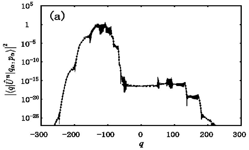
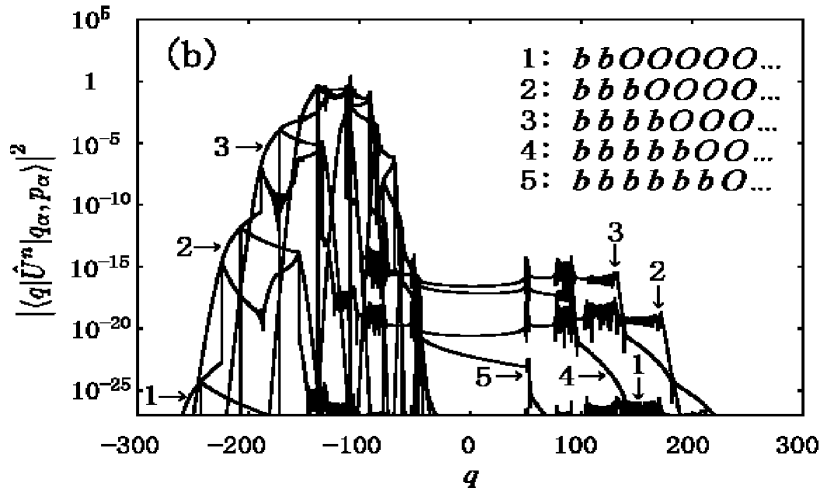
Figure 16: (a) The squared amplitudes of the quantum and semiclassical wave functions for $n=10$, represented by dotted and solid curves respectively. Note that both curves are superposed. (b) Individual contributions from chain-like structures to the semiclassical wave function shown in (a). For some components, symbolic sequences assigned to chain-like structures are presented, where $b=(-1,-1,1)$.

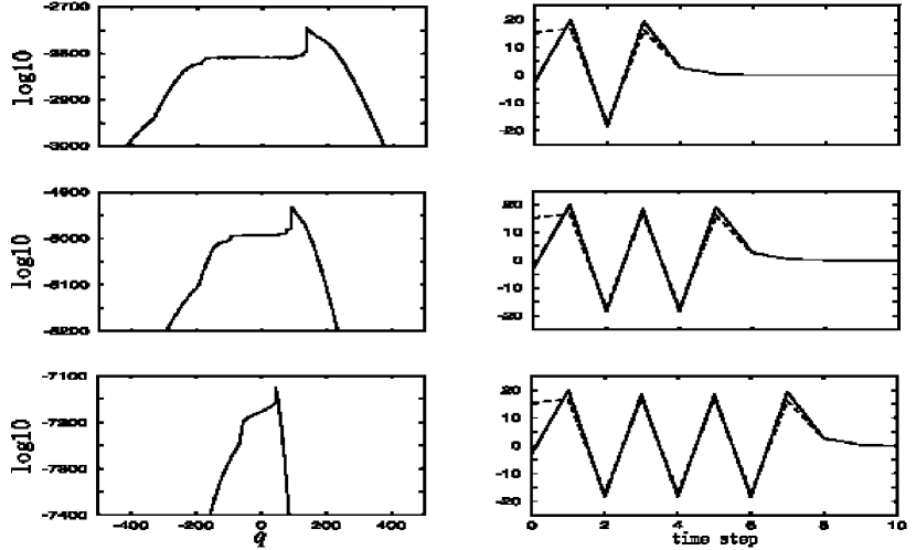
Figure 17: Squared amplitudes of the semiclassical components (the l.h.s.) which come from chain-like structures associated with the elements of $M$ whose trajectories exhibit oscillatory motions (the r.h.s.). Solid and broken lines in the r.h.s. represent $\hbox{Re}\,q$ and $\hbox{Im}\,q$ respectively. Flipping or oscillatory motions in complex phase space gain large amounts of imaginary parts of actions due to large complex momenta.

On one hand, significant chain-like structures increase linearly with the time step $n$ as seen above, and the branches included in individual chain-like structures also increase linearly with $n$, reflecting the oscillations of real domain ${\cal W}^{u}(0,0)$. So the numbers of branches which we should take into account increases algebraically with $n$. On the other hand, the number of chain-like structures in ${\cal M}_{n}$, and that of branches in ${\cal M}_{n}$ increase exponentially with $n$. Therefore only a small number of branches are significant to describe the tunneling process. The algebraic increase of the significant orbits is a consequence of the absence of real-domain chaos. When the real domain is chaotic, a small piece of manifold which has approached the real domain are stretched and folded without gaining additional imaginary part of action, so that the number of significant orbits can increase exponentially with time.

The contributions from branches not included in any chain-like structures are also negligible, such as the branches in Fig. 5(a) except the central five ones. For orbits launching from such branches in ${\cal M}_{n}$, there is no orbit launching from $M$ which guides them to real phase space within $n$ time steps. This means that these orbits have large imaginary parts of momenta at the time step $n$, so that they gain sufficiently large amounts of imaginary parts of actions. If the imaginary parts of actions are positively large, the contributions from the orbits are small enough to be negligible, or if they are negatively large, the contributions from the orbits are unphysical due to the Stokes phenomenon, so that the orbits should be excluded from the whole candidates.

The excellent agreement between both quantum and semiclassical calculations enables us to interpret semiclassically the features of tunneling wave functions. Fig. 16(b) shows a decomposition of the semiclassical wavefunction in Fig. 16(a) into components which come from individual chain-like structures. It can clearly be seen that the contributions from many chain-like structures reproduce the crossover of amplitudes in the reflected region and the staircase seen in the transmitted region. We found that erratic oscillations on each component are due to the interferences between branches included in a single chain-like structure. The symbolic sequences of the form (38) can have various lengths of $b\,\,b\,\,b\ldots b\,\,b$. The lengths of this part correspond to the generations of $w_{1},\,\,w_{2},\ldots,w_{2(n-2)}$. Thus both the staircase and the crossover of amplitudes are created by the interferences between chain-like structures belonging to different generations. In this way, the complicated tunneling amplitude is explained semiclassically by the creations of chain-like structures on the initial-value plane, and by the exponential increase of the number of chain-like structures with time (though linear increase for significant ones), which is due to the emergence of complex homoclinic tanglement.

The semiclassical mechanism of the tunneling process in our system is summarized as follows. Stable and unstable manifolds of a real-domain unstable orbit create tanglement in complex domain. The initial manifold representing a quantum initial state is located in the tanglement, so that the intersection points between the initial manifold and the stable manifold form a hierarchical structure on the initial manifold. The orbits launching from the neighbourhood of each intersection point are guided to real phase space by the stable manifold, and then spread over the unstable manifold. The number of the orbits guided to real phase space increases exponentially with time (though significant ones increase algebraically), reflecting the hierarchical structure formed by the intersection points on the initial manifold. Then the interferences between these orbits create complicated patterns in the tunneling amplitude.

III Symbolic Description of Complex Homoclinic Structure

III.1 Construction of Partition of Phase Space

Here we construct a partition of phase space which encodes homoclinic points of the origin $(0,0)$ into symbolic sequences and defines a symbolic dynamics which works effectively. The behaviors of homoclinic orbits and the estimation of imaginary parts of actions for the orbits are presented in the following Secs. III.2 and III.3 respectively.

There has been extensive studies on the construction of generating partition in real phase space Cvitanovic even in non-hyperbolic regimes ChristiansenPoliti . In such real-domain studies, the boundaries of generating partition are roughly approximated by a set of folding points created by the single-step iterations of flat manifolds. However, the extension of such working principle to complex phase space is not obvious.

In order to know the locations of the boundaries of the generating partition, we consider the iterations of flat manifolds given by the form $\{(q,p)\in{\mathbb{C}}^{2}\,|\,p=p_{0}\}$ for a complex value $p_{0}$. Fig. 18 shows the iterations of some small pieces of such a flat manifold, which exhibit a variety of behaviors depending on the initial locations of the small pieces. Since the magnitude and phase of the gradient $V^{\prime}(q)$ are controlled respectively by the functions $A(q)$ and $B(q)$ which appear in (21), the differences of the behaviors shown in the figure mainly come from the differences of the values of $A(q)$. The contour curves of $A(q)$ and $B(q)$ are shown in Fig. 19.

In order to know the locations of the boundaries of the partition far from the origin $(0,0)$, we introduce a coordinate $(u,v)$ in the $q$ plane:

$$u = \left[(\hbox{Re}\,q)^{2}-(\hbox{Im}\,q)^{2}\right]/2,$$ (39a)

$$v = \hbox{Re}\,q\cdot\hbox{Im}\,q.$$ (39b)

On this coordinate, we obtain the estimations:

$$A(q) = \gamma\left[(\hbox{Re}\,q)^{2}-(\hbox{Im}\,q)^{2}\right]-\log|q|$$ (40a)

$$= 2\gamma u+O\left(\log|u|\right)\quad\!\!\!\!\!\left(v:\hbox{fixed},\,\,|u|\,\rightarrow\,\infty\right)\!,\ \ \ \$$

$$B(q) = 2\gamma\hbox{Re}\,q\cdot\hbox{Im}\,q-\hbox{Arg}\,\,q$$ (40b)

$$= 2\gamma v+O\left(\log|v|\right)\quad\!\!\!\!\!\left(u:\hbox{fixed},\,\,|v|\,\rightarrow\,\infty\right)\!,\ \ \ \$$

or $$2\gamma v+O\left(|u|^{-1}\right)\quad\!\!\!\left(v:\hbox{fixed},\,\,|u|\,\rightarrow\,\infty\right)\!,\ \ \ \$$ (40c)

where $\gamma$ is a parameter of $V(q)$. The above estimations imply that far from the origin $(0,0)$ the magnitude and phase of $V^{\prime}(q)$ are controlled by $u$ and $v$ respectively.

On one hand, in a region of phase space with $u\gg 1$, which includes the real asymptotic region, $V^{\prime}(q)$ almost vanishes so that the behavior of a small piece of manifold there, typically observed as that of $m_{1}$ in Fig. 18, is of a free motion. On the other hand, in a region of phase space with $u\ll-1$, any small rectangle on the $(u,v)$ coordinate, $\{q\in{\mathbb{C}}\,\,|\,\,u\in[u_{0},u_{0}+\Delta u],\,v\in[v_{0},v_{0}+\Delta v]\}$, with $u_{0}\ll-1$ is mapped by $V^{\prime}(q)$ approximately in an annulus of radii $2\gamma k\exp(-2\gamma u_{0})$ and $2\gamma k\exp\left[-2\gamma(u_{0}+\Delta u)\right]$ on the $q$ plane. In Fig. 18, a small piece of manifold $m_{2}$ is set as $\Delta v=\pi/\gamma$, which approximately corresponds to a single period of the phase $B(q)$, so that its final manifold looks like an annulus on the $q$ plane (one radius is much smaller than the other). Thus when we put the $v$ component of $m_{2}$ as $[v_{0},v_{0}+n\pi/\gamma]$ for an arbitrary integer $n$, the final manifold of $m_{2}$ covers almost the same range of the $q$ plane $n$ times, i.e., looks like a superposition of $n$ annuli on the $q$ plane. The simplest way to distinguish each annulus would be to locate a boundary of partition along the contour curve $v=v_{0}+n\pi/\gamma$ on the $q$ plane for any integer $n$. From this observation, one can expect that far from the origin $(0,0)$, the boundaries of the partition should take the form $\{(q,p)\in{\mathbb{C}}^{2}\,|\,v=v_{0}+n\pi/\gamma\}$ with $v_{0}$ and $n$ being some real value and arbitrary integer respectively.

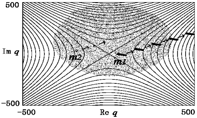
Figure 18: Iterations of small pieces of a flat manifold given by $\{(q,p)\in{\mathbb{C}}^{2}\,\,|\,\,p=p_{0}\}$ for $p_{0}=100.0+{\rm i}\,50.0$, with contour curves of the $u$ component of the $(u,v)$ coordinate superposed. One of the small pieces, $m_{1}$, is hardly deformed by the iterations of the map, and remains to be at almost the same momentum as initially given. The other one, $m_{2}$, expands over a wide range of phase space (a hatched region) after a few step iterations.

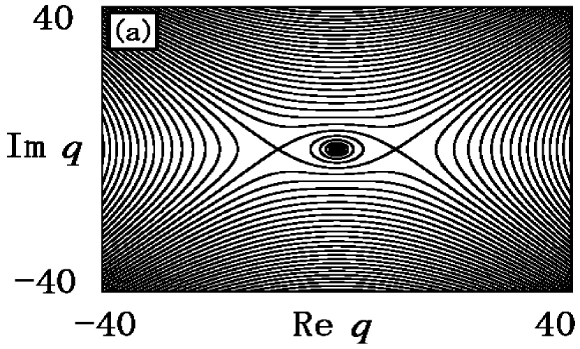
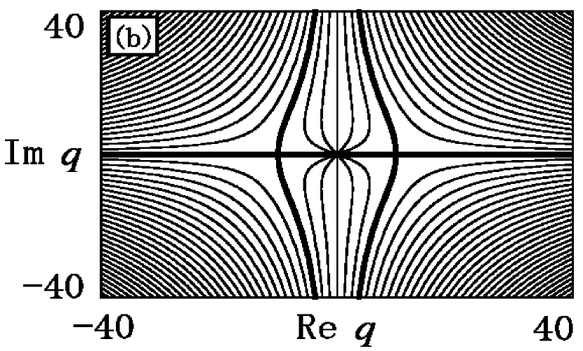
Figure 19: Contour curves of the functions (a) $A(q)$ and (b) $B(q)$. In (a), each curve is given by $A(q)=\left\{1+\log(2\gamma)\right\}/2+0.4n$ for $n\in{\mathbb{Z}}$, which approaches the axes $\hbox{Re}\,q=\pm\hbox{Im}\,q$ in both directions of the curve. In (b), each curve is given by $B(q)=\pi n/6$ for $n\in{\mathbb{Z}}$ with the branch $-\pi\leq\hbox{Arg}\,q<\pi$. Bold curves in the side of $\hbox{Re}\,q>0$ correspond to the case of $B(q)=0$, and those in the other side corresponds to the cases of $B(q)=-\pi\,(\hbox{Im}\,q\geq 0)$ and $\pi\,(\hbox{Im}\,q\leq 0)$. The bold curves intersect the real axis at $q=\pm 1/\sqrt{2\gamma}$.

Around the origin $(0,0)$, as shown in Fig. 20, the locations of the boundaries can be estimated by the single-step backward iterations of flat manifolds evaluated in real phase space. The dotted lines represent a set of folding points of the folded manifolds, each point of which is defined by the condition $dp(q)/dq=0$ where the differentiation is along each folded manifold. The set of such folding points are given by the single-step backward iterations of the lines $\{(q,p)\in{\mathbb{R}}^{2}\,|\,q=\pm 1/\sqrt{2\gamma}\}$, so that the boundaries of the partition in complex domain are expected to intersect the real domain around these lines.

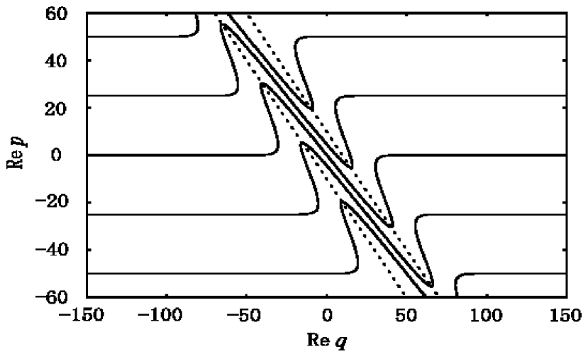
Figure 20: Single-step backward iterations of flat manifolds given by $\{(q,p)\in{\mathbb{C}}^{2}\,\,|\,\,p=p_{0}\}$ ranging from $p_{0}=-75.0$ to 75.0 by every 25.0. The dotted lines represent a set of points each of which gives the maximal or minimal momentum on each folded manifold.

We propose a partition of phase space which satisfies the rough estimations presented above both in complex and real domains. To define the partition, we prepare the notations:

$$U(x,y) = \{(q,p)\in{\mathbb{C}}^{2}\,|\,x\,\hbox{Re}\,q>0,\,\,y\,\hbox{Im}\,q>0\},\ \ \ \$$ (41a)

$$\beta(x,y,\nu) = \left[2\nu xy-(3x+1)y/2\right]\pi,$$ (41b)

where $(x,y,\nu)$ is an element of ${\cal T}\otimes{\mathbb{N}}$ which appeared in (24b). $U(x,y)$ covers a single quadrant of the $q$ plane and $\beta(x,y,\nu)$ always takes an integer times $\pi$. For $(x,y,\nu)\in{\cal T}\otimes{\mathbb{N}}$, a phase space component $U(x,y,\nu)$ is defined by

$$U(x,y,\nu) = \{(q,p)\,\,|\,\,(q,p)\in U(x,y),$$

$$\left[B(q)-\beta(x,y,\nu)\right]\left[B(q)-\beta(x,y,\nu+1)\right]\leq 0\},$$

and for $(x,y,\nu)=(0,0,0)$, by

$$U(x,y,\nu) = {\mathbb{C}}^{2}-\bigcup_{(x^{\prime},y^{\prime},\nu^{\prime})\in{\cal T}\otimes\hbox{\scriptsize\bf N}}U(x^{\prime},y^{\prime},\nu^{\prime}).$$ (43)

Then our partition ${\cal P}$ is defined as a set of the above phase space components, as already shown in (24a), and the boundaries of ${\cal P}$ take the form in (22). Such definition of partition satisfies our rough estimation for the locations of the boundaries. In fact, in the complex domain far from the origin $(0,0)$, due to (40), the relation $B(q)=\beta(x,y,\nu)$ leads to $v\approx v_{0}+n\pi/\gamma$ when we set $v_{0}=-(3x+1)y\pi/4\gamma$ and $n=\nu xy$. Moreover, Fig. 19(b) shows that the boundaries of ${\cal P}$ indicated by $B(q)=\beta(x,y,\nu)$ for $(x,y,\nu)=(1,1,1),(1,-1,1),(-1,1,1,)$ and $(-1,-1,1)$ intersect the real phase space at $q=\pm 1/\sqrt{2\gamma}$.

III.2 Properties of Homoclinic Orbits

By the partition constructed above, each homoclinic points is encoded into a sequence of symbols of the form $(x,y,\nu)$. In order to estimate imaginary parts of actions gained by homoclinic orbits, it is necessary to understand typical behaviors exhibited by the homoclinic orbits. Here we present such typical behaviors as two observations obtained from numerical computations. The first observation is concerned with the relation between the integer $\nu$, which is a member of a symbol $(x,y,\nu)$ in a symbolic sequence, and the flipping amplitude of the corresponding trajectory. The other of them is concerned with the relation between the length of a consecutive part $b\,\,b\ldots b\,\,(b\in{\cal S})$ in a symbolic sequence and the behavior of the corresponding trajectory. These are numerical observations and we have no mathematical proof, but the phase-space itinerary of any homoclinic orbit can be well explained by the combinations of the behaviors presented in these observations.

Before presenting the observations, we see the single-step folding process of flat manifolds to estimate the locations of homoclinic points in phase space. Let $m_{i}$ and $m_{f}$ be two-dimensional flat manifolds defined by the conditions $p=p_{i}$ and $p=p_{f}$ respectively, with $p_{i}$ and $p_{f}$ being complex values. The intersection $f(m_{i})\cap m_{f}$ is given by $\{(q,p_{f})\in{\mathbb{C}}^{2}\,|\,A(q)=-\log|c|,\,\,B(q)=-\arg c\pm 2\nu\pi,\,\,\nu=0,1,2,\ldots\}$ where $A(q)$ and $B(q)$ are the functions given in (40), and $c=(p_{f}-p_{i})/(2\gamma k)$. Since the $q$ components of the intersection points on $m_{f}$ are located on a single contour curve of $A(q)$, they are located along the axes $\hbox{Re}\,q=\pm\hbox{Im}\,q$ asymptotically as $\nu\rightarrow+\infty$. Also the $q$ components of homoclinic points are located along these axes asymptotically as $\nu\rightarrow+\infty$, where $\nu$ is a member of a symbol $(x,y,\nu)$ in a symbolic sequence.

Observation 1. Let $\{w_{1},w_{2},w_{3},\ldots\}$ be a set of homoclinic points whose symbolic sequences take the forms:

$$\ldots a_{-2}\,\,a_{-1}\,\,.\,\,b_{1}\,\,\,a_{1}\,\,\,a_{2}\ldots\quad\hbox{for}\,\,w_{1},$$

$$\ldots a_{-2}\,\,a_{-1}\,\,.\,\,b_{2}\,\,\,a_{1}\,\,\,a_{2}\ldots\quad\hbox{for}\,\,w_{2},$$

$$\ldots a_{-2}\,\,a_{-1}\,\,.\,\,b_{3}\,\,\,a_{1}\,\,\,a_{2}\ldots\quad\hbox{for}\,\,w_{3},$$

$$\qquad\qquad\qquad\vdots$$ (44)

where $a_{k}\,(k\neq 0)$ is any member of ${\cal S}$ defined in (24), and $b_{\nu}=(x,y,\nu)$ for $\nu=1,2,3,\ldots$ with $(x,y)\,(\in{\cal T})$ being fixed. Then the following relations hold:

$$\lim_{\nu\rightarrow+\infty}\sqrt{\gamma/(\nu\pi)}\,\,q_{0}(w_{\nu})\quad = \quad(x,y),$$ (45a)

$$\lim_{\nu\rightarrow+\infty}\sqrt{\gamma/(\nu\pi)}\,\,p_{0}(w_{\nu})\quad = \,\,-(x,y),$$ (45b)

$$\lim_{\nu\rightarrow+\infty}\sqrt{\gamma/(\nu\pi)}\,\,p_{-1}(w_{\nu})\,\, = \quad(x,y),$$ (45c)

where $(q_{0},\,p_{0})$ is the current location of $w_{\nu}$ in phase space, and $p_{-1}$ is the momentum at the last time step. The r.h.s. of each equation denotes a pair of signs of real and imaginary parts.

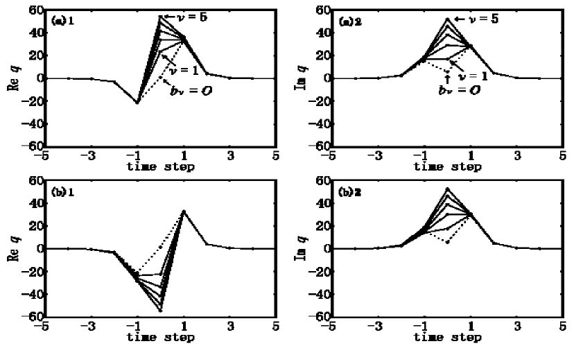
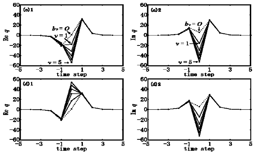
Figure 21: The trajectories of homoclinic points $w_{\nu}$ for $\nu=1,2,\ldots,5$. The left and right columns display the real and imaginary parts of the trajectories respectively. The symbolic sequence of $w_{\nu}$ is given by $\ldots O\,O\,(-1,1,1)\,.\,\,b_{\nu}\,\,(1,1,2)\,O\,O\,O\ldots$ with $b_{\nu}$ being (a) $(1,1,\nu)$, (b) $(-1,1,\nu)$, (c) $(-1,-1,\nu)$, and (d) $(1,-1,\nu)$. The dotted lines represent the case that $b_{\nu}=O$.

Fig. 21 shows the trajectories of $w_{\nu}$’s for $\nu=1,2,\ldots,5$. In these figures, one can see two facts: one is that the signs of $\hbox{Re}\,q_{0}(w_{\nu})$ and $\hbox{Im}\,q_{0}(w_{\nu})$ are described respectively by $x$ and $y$ in the symbol $b_{\nu}$. The other is that the amplitudes of $\hbox{Re}\,q_{0}(w_{\nu})$ and $\hbox{Im}\,q_{0}(w_{\nu})$ increase with $\nu$ much faster than the amplitudes at the other time steps. Due to the second fact, the following approximations hold for large $\nu$’s:

$$p_{0}\,\,\,\, = q_{1}-q_{0}\,\,\,\,\approx-q_{0},$$ (46a)

$$p_{-1} = q_{0}-q_{-1}\approx\,\,\,\,q_{0},$$ (46b)

so that the sign of $\hbox{Re}\,p_{0}(w_{\nu})$ (resp. $\hbox{Im}\,p_{0}(w_{\nu})$) is opposite to that of $\hbox{Re}\,p_{-1}(w_{\nu})$ (resp. $\hbox{Im}\,p_{-1}(w_{\nu})$) for large $\nu$’s. Fig. 22 shows $q_{0}(w_{\nu})$, $\,p_{0}(w_{\nu})$, and $p_{-1}(w_{\nu})$ for much larger $\nu$’s. The magnitudes of the real and imaginary parts of these quantities are shown to have the dependence of the form $\sqrt{\nu\pi/\gamma}$ for sufficiently large $\nu$’s. Fig. 23 shows that $q_{0}(w_{j})$ diverges much faster than $q_{-1}(w_{j})$ and $q_{-2}(w_{j})$. Similarly , $q_{0}(w_{j})$ diverges much faster than $q_{k}(w_{j})$ for any other $k\neq 0$, though that is not displayed here.

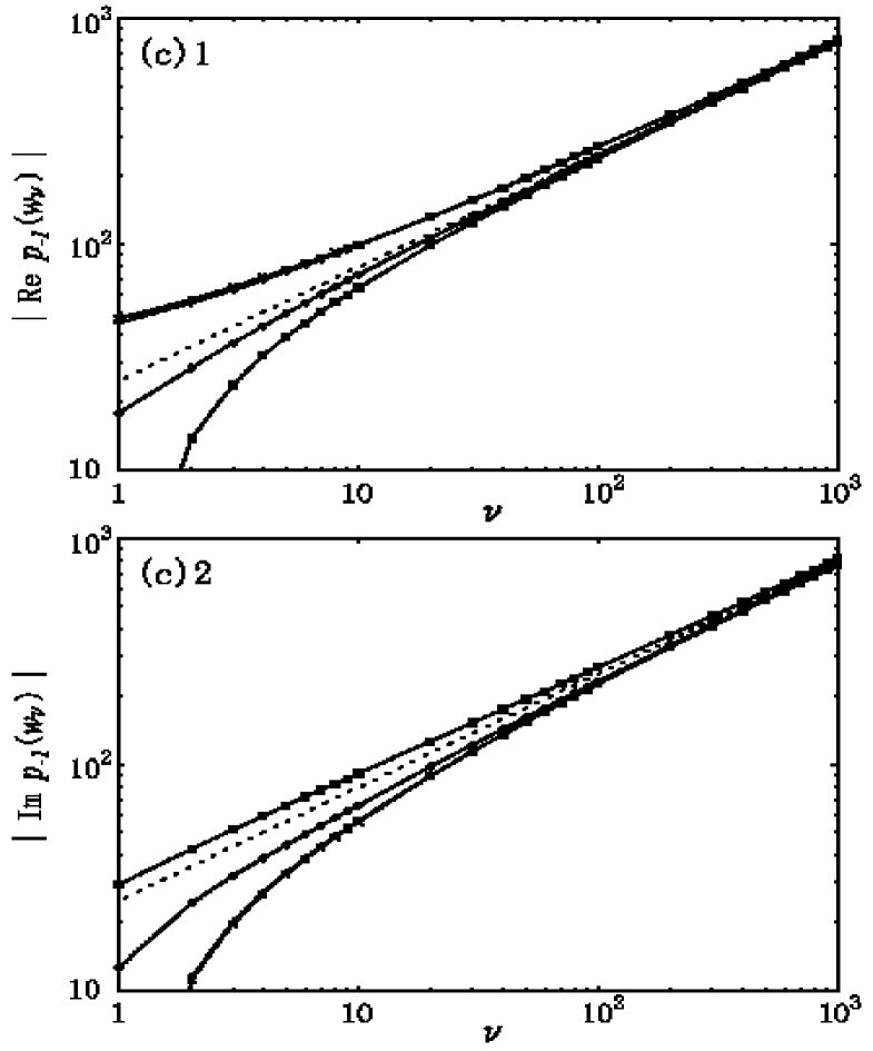
Figure 22: The dependences of (a) $q_{0}(w_{\nu})$, (b) $p_{0}(w_{\nu})$, and (c) $p_{-1}(w_{\nu})$ on the subscript number $\nu$. The symbolic sequences of $w_{\nu}$ are given in (a), where $A_{\nu},B_{\nu},$ and $C_{\nu}$ denote $(1,1,\nu),(-1,1,\nu)$, and $(-1,-1,\nu)$ respectively. The dotted line in each figure represents $\sqrt{\nu\pi/\gamma}$. In (a), all curves almost coincide.

The relation (45a) leads to

$$\lim_{\nu\rightarrow+\infty}|\hbox{Re}\,q_{0}(w_{\nu})/\hbox{Im}\,q_{0}(w_{\nu})|=1.$$ (47)

In the following, we explain why the relations (45) should follow, assuming that the relation (47) holds for the homoclinic points $w_{\nu}\,(\nu=1,2,3,\ldots)$ given by (III.2), and that $q_{0}(w_{\nu})$ diverges much faster than $q_{k}(w_{\nu})$ for any $k\neq 0$ as $\nu\rightarrow+\infty$.

The relation (45a) is explained as follows. Since $b_{\nu}=(x,y,\nu)$, $w_{\nu}$ is included in a phase space component $U(x,y,\nu)$ defined in (LABEL:def_of_phase_space_component_a) and (43). Then the $v$ component of $q_{0}(w_{\nu})$ in the $(u,v)$ coordinate diverges as $\nu\rightarrow+\infty$, since $B(q_{0}(w_{\nu}))$ diverges as $\nu\rightarrow+\infty$ due to (22), and $v\approx B(q_{0}(w_{\nu}))/(2\gamma)\approx 2\nu xy\pi/(2\gamma)$ for large $\nu$’s due to (40) and (22). Therefore from (47) and the relation $\hbox{Re}\,q_{0}\cdot\hbox{Im}\,q_{0}=v\approx\nu xy\pi/\gamma$, we obtain $q_{0}(w_{\nu})\approx\sqrt{\nu\pi/\gamma}\,(x,y)$ for large $\nu$’s.

The relation (45b) is explained as follows. The classical equations of motions in (2) lead to the relation:

$$q_{0}(w_{\nu})+q_{-2}(w_{\nu}) = 2q_{-1}(w_{\nu})-V^{\prime}(q_{-1}(w_{\nu})).$$ (48)

Since $q_{0}(w_{\nu})$ diverges much faster than $q_{-2}(w_{\nu})$ as $\nu\rightarrow+\infty$ due to our assumption, the r.h.s. of the above relation diverges in this limit. It means that $q_{-1}(w_{\nu})$ also diverges as $\nu\rightarrow+\infty$, since the r.h.s. of the relation is an entire function of $q_{-1}$. In particular, the $u$ component of $q_{-1}(w_{\nu})$ diverges as $\nu\rightarrow+\infty$, since $(q_{-1}(w_{\nu}),p_{-1}(w_{\nu}))$ is always included in the phase-space component $U(a_{-1})$ irrespective of $\nu$. Furthermore, the $u$ component diverges to $-\infty$, since if the $u$ component diverges to $+\infty$ with $(q_{-1}(w_{\nu}),p_{-1}(w_{\nu}))$ being in the same phase-space component, then $q_{-1}(w_{\nu})$ approaches the real axis and $V^{\prime}(q_{-1}(w_{\nu}))$ vanishes, so that $\hbox{Im}\left[q_{0}(w_{\nu})+q_{-2}(w_{\nu})\right]=\hbox{Im}\left[2q_{-1}(w_{\nu})-V^{\prime}(q_{-1}(w_{\nu}))\right]\rightarrow 0$. However, the above contradicts that as $\nu\rightarrow+\infty$, $\left|\hbox{Im}\left[q_{0}(w_{\nu})+q_{-2}(w_{\nu})\right]\right|\approx|\hbox{Im}\,q_{0}(w_{\nu})|\approx\sqrt{\nu\pi/\gamma}\rightarrow+\infty$. Thus the $u$ component of $q_{-1}(w_{\nu})$ diverges to $-\infty$ as $\nu\rightarrow+\infty$. When the $u$ component of $q_{-1}(w_{\nu})$ is negatively large, $V^{\prime}(q_{-1}(w_{\nu}))$ is exponentially larger than $q_{-1}(w_{\nu})$, so that $q_{0}(w_{\nu})\approx-V^{\prime}(q_{-1}(w_{\nu}))$. This relation means that $|q_{-1}|\approx\sqrt{{\gamma}^{-1}\log|q_{0}|}$, and thus $p_{0}(w_{\nu})$ has the same dependence as $q_{0}(w_{\nu})$ on $\nu$ due to the relation $p_{0}=q_{0}-q_{-1}$. The relation (45c) is explained in a similar way.

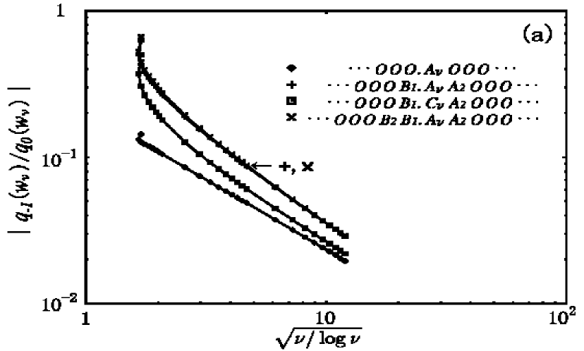
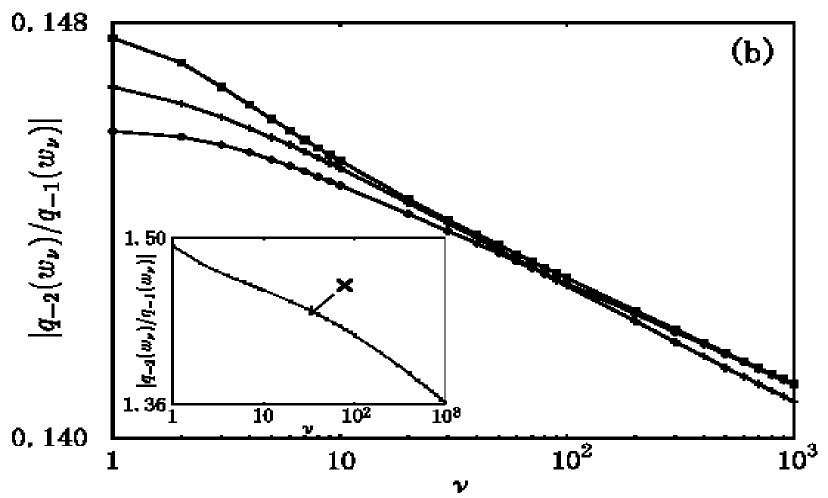
Figure 23: The $\nu$ dependence of (a) $|q_{-1}(w_{\nu})/q_{0}(w_{\nu})|$ and (b) $|q_{-2}(w_{\nu})/q_{-1}(w_{\nu})|$ (the vertical axes of (b) and the inset have the common logarithmic scale). The symbolic sequences of $w_{\nu}$ are the same as in Fig. 22. Solid lines are the guides for the eye.

We proceed to the other observation. In usual symbolic dynamics, a consecutive part $b\,\,b\ldots b$ of a single symbol $b$ in a symbolic sequence always corresponds to a fixed point in phase space or the motion approaching the fixed point. However, our classical dynamics always has only a single fixed point $(0,0)$ for any choice of positive parameters $k$ and $\gamma$, which is easily checked by solving $f(q,p)=(q,p)$, so that the phase-space motion corresponding to a consecutive part $b\,\,b\ldots b$ with $b\neq(0,0,0)$ is not obvious. Our second observation says that the phase-space motion corresponding to the above consecutive part has a turning point. It is conjectured that as the length of $b\,\,b\ldots b$ increases, the location of the turning point diverges, so that the trajectory corresponding to $b\,\,b\ldots b$ does not approach to any point in phase space in the limit of the length.

Observation 2. Let $\left\{\,w_{1},w_{2},w_{3}\ldots\right\}$ be a set of homoclinic points such that the symbolic sequences take the forms:

$$\ldots a_{-2}\,\,a_{-1}\,\,.\,\,b\,\,\,\,\,b\,\,\,\,a_{0}\,\,a_{1}\,\,a_{2}\ldots\qquad\qquad\qquad\,\,\hbox{for}\,\,w_{1},$$

$$\ldots a_{-2}\,\,a_{-1}\,\,.\,\,b\,\,\,\,\,b\,\,\,\,\,b\,\,\,\,\,b\,\,\,\,\,a_{0}\,\,a_{1}\,\,a_{2}\ldots\qquad\quad\,\,\,\,\hbox{for}\,\,w_{2},$$

$$\ldots a_{-2}\,\,a_{-1}\,\,.\,\,b\,\,\,\,\,b\,\,\,\,\,b\,\,\,\,\,b\,\,\,\,\,\,b\,\,\,\,\,b\,\,\,\,\,a_{0}\,\,a_{1}\,\,a_{2}\ldots\quad\hbox{for}\,\,w_{3},$$

$$\qquad\qquad\qquad\vdots$$ (49)

where $b\neq(0,0,0)$ and the length of $b\,\,b\ldots b$ for $w_{j}\,(j=1,2,3,\ldots)$ is $2j$. Then the trajectory of $w_{j}$ corresponding to the consecutive part $b\,\,b\ldots b$ is included in a single phase-space component $U(b)$, and the momentum almost vanishes at time step $j-1$. Moreover, the following inequalities hold:

$$0<\hbox{Re}\,q_{k-1}(w_{j})/\hbox{Re}\,q_{k}(w_{j})<1\quad(0<k<\,\,\,j),\ \ \ \ \ \$$ (50a)

$$0<\hbox{Im}\,q_{k}(w_{j})/\hbox{Im}\,q_{k-1}(w_{j})<1\quad(0<k<\,\,\,j),\ \ \ \ \ \$$ (50b)

$$0<\hbox{Re}\,q_{k}(w_{j})/\hbox{Re}\,q_{k-1}(w_{j})<1\quad(j<k<2j),\ \ \ \ \ \$$ (50c)

$$0<\hbox{Im}\,q_{k-1}(w_{j})/\hbox{Im}\,q_{k}(w_{j})<1\quad(j<k<2j).\ \ \ \ \ \$$ (50d)

This observation is exemplified in Fig. 24. In the case that the length of $\,b\,\,b\ldots b\,$ in (III.2) is given by $2j+1$ for $w_{j}$, (50a) and (50b) hold in the range of $0<k\leq j$, and (50c) and (50d) hold in the range of $j<k\leq 2j$. In this case, the momentum $p_{k}(w_{j})$ at $k=j$ is quite small, but does not vanish.

We conjecture that the $q$ component of the turning point, $q_{j}(w_{j})$, diverges with the length of $b\,\,b\ldots b$, i.e., the following relation holds:

$$\lim_{j\rightarrow+\infty}q_{j}(w_{j})=(x\!\cdot\!\infty,\,\,0),$$ (51)

where $x$ is the sign of the infinity, which is given by the member of the symbol $b=(x,y,\nu)$. This conjecture is based on the following observation.

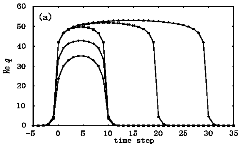
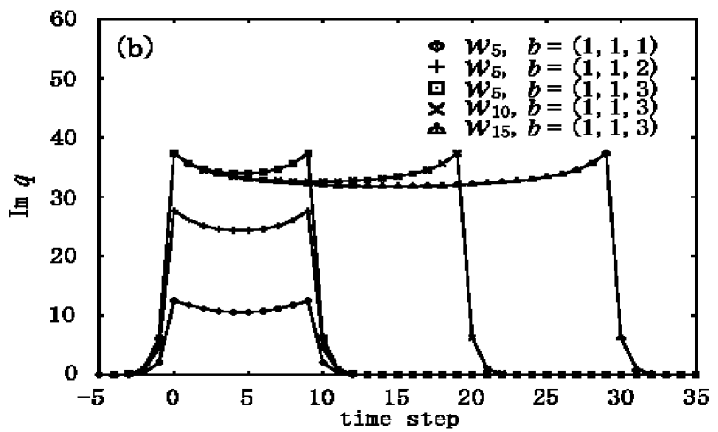
Figure 24: (a), (b) Trajectories of $w_{j}$’s for $j=$ 5, 10, and 15. The real and imaginary parts of the trajectories are displayed in (a) and (b) respectively. The symbolic sequence of $w_{j}$ is given by $\ldots\,\,O\,\,O\,.\,\,b\,\,b\,\ldots\,b\,\,O\,\,O\,\,\ldots$, where the symbol $b$ is given in (b) and the length of $b\,\,b\ldots b$ is $2j$. The real and imaginary parts of each trajectory have the maximal and minimal amplitudes respectively, at time steps $j-1$ and $j$. That is, the momentum almost vanishes at time step $j-1$. (c) Trajectories of $w_{j}$’s with the same symbolic sequences as in (a) and (b) but for $j=100$ and $b=(1,1,\nu)$ with $\nu=1,2,3$. The vector field of $V^{\prime}(q)$ is superposed with the length normalized. In (a),(b), and (c), solid lines connecting points of trajectories are the guides for the eye.

Figure 25: (a) The locations of the turning points, $q_{j}(w_{j})$, for the trajectories of $w_{j}$’s ranging from $j=1$ to 100. The symbolic sequences of $w_{j}$’s are the same as is given in the caption of Fig. 24. (b) The magnitude and phase of the potential function $V(q)$ at the turning point $q_{j}(w_{j})$ for ranging from $j=1$ to 100. The phase, $-2\gamma\hbox{Re}\,q_{j}\cdot\hbox{Im}\,q_{j}$, is plotted without taking mod $2\pi$. In (a) and (b), solid lines are the guides for the eye.

Fig. 25 shows the locations of the turning points $q_{j}(w_{j})$ ranging from $j=1$ to 100, and the magnitudes and phases of the potential function $V(q)$ at the turning points. It can be seen that as $j$ increases, the magnitude of $V(q_{j}(w_{j}))$ decreases to zero algebraically, and the phase of $V(q_{j}(w_{j}))$ approaches some constant. That is, $V(q_{j}(w_{j}))\approx\alpha j^{-\beta}e^{{\rm i}\theta}$ for large $j$’s, where $\alpha,\beta$ (both positive), and $\theta$ depend on a symbol $b$ which consists of a consecutive part $b\,b\ldots b$ in a symbolic sequence of $w_{j}$. If this approximation holds for any large $j$, solving the equation $V(q_{j}(w_{j}))=\alpha j^{-\beta}e^{{\rm i}\theta}$, one obtains the solution:

$$u_{j}(w_{j}) = \left[\beta\log j-\log(\alpha/k)\right]/(2\gamma),$$ (52a)

$$v_{j}(w_{j}) = -\theta/(2\gamma),$$ (52b)

where $(u_{j}(w_{j}),v_{j}(w_{j}))$ is the location of $q_{j}(w_{j})$ on the $(u,v)$ coordinate defined in (39). This solution suggests that $\hbox{Re}\,q_{j}(w_{j})$ diverges and $\hbox{Im}\,q_{j}(w_{j})$ vanishes as $j\rightarrow+\infty$. Moreover, according to the Observation 2, $q_{j}(w_{j})$ and the $q$ component of $U(b)$ are included in the same quadrant of the $q$ plane. Therefore the relation (51) is obtained. The justification of this relation needs further investigation of classical dynamics, and we hope to report the result of this issue elsewhere.

We have shown that there are two types of behaviors exhibited by homoclinic orbits. In our numerical computations, the behavior of any homoclinic orbits can be understood by the combinations of only two types of motions, one of which is the flipping motions almost along the axes $\hbox{Re}\,q=\pm\hbox{Im}\,q$, and the other of which is the motions almost along the contour curves of the $v$ component in the $(u,v)$ coordinate. Which type of motion occurs in the process from $(q_{k},p_{k})$ to $(q_{k+1},p_{k+1})$ along a single homoclinic trajectory depends on whether the neighbouring symbols in a symbolic sequence, $a_{k}$ and $a_{k+1}$, are the same (the latter type) or not (the former type). The former type of motion is characterized by the Observation 1, and the latter one by the Observation 2.

III.3 Estimation of Imaginary Parts of Actions

The imaginary parts of actions gained by the orbits of homoclinic points are estimated from the symbolic sequences assigned to the points. We first consider the homoclinic points appearing in the Observations 1 and 2, and the estimations of imaginary parts of actions for these cases are presented as the Observations 3 and 4 respectively. Then using the latter two observations, we estimate the imaginary part of action for any homoclinic trajectory. The Observation 3 says that the imaginary part of action diverges linearly as $\nu\rightarrow+\infty$, where $\nu$ is a member of a symbol $(x,y,\nu)$ in a symbolic sequence. The Observation 4 says that the amount of the imaginary part of action is bounded even if the length of a consecutive part $b\,\,b\ldots b\,\,(b\in{\cal S})$ in a symbolic sequence tends to infinity. In particular, we observed that the itinerary described by $b\,\,b\ldots b$ gains little imaginary part of action compared to the other itineraries in a trajectory. This means that the homoclinic orbits appearing in the Observation 4 can play a semiclassically significant role. The Observations 3 and 4 are also entirely based on our numerical computations, and so far, we have no mathematical proof for these observations.

For the trajectory of any homoclinic point $w$, here we consider the following imaginary part of action:

$$s(w) = \sum_{k=1}^{+\infty}\hbox{Im}\left[T(p_{k-1}(w))-V(q_{k}(w))\right],$$ (53)

where $(q_{k}(w),p_{k}(w))$ denotes the $k$ step iteration of $w$. The sum in the r.h.s. converges due to the exponential convergence of the trajectory to the origin $(0,0)$, and it is the long-time limit of $\hbox{Im}\,S_{n}$ which is given in (8c). In the definition of $s(w)$, we only take account of the contributions from the forward trajectories, since semiclassical wave functions in the time domain are determined by them. We do not define $s(w)$ as the long-time limit of $\hbox{Im}\,{\tilde{S}}_{n}$ which is given in (8b), since it includes an additional term $S_{0}$ which depends only on the choice of an incident wave packet, not on classical dynamics. First we estimate $s(w)$ for the homoclinic points appearing in the Observation 1.

Observation 3. Let $\left\{w_{1},w_{2},w_{3},\ldots\right\}$ be a set of homoclinic points which appears in the Observation 1. Then for any integer $n\geq 1$, the following relation holds:

$$\lim_{\nu\rightarrow+\infty}\left[\gamma/(2\nu\pi)\right]s(f^{-n}(w_{\nu})) = xy.$$ (54)

Fig. 26(a) shows the magnitudes of $s(f^{-n}(w_{j}))$ for $n=4$ and $\nu=1$ to $1000$. It can be seen that $|s(f^{-n}(w_{\nu}))|\approx 2\nu\pi/\gamma$ for large $\nu$’s. The condition $n\geq 1$ in (54) is imposed to always take account of the contributions from the flipping motions from $q_{-1}(w_{\nu})$ to $q_{0}(w_{\nu})$ displayed in Fig. 21.

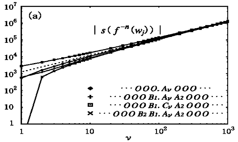
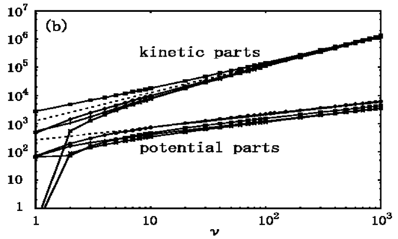
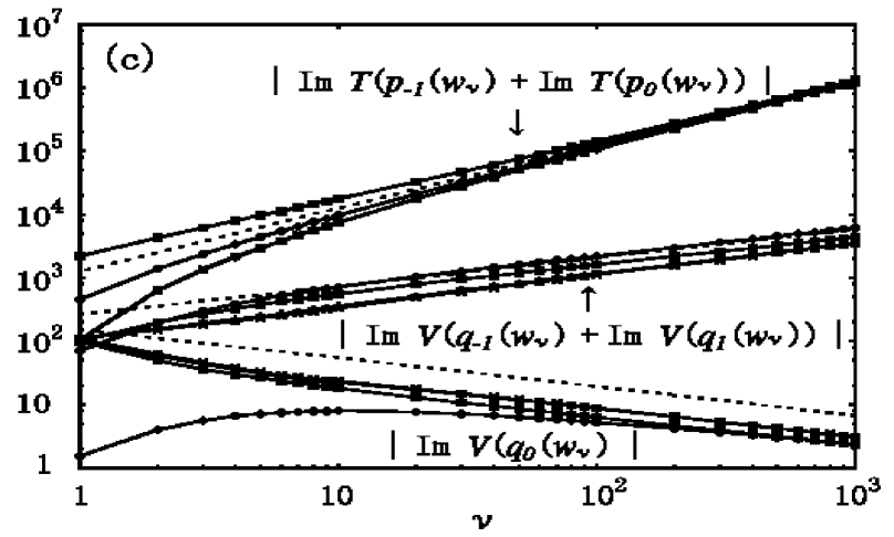
Figure 26: (a) The absolute values of the imaginary parts of actions, $|s(f^{-n}(w_{\nu}))|$, for $n=4$ and $\nu=1$ to $1000$. The symbolic sequences of $w_{\nu}$’s are the same as in Fig. 22. The dotted line represents $2\nu\pi/\gamma$. (b) The absolute values of the kinetic parts and the potential ones of $s(f^{-n}(w_{\nu}))$. The upper dotted line and the lower dotted curve represent $2\nu\pi$ and $2f(\sqrt{2\nu\pi/\gamma})$ respectively, where $f(x)=x/(2\sqrt{\gamma\log x})$. (c) $|\hbox{Im}\,T(p_{-1}(w_{\nu}))+\hbox{Im}\,T(p_{0}(w_{\nu}))|$, $|\hbox{Im}\,V(q_{-1}(w_{\nu}))+\hbox{Im}\,V(q_{1}(w_{\nu}))|$, and $|\hbox{Im}\,V(q_{0}(w_{\nu}))|$. The top dotted line and middle dotted curve are the same as in (b), and the bottom dotted curve represents $\{2\gamma^{2}f(\sqrt{2\nu\pi/\gamma})\}^{-1}$. In each figure, the solid lines are guides for the eye.

In the following, we explain the relation (54), assuming that the Observation 1 holds, and that for the homoclinic points appearing in the Observation 1, $q_{k}(w_{\nu})$ (resp. $q_{-k}(w_{\nu})$) for $k=0,1,2,\ldots$ diverges much faster than $q_{k+1}(w_{\nu})$ (resp. $q_{-(k+1)}(w_{\nu})$) as $\nu\rightarrow+\infty$. Fig. 23 suggests that the second assumption is valid for $k=0$ and $1$. For the other $k$’s, it has not been found numerically whether the assumption is valid or not, since $q_{k}(w_{\nu})$ and $q_{-k}(w_{\nu})$ for $k\geq 2$ remain to be immediate values even for $\nu\approx 1000$, so that the numerical computation needs too high accuracy to make clear the asymptotic behaviors of $|q_{k}|$ and $|q_{-k}|$ with sufficiently large magnitudes. However, the exponential dependence of $V^{\prime}(q)$ on $u$ and $v$ shown in (40) means that the large difference in $q_{k}(w_{j})$ (resp. $q_{-k)}(w_{j})$) results from the slight difference in $q_{k+1}(w_{j})$ (resp. $q_{-(k+1)}(w_{j})$) by the map $f^{-1}$ (resp. $f$), so that the assumption for $k\geq 2$ is expected to be valid.

The relation (54) is explained as follows. In the kinetic part of $s(f^{-n}(w_{\nu}))$, i.e., $\Sigma_{k=-n+1}^{+\infty}\hbox{Im}\,T(p_{k-1}(w_{\nu}))$, each term is written as

$$\hbox{Im}\,T(p_{k-1}(w_{\nu})) = \left[\hbox{Re}\,p_{k-1}(w_{\nu})\right]\left[\hbox{Im}\,p_{k-1}(w_{\nu})\right].\ \ \ \$$ (55)

Due to the assumptions we put, the following inequalities hold for $k\neq 0,-1$ and for large $\nu$’s:

$$|\hbox{Re}\,p_{k}(w_{\nu})| \ll |\hbox{Re}\,p_{-1}(w_{\nu})|,|\hbox{Re}\,p_{0}(w_{\nu})|,$$ (56a)

$$|\hbox{Im}\,p_{k}(w_{\nu})| \ll |\hbox{Im}\,p_{-1}(w_{\nu})|,|\hbox{Im}\,p_{0}(w_{\nu})|.$$ (56b)

Then the kinetic part of $s(f^{-n}(w_{\nu}))$ is dominated by the terms $\hbox{Im}\,T(p_{-1}(w_{\nu}))$ and $\hbox{Im}\,T(p_{0}(w_{\nu}))$ due to (55). Since the Observation 1 says that the quantities in the r.h.s. of the above inequalities have ${\nu}^{1/2}$ dependences on large $\nu$’s, $\hbox{Im}\,T(p_{-1}(w_{\nu}))$ and $\hbox{Im}\,T(p_{0}(w_{\nu}))$ have linear dependences on large $\nu$’s due to (55). Therefore the kinetic part of $s(f^{-n}(w_{\nu}))$ is expected to has a linear dependence on large $\nu$’s. Fig. 26 shows that the kinetic part of $s(f^{-n}(w_{\nu}))$ is actually dominated by $\hbox{Im}\,T(p_{-1}(w_{\nu}))$ and $\hbox{Im}\,T(p_{0}(w_{\nu}))$, and has a linear dependence on large $\nu$’s.

In the potential part of $s(f^{-n}(w_{\nu}))$, i.e., $\Sigma_{k=-n+1}^{+\infty}\hbox{Im}\,V(q_{k}(w_{\nu}))$, each term is written as

$$\hbox{Im}\,V(q_{k}(w_{\nu})) = \hbox{Im}\left[\frac{q_{k+1}(w_{\nu})-2q_{k}(w_{\nu})+q_{k-1}(w_{\nu})}{2\gamma q_{k}(w_{\nu})}\right],$$

by incorporating the classical equations of motions given in (2) with the relation $V^{\prime}(q)=-2\gamma qV(q)$ satisfied by our potential function. A simple calculation of the r.h.s. of (LABEL:special_relation_of_V) yields an inequality:

$$|\hbox{Im}\,V(q_{k}(w_{\nu}))| \leq \frac{|q_{k+1}(w_{\nu})|+|q_{k-1}(w_{\nu})|}{2\gamma|q_{k}(w_{\nu})|}.$$ (58)

Based on the assumptions imposed here, we can present the same discussion as that below (47) (note that the assumptions here are stronger than those imposed there). As a result, one obtains the relations $|q_{1}(w_{\nu})|,|q_{-1}(w_{\nu})|\approx\sqrt{\gamma^{-1}\log|q_{0}(w_{\nu})|}$ for large $\nu$. In a similar way, one obtains the relations $|q_{\pm(k+1)}(w_{\nu})|\approx\sqrt{\gamma^{-1}\log|q_{\pm k}(w_{\nu})|}$ for large $\nu$’s and $k=1,2,3,\ldots$. By using these relations, the r.h.s. of (58) is approximated by

$$\left[2\gamma^{2}f(|q_{k}(w_{\nu})|)\right]^{-1}\quad \quad k=0,$$ for (59a)

$$f(|q_{k-1}(w_{\nu})|)\qquad \quad k>0,$$ for (59b)

$$f(|q_{k+1}(w_{\nu})|)\qquad \quad k<0,$$ for (59c)

where $f(x)=x/(2\sqrt{\gamma\log x})$. Here we used an approximation $|q|+\sqrt{\gamma^{-1}\log|q|}\approx|q|$ for large $|q|$.

Since $|q_{0}(w_{\nu})|$ is approximated as $\sqrt{2\nu\pi/\gamma}$ for large $\nu$’s according to the Observation 1, the r.h.s. of (58) is approximated by

$$\left[2\gamma^{2}f\left(\sqrt{2\nu\pi/\gamma}\right)\right]^{-1}\qquad\quad\! k=0,\ \ \ \ \ \$$ for (60a)

$$f\left(\sqrt{2\nu\pi/\gamma}\right)\qquad\qquad\! k=\pm 1,\ \ \ \ \ \$$ for (60b)

$$f\left(\sqrt{\log^{\prime}(\log^{\prime}(\ldots\log^{\prime}(\log^{\prime}(2\pi\nu/\gamma))\ldots))}\right)\, |k|\geq 2,\ \ \ \ \ \$$ for (60c)

where $\log^{\prime}x=(2\gamma)^{-1}\log x$, and the argument of the square root in (60c) is a $|k|-1$ fold logarithm of $2\pi\nu/\gamma$.

Since $f(x)$ in (60) is monotonically increasing for large $x$, one can expect that the potential part of $s(f^{-n}(w_{\nu}))$ for large $\nu$’s is dominated by the terms $\hbox{Im}\,V(q_{-1}(w_{\nu}))$ and $\hbox{Im}\,V(q_{1}(w_{\nu}))$. More precisely, from (60b), the potential part of $s(f^{n}(w_{\nu}))$ is expected to be approximated by $2f(\sqrt{2\nu\pi/\gamma})$ for large $\nu$’s. And also, from (60a), $\hbox{Im}\,V(q_{0}(w_{\nu}))$ is expected to vanish as $\nu\rightarrow+\infty$. Fig. 26 shows that the potential part of $s(f^{-n}(w_{\nu}))$ is actually dominated by the terms $\hbox{Im}\,V(q_{-1}(w_{\nu}))$ and $\hbox{Im}\,V(q_{1}(w_{\nu}))$ for large $\nu$’s, and the asymptotic behavior of the potential part for large $\nu$’s is described by $2f(\sqrt{2\nu\pi/\gamma})$. It is also shown that $\hbox{Im}\,V(q_{0}(w_{\nu}))$ tends to vanish as $\nu$ increases.

Consequently, due to the $\nu$ dependencies of kinetic and potential parts as seen above, $s(f^{-n}(w_{\nu}))$ for large $\nu$’s is dominated by the kinetic part, which has a linear dependence of large $\nu$’s. Therefore the following estimation is obtained for large $\nu$’s:

$$s(f^{-n}(w_{\nu})) \approx \hbox{Im}\,T(p_{-1}(w_{\nu}))+\hbox{Im}\,T(p_{0}(w_{\nu}))$$ (61)

$$= \hbox{Re}\,p_{-1}(w_{\nu})\cdot\hbox{Im}\,p_{-1}(w_{\nu})$$

$$+\hbox{Re}\,p_{0}(w_{\nu})\cdot\hbox{Im}\,p_{0}(w_{\nu})$$

$$\approx (2\nu\pi/\gamma)xy.$$

In the last approximation, the relations in (45) are used.

Next we estimate $s(w)$ for the homoclinic points appearing in the Observation 2.

Observation 4. Let $\left\{w_{1},w_{2},w_{3},\ldots\right\}$ be a set of homoclinic points which appears in the Observation 2. Then for any integer $n$, a sequence of imaginary parts of actions,

$$s(f^{-n}(w_{1}))\,\,\,s(f^{-n}(w_{2}))\,\,\,s(f^{-n}(w_{3}))\ldots,$$ (62)

is bounded.

Fig. 27(a) shows $s(f^{-n}(w_{j}))$ for $n=4$ and $j=1$ to 100. It can be seen that $s(f^{-n}(w_{j}))$ $(j=1,2,3,\ldots)$ does not deviate largely from $s(f^{-n}(w))$ for a homoclinic point $w$ which has a symbolic sequence:

$$\ldots O\,\,O\,.\,b\,\,\,O\,\,O\ldots.$$ (63)

In the case of Fig. 27(a), $s(f^{-n}(w_{j}))$ $(j=1,2,3,\ldots)$ is mainly gained by the flippings of trajectories between phase-space components $U(b)$ and $U(O)$ ($O=(0,0,0)$). Though not displayed here, also in the case of the symbolic sequence:

$$\ldots a_{-2}\,a_{-1}\,.\,b\,\,\,b\ldots b\,\,\,a_{0}\,\,a_{1}\ldots$$ (64)

with $\ldots a_{-2}\,a_{-1}\neq\ldots O\,\,O$ or $a_{0}\,\,a_{1}\ldots\neq O\,\,O\ldots$, the imaginary part of action does not deviate largely from that in the case of the sequence:

$$\ldots a_{-2}\,a_{-1}\,.\,b\,\,\,a_{0}\,\,a_{1}\ldots.$$ (65)

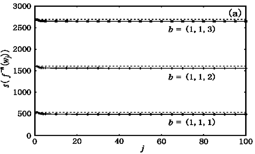
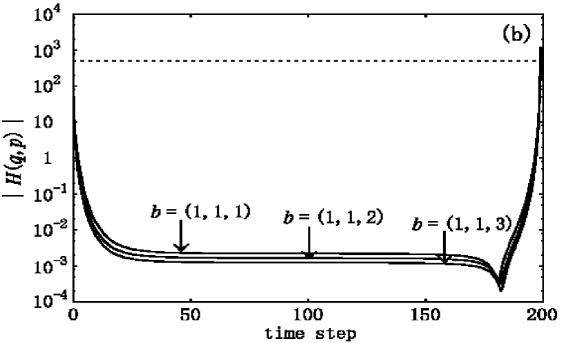
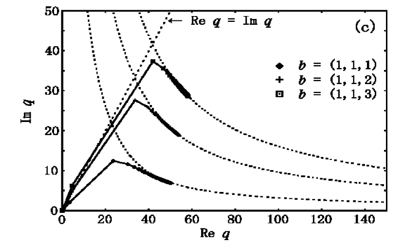
Figure 27: (a) The imaginary actions $s(f^{-n}(w_{j}))$ plotted for $n=4$ and $j=1$ to 100. In (a),(b), and (c), the symbolic sequence of $w_{j}$ is given by $\ldots O\,O\,.\,\,b\,\,b\ldots\,b\,\,O\,O\,\ldots$, where $b=(1,1,\nu)$ with $\nu=1,2,3$, and the length of $b\,\,b\ldots\,b$ is given by $2j$. The solid lines indicate the values of the imaginary parts of actions in the case that the length of $b\,\,b\ldots b$ is one. (b) The magnitudes of the Hamiltonian $H(q,p)=p^{2}/2+ke^{-\gamma q^{2}}$ (solid curves) along the forward trajectories of $w_{j}$’s for $j=100$. The dotted line represents the magnitude of the Hamiltonian at the origin $(0,0)$. (c) The homoclinic trajectories already shown in Fig. 24(c), and integrable trajectories (dotted curves) which satisfy $H(q,p)=0$ and connect two infinities of the $q$ plane, $(\hbox{Re}\,q,\hbox{Im}\,q)=(+\infty,0)$ and $(0,+\infty)$. The dotted line sprouting from the origin represents $\hbox{Re}\,q=\hbox{Im}\,q$. The solid lines are the guides for the eye.

Therefore the imaginary parts of actions are mainly gained by phase-space itineraries described by sequences other than $b\,\,b\ldots b$. This means that itineraries described by $b\,\,b\ldots b$ can be semiclassically significant in the tunneling process, since smaller imaginary parts of actions yield larger semiclassical amplitudes. As in the Observation 2, the same statement as the Observation 4 holds when the length of the sequence $b\,\,b\ldots b$ is given by $2j+1$ for a homoclinic point $w_{j}$.

We discuss why the sequence (62) is bounded. Fig. 27(c) shows the same homoclinic trajectories as in Fig. 24(c), and integrable trajectories of a Hamiltonian $H(q,p)=p^{2}/2+ke^{-\gamma q^{2}}$. The integrable trajectories are chosen so that they satisfy $H(q,p)=0$ and connect two infinities on the $q$ plane, $(\hbox{Re}\,q,\hbox{Im}\,q)=(+\infty,0)$ and $(0,+\infty)$. It can be seen that the homoclinic trajectories are along the integrable trajectories at intermediate time steps. In fact, as shown in Fig. 27(b), $H(q,p)$ for the homoclinic trajectories almost vanishes at these time steps.

The previous Fig. 25(b) implies that the potential function at the turning points, $V(q_{j}(w_{j}))$ $\left(\approx V(q_{j-1}(w_{j}))\right)$, vanishes as $j\rightarrow+\infty$. Then it is expected that even for sufficiently large $j$’s, $H(q,p)\approx 0$ when the trajectories of $w_{j}$’s are around their turning points, and that the trajectories are approximated by the integrable trajectories satisfying $H(q,p)=0$.

If the above expectation is correct, the imaginary parts of actions gained by the trajectories of $w_{j}$’s described by a sequence $b\,\,b\ldots b$ can be evaluated by the integrable trajectories. For our present parameter values $k=500$ and $\gamma=0.005$, the magnitudes of the imaginary parts of actions are estimated to be less than about 900 (see the Appendix II). This value is an over-estimated one because homoclinic trajectories and integrable ones do not agree very well around the axis $\hbox{Re}q=\hbox{Im}q$ from where the actions along integrable trajectories are integrated.

By making use of the Observations 3 and 4, we estimate the imaginary parts of actions gained by the orbits of homoclinic points from the symbolic sequences assigned to the points. Let $w$ be a homoclinic point whose symbolic sequence is given by

$$\ldots a_{-2}\,a_{-1}\,\,.\,\,a_{0}\,\,a_{1}\,\,a_{2}\ldots,$$ (66)

where $a_{k}=(x_{k},y_{k},\nu_{k})$ for $k\in{\mathbb{Z}}$. We assume that $\nu_{k}$ is large if $a_{k}\neq(0,0,0)$.

In the case that the symbolic sequence in (66) does not include a consecutive part, $b\,\,b\ldots b$, we approximate $q_{k}(w)$ for any $k\in{\mathbb{Z}}$ according to the Observation 1 by

$$q_{k}(w) \approx (\nu_{k}\pi/\gamma)^{1/2}\,\,(x_{k},y_{k}).$$ (67)

For $a_{k}=(0,0,0)$, substituting $(x_{k},y_{k})=(0,0)$ into (67), we approximate $q_{k}(w)$ by $0$. From the relation $p_{k-1}=q_{k}-q_{k-1}$, we approximate $p_{k-1}(w)$ by

$$p_{k-1}(w) \approx (\pi/\gamma)^{1/2}(x_{k}{\nu_{k}}^{1/2}-x_{k-1}{\nu_{k-1}}^{1/2},$$ (68)

$$y_{k}{\nu_{k}}^{1/2}-y_{k-1}{\nu_{k-1}}^{1/2}).$$

Then due to (55), $\hbox{Im}\,T(p_{k-1}(w))$ is approximated by

$$\hbox{Im}\,T(p_{k-1}(w)) \approx (\pi/\gamma)(x_{k}{\nu_{k}}^{1/2}-x_{k-1}{\nu_{k-1}}^{1/2})$$ (69)

$$\times(y_{k}{\nu_{k}}^{1/2}-y_{k-1}{\nu_{k-1}}^{1/2}).$$

Since the imaginary part of action gained at each time step is dominated by the kinetic part, as discussed at the Observation 3, $s(w)$ is estimated by the sum over the terms in the r.h.s. of (69) for $k\geq 1$.

In the case that the symbolic sequence in (66) includes a consecutive part, $b\,\,b\ldots b$, the imaginary part of action gained along the itinerary described by $b\,\,b\ldots b$ is negligible compared to that along the other part of the trajectory, as discussed below the Observation 4. Based on this fact, we approximate the imaginary part of action for $b\,\,b\ldots b$ by a null value. This approximation allows us to evaluate the imaginary part of action only by the kinetic part also in the case of $b\,\,b\ldots b$. It is because the r.h.s. of (69) is null when $(x_{k-1},y_{k-1},\nu_{k-1})=(x_{k},y_{k},\nu_{k})$ so that the imaginary part of action associated with $b\,\,b\ldots b$ is evaluated as a null value. As a result, whether a consecutive part $b\,\,b\ldots b$ is included in a symbolic sequence or not, the imaginary part of action is estimated only by the kinetic part of action.

Figure 28: Imaginary parts of actions evaluated from (a) actual trajectories of homoclinic points, and (b) symbolic sequences assigned to the homoclinic points. In each figure, the origin represents a null imaginary part of action gained by the trajectory of a fixed point associated with a symbolic sequence $\ldots O\,\,O\,\,.\,\,O\,\,O\,\,O\ldots\,\,\left(O=(0,0,0)\right)$. The first to the third columns labeled by $a_{1}$,   $a_{1}a_{2}$, and $a_{1}a_{2}a_{3}$ show respectively the imaginary parts of actions gained by the trajectories of the homoclinic points associated with $\ldots O\,\,O\,\,.\,\,O\,\,O\,\,O\,\,a_{1}\,\,O\,\,O\ldots$, $\ldots O\,\,O\,\,.\,\,O\,\,O\,\,O\,\,a_{1}\,\,a_{2}\,\,O\,\,O\ldots$, and $\ldots O\,\,O\,\,.\,\,O\,\,O\,\,O\,\,a_{1}\,\,a_{2}\,\,a_{3}\,\,O\,\,O\ldots$, where $a_{1},a_{2},a_{3}$ are the members of $\{(1,1,\nu)\,\,|\,\,\nu=1,2,3\}$.

Finally, for the homoclinic point $w$ whose symbolic sequence is given by (66), $s(w)$ is estimated as follows:

$$s(w) \approx \sum_{k=1}^{+\infty}\hbox{Im}\,T(p_{k-1}(w))$$

$$\approx \frac{\pi}{\gamma}\sum_{k=1}^{+\infty}(x_{k}{\nu}_{k}^{1/2}-x_{k-1}{\nu}_{k-1}^{1/2})(y_{k}{\nu}_{k}^{1/2}-y_{k-1}{\nu}_{k-1}^{1/2}).$$

Fig. 28 shows the imaginary parts of actions evaluated from actual trajectories of homoclinic points and from symbolic sequences assigned to the homoclinic points. The estimation (LABEL:derivation_of_estimation_formula) is based on the assumption that each $\nu_{k}$ is large if $a_{k}\neq(0,0,0)$, however, as shown in the figure, the estimation is still valid for small $\nu_{k}$. This is because the approximation in (67) are not so crude for small $\nu_{k}$, as is shown in Fig. 22(a).

In each column of Fig. 28(a), the smallest $s(w)$ is associated with a symbolic sequence $\ldots O\,\,O\,.\,O\,\,O\ldots$ or $\ldots O\,\,O\,.\,O\,\,O\,\,O\,\,b\,\,\,b\ldots b\,\,O\,\,O\ldots$ with $b=(1,1,1)$. The Appendix II shows such types of symbolic sequences, including the case that $b=(-1,-1,1)$, attain the smallest $s(w)$ in the whole candidates. In the previous Sec. II.6, we evaluated the tunneling wave functions by the semiclassical candidate orbits described by these types of sequences, typical behavior of which was illustrated in Fig. 15(c).

IV Conclusion and Discussion

IV.1 Conclusion

We have carried out complex semiclassical analysis for the tunneling problem of a simple scattering map which creates chaotic dynamics in complex domain. Although classical motions in real phase space are simple, Tunneling wave functions exhibit a complicated pattern, which is typically observed in chaotic systems. The wave functions were reproduced semiclassically in excellent agreement with fully quantum calculations. It enables us to interpret the creation of the complicated pattern appearing in the tunneling regime. Complex orbits contributing to the semiclassical wave function are embedded in a hierarchical structure of an initial-value set. The hierarchical structure is a reflection of the emergence of homoclinic tanglement in complex phase space, i.e., the manifestation of complex-domain chaos. On the basis of symbolic dynamics constructed in the complex domain, phase space itineraries of tunneling orbits were related with the amounts of imaginary parts of actions gained by the orbits. Incorporation of symbolic dynamics with the complex semiclassical method has enabled us to discuss quantitatively the competition among tunneling orbits, and has elucidated the significant role of complex-domain chaos in the tunneling process of non-integrable systems.

IV.2 Chaotic Tunneling

We further discuss the role of complex-domain chaos played in the semiclassical description of tunneling in non-integrable systems. In the present study, we adopted a time-domain approach of the complex semiclassical method. This approach is concerned with the real-time classical propagation, and has nothing to do with the instanton process. This means that real-domain paths are not connected to complex-domain paths, in other words, both the real domain and the other domain are invariant under the classical dynamics. Therefore all candidate orbits to describe tunneling are always exposed to complex-domain chaos, not to real-domain one. In this sense, it is natural to consider the role of the complex-domain chaos in our approach.

On our semiclassical framework, initial and final quantum states are identified with classical manifolds in complex phase space. The evolution of the manifolds is involved in the stretching and folding dynamics in the complex domain. The chain-like structure which we observed is nothing but the structure of the section of one backward evolved manifold, $f^{-n}({\cal F})$, cut by the other manifold ${\cal I}$. Our result here strongly suggests that the creation of the chain-like structure is only due to the emergence of complex-domain chaos, irrespective of the existence of real-domain chaos and also irrespective of the types of tunneling, i.e., whether energy-barrier tunneling or dynamical one ShudoIkeda2 .

The chaotic dynamics in phase space is created on the Julia set, which includes the complex homoclinic tanglement investigated here. The trajectories on this set are proven to be sufficient to describe tunneling in the case of the complex Hénon map ShudoIshiiIkeda . It was numerically confirmed here that this statement is correct also in our case. Therefore, on the basis of our present study and Ref. ShudoIshiiIkeda , we would like to present the notion of “chaotic tunneling”, which first appeared in Ref. ShudoIkeda1 , as the tunneling in the presence of the Julia set.

In energy domain approaches Frischat ; Creagh ; TakahashiYoshimotoIkeda ; Brodier , to our knowledge, the complex-domain chaos has not been used explicitly in semiclassical calculations. The significant role of the complex domain chaos played in the time domain approach should have the correspondence in the energy-domain ones. However, the instanton concept, which is intrinsic to these approaches, makes it difficult to see such correspondence. The reason is that even when one takes full account of complex classical dynamics, the degree of freedom of the path deformation on the complex time plane often allows one to consider complicated classical processes in complex domain as the composition of real-domain chaotic processes and instanton-like ones Creagh ; TakahashiYoshimotoIkeda . We would like to describe the tunneling phenomena in non-integrable systems in terms of the simple notion, chaotic tunneling. Therefore the role of complex-domain chaos in the energy domain approaches is desired to be clarified in further studies.

IV.3 Discussion

Finally, we here itemize several future problems where are necessary to make our theory more self-contained:

1. We have constructed a partition of phase space in terms of the phase part of the gradient of a potential function. A similar approach can be found in the context of the study on a dynamical system of an exponential map of one complex variable Devaney , where the boundaries of a partition correspond to the contour curves of the phase part of the exponential function. Genericness of our approach should be examined in further studies.

2. Reproducing tunneling wave functions, we did not enter into details of the treatment of the Stokes phenomenon. Empirically, symbolic sequences which include members of the form $(1,-1,\nu)$ or $(-1,1,\nu)$ with $\nu\in{\mathbb{Z}}$ should be excluded from the whole candidates. In particular, according to such empirical rule, we have excluded from the candidates those trajectories which have almost null imaginary parts of actions due to the cancellation between the imaginary parts gained at individual time steps. When the condition $q_{n+k}=q_{n-k-1}^{\ast}$ is satisfied for any $k\geq 0$ with $n$ being fixed, where the asterisk denotes the complex conjugate, the imaginary parts of actions integrated over the whole time axis become null. We observed numerically that such condition is satisfied by the symbolic sequences of homoclinic points such that the relation between symbols, $(x_{n+k},y_{n+k},\nu_{n+k})=(x_{n-k-1},-y_{n-k-1},\nu_{n-k-1})$, holds for any $k\geq 0$ with $n$ being fixed. In fact, there are an infinite number of symbolic sequences satisfying such relation. The criterion for whether tunnneling orbits well approximated by the homoclinic orbits described by such symbolic sequences are semiclassically contributable or not would be beyond our intuitive expectation based on the amount of imaginary parts of actions ShudoIkeda3 . The criterion should be given only by a rigorous treatment of the Stokes phenomenon. The justification of our empirical rule mentioned above needs the consideration of the intersection problem of the Stokes curves, and we are now investigating this issue OnishiShudo .

3. In many non-integrable open systems with the condition that $V^{\prime}(q)\rightarrow 0$ as $|q|\rightarrow+\infty$, real-domain trajectories which diverge to infinity are indifferent, i.e., have null Lyapunov exponents, in contrast to the case of open systems with polynomial potential functions. Because of that, in the former systems, generaic properties of complex trajectories exploring in the vicinity of real-domain asymptotic region are not obvious, in spite of their semiclassical significant role as has been seen in our present study. The result of the investigation of this issue will be reported elsewhere.

Appendix A Order of Symbolic Sequences according to the Amounts of Imaginary Parts of Actions

In this appendix, we give an order of symbolic sequences according to the amounts of imaginary parts of actions estimated by the formula (LABEL:estimation_formula_of_ImS). We consider a set of symbolic sequences:

$$\Sigma = \{a_{0}\,\,a_{1}\ldots a_{n}\,\,O\,\,O\ldots\,\,|\,\,n\geq 0,a_{k}\in{\cal S}^{\prime}\,\,\hbox{for}\,\,k\geq 0\},$$

where

$${\cal S}^{\prime} = \{(1,1,\nu),(-1,-1,\nu)\,\,|\,\,\nu\in{\mathbb{N}}\}\cup\{(0,0,0)\}.\ \ \ \$$ (72)

For any two members of $\Sigma$, $\sigma$ and $\sigma^{\prime}$, we introduce an equivalent relation ‘$\sim$’ by

$$\sigma\sim\sigma^{\prime}\quad \Leftrightarrow \quad\tilde{s}(\sigma)=\tilde{s}(\sigma^{\prime}),$$ (73)

where $\tilde{s}(\sigma)$ denotes the imaginary part of action estimated by (LABEL:estimation_formula_of_ImS) for the symbolic sequence $\sigma$. For any two members of $\Sigma/\!\sim$, $[\sigma]$ and $[\sigma^{\prime}]$, the order between them is defined by

$$[\sigma]<[\sigma^{\prime}]\quad\Leftrightarrow\quad\tilde{s}(\sigma)<\tilde{s}(\sigma^{\prime}),$$ (74)

It is easily checked that $\tilde{s}(\sigma)\geq 0$ for any $\sigma\in\Sigma$ and the equality holds if and only if $\sigma=O\,\,O\,\,O\ldots$. Then one obtains

$$[O\,\,O\,\,O\ldots]<[\sigma]\quad\Leftrightarrow\quad\sigma\neq O\,\,O\,\,O\ldots.$$ (75)

For any $[\sigma]$ with $[\sigma]\neq[O\,\,O\,\,O\ldots]$, the symbolic sequence $\sigma$ can be chosen so as to take a form:

$$\sigma = a_{0}\,\,a_{1}\ldots a_{n}\,\,O\,\,O\ldots\quad(n\geq 0),$$ (76)

which satisfies

$$a_{n}\neq O,\quad a_{k-1}\neq a_{k}\quad\hbox{for}\quad 0\leq k\leq n.$$ (77)

For the symbolic sequence $\sigma$ in (76) and (77), the following relations hold:

$$[a_{n}\,\,O\,\,O\ldots]<[a_{n-1}\,a_{n}\,\,O\,\,O\ldots]<\ldots$$

$$\ldots<[a_{0}\,\,a_{1}\ldots a_{n}\,\,O\,\,O\ldots]=[\sigma].$$ (78)

Since, for any $\nu\in{\mathbb{N}}$,

$$\tilde{s}((1,1,\nu)\,\,O\,\,O\ldots)$$ (79)

$$= \tilde{s}((-1,-1,\nu)\,\,O\,\,O\ldots)$$

$$< \tilde{s}((-1,-1,\nu+1)\,\,O\,\,O\ldots)$$

$$= \tilde{s}((1,1,\nu+1)\,\,O\,\,O\ldots),$$

either of the following relations holds:

$$\left[(1,1,1)\,\,O\,\,O\ldots\right] < [\sigma],$$ (80a)

$$\left[(1,1,1)\,\,O\,\,O\ldots\right] = [\sigma].$$ (80b)

Finally, from (75) and (80), one obtains the following relations:

$$[O\,\,O\,\,O\ldots]<[(1,1,1)\,\,O\,\,O\ldots]<[\sigma],$$ (81)

for $[\sigma]$ with $[\sigma]\neq[O\,\,O\,\,O\ldots],\,[(1,1,1)\,\,O\,\,O\ldots]$. It is not difficult to check that

$$[(1,1,1)\,\,O\,\,O\ldots]$$ (82)

$$= \{b\,\,\,b\ldots b\,\,O\,\,O\ldots\,\,|\,\,b=(1,1,1)\,\,\hbox{or}\,\,(-1,-1,1)\}.\ \ \ \ \ \ \ \$$

Appendix B Imaginary Parts of Actions for Integrable Trajectories

In this appendix, we evaluate the imaginary parts of actions for integrable trajectories which satisfy $T(p)+V(q)=0$ and connect two infinities of the $q$ plane, $(\hbox{Re}\,q,\hbox{Im}\,q)=(+\infty,0)$ and $(0,+\infty)$. These trajectories are included in the first quadrant of the $q$ plane as shown in Fig. 27. There are symmetric counterparts of the trajectories in the other quadrants, and the application of the result here to them is straightforward.

From the relation $T(p)+V(q)=0$, one obtains

$$p(q) = \pm\,{\rm i}\sqrt{2k}\,e^{-\gamma q^{2}/2}.$$ (83)

Then the action $S(q,q^{\prime})$ defined by

$$S(q,q^{\prime}) = \int_{q}^{q^{\prime}}\left[T(p)-V(q)\right]\frac{dq}{p},$$ (84)

can be written as

$$S(q,q^{\prime}) = \pm\,{\rm i}2\sqrt{2k}\int_{q}^{q^{\prime}}e^{-\gamma q^{2}/2}dq.$$ (85)

We denote $q_{0}=(0,0)$, $q_{\infty}=(+\infty,0)$, and $q_{x}=(x,x)$ with $x\geq 0$. The action integrated along the real axis from $q_{0}$ to $q_{\infty}$ is evaluated immediately as

$$S(q_{0},q_{\infty}) = \pm\,{\rm i}2\sqrt{\pi k/\gamma}.$$ (86)

Let $l$ be one of the integrable trajectories on the $q$ plane and $(x^{\prime},x^{\prime})$ be the intersection point between $l$ and the axis $\hbox{Re}\,q=\hbox{Im}\,q$. Deforming the integral path, the above action is represented as

$$S(q_{0},q_{\infty}) = S(q_{0},q_{x^{\prime}})+S(q_{x^{\prime}},q_{\infty}),$$ (87)

where $S(q_{0},q_{x^{\prime}})$ and $S(q_{x^{\prime}},q_{\infty})$ are integrated along the axis $\hbox{Re}\,q=\hbox{Im}\,q$ and the path $l$ respectively.

$S(q_{0},q_{x^{\prime}})$ is represented as

$$\pm\,2\sqrt{\pi k/\gamma}\left\{\left[-C(w)+S(w)\right]+{\rm i}\left[C(w)+S(w)\right]\right\},$$ (88)

where $w=\sqrt{2\gamma/\pi}x^{\prime}$ and $C(w)$, $S(w)$ are the Fresnel’s functions defined by

$$C(w)=\int_{0}^{w}\cos(\pi t^{2}/2)dt,$$ (89a)

$$S(w)=\int_{0}^{w}\sin(\pi t^{2}/2)dt.$$ (89b)

From (86), (87), and (88), one obtains

$$\hbox{Im}\,\,S(q_{x^{\prime}},q_{\infty}) = \pm\,2\sqrt{\pi k/\gamma}\left[1-C(w)-S(w)\right].$$ (90)

For our parameter values $k=500$ and $\gamma=0.005$, we observed that any integrable trajectory connecting infinities $(+\infty,0)$ and $(0,+\infty)$ on the $q$ plane satisfies $w>1.0$. Since $0.6<C(w)+S(w)<1.4$ in this range of $w$, we estimate the imaginary part of action as

$$|\hbox{Im}\,\,S(q_{x^{\prime}},q_{\infty})|<450.$$ (91)

Since $C(w)$ and $S(w)$ converge to 1/2 as $w\rightarrow+\infty$, $\hbox{Im}\,\,S(q_{x^{\prime}},q_{\infty})$ vanishes in this limit.

References

- (1) M. C. Gutzwiller, Chaos in Classical and Quantum Mechanics (Springer-Verlag, New York, 1990).
- (2) M. Wilkinson, Physica 21D(1986)341; ibid 27D, 201 (1987).
- (3) W.A. Lin and L.E. Ballentine, Phys. Rev. Lett. 65, 2927 (1990).
- (4) O. Bohigas, S. Tomsovic and D. Ullmo, Phys. Rep. 223, 43 (1993); S. Tomsovic and D. Ullmo, Phys. Rev E 50 145 (1994);
- (5) A. Shudo and K. S. Ikeda, Phys. Rev. Lett. 74 682 (1995); Physica D 115, 234 (1998); Prog. Theo. Phys. Supp. 139 246 (2000).
- (6) E. Doron and S. D. Frischat, Phys. Rev. Lett. 75(1995) 3661; S. D. Frischat and E. Doron, Phys. Rev. E 57, 1421 (1998).
- (7) S. C. Creagh and N. D. Whelan, Phys. Rev. Lett. 77(1996) 4975; ibid, 82, 5237 (1999).
- (8) S. C. Creagh, in Tunneling in complex systems ed. by S. Tomsovic (World Scientific, Singapore, 1998) 35.
- (9) C. Dembowski et al., Phys. Rev. Lett. 84, 867 (2000).
- (10) W. K. Hensinger et al., Nature (London) 412, 52 (2001);
- (11) D. A. Steck, W. H. Oskay, and M. G. Raizen, Science 293, 274 (2001); Phys. Rev. Lett. 88, 120406 (2002).
- (12) K. Takahashi and K. S. Ikeda, Found. Phys. 31, 177 (2001); K. Takahashi, A. Yoshimoto and K. S. Ikeda, Phys. Lett. A 297, 370 (2002).
- (13) O. Brodier, P. Schlagheck, and D. Ullmo, Phys. Rev. Lett. 87, 064101 (2001); Ann. Phys. 300, 88 (2002).
- (14) W. H. Miller and T. F. Gorge, J. Chem. Phys. 56, 5668, (1972); W. H. Miller, Adv. Chem. Phys. 25, 69 (1974).
- (15) T. Onishi, A. Shudo, K. S. Ikeda and K. Takahashi, Phys. Rev. E 64, 025201(R) (2001).
- (16) S. Adachi, Ann. Phys. N.Y. 195, 45 (1989).
- (17) A. Shudo, Y. Ishii and K.S. Ikeda, J. Phys. A. 35, L225-L231 (2002).
- (18) J. Milnor, Dynamics in One Complex Variable (Friedr. Vieweg & Sohn, Braunschweig, 1999).
- (19) See, for e.g., A. J. Lichtenberg and M. A. Liberman, Regular and Chaotic Dynamics, Second Edition (Springer-Verlag, New York, 1992), Chap. 3.
- (20) See, for e.g., M. Tabor, Chaos and Integrability in Nonlinear Dynamics (Wiley Inter-Science, New York, 1989), Chap. 6.
- (21) A. Katok and B. Hasselblatt, Introduction to the Modern Theory of Dynamical Systems (Cambridge, 1999).
- (22) V. G. Gelfreich, V. F. Lazutkin, C. Simó and M. B. Tabanov, Int. J. Bif. Chaos 2 353 (1992); V. F. Lazutkin and C. Simó ibid 7 253 (1997).
- (23) J. Heading, An Introduction to Phase-Integral Methods (Metheun, London, 1962).
- (24) A. Shudo and K. S. Ikeda, Phys. Rev. Lett. 76, 4151 (1996).
- (25) P. Cvitanovic, G. H. Gunaratne, and I. Procaccia, Phys. Rev. A 38, 1503 (1988).
- (26) F. Christiansen and A. Politi, Nonlinearity 9, 1623 (1996); Phisica D 109, 32 (1997).
- (27) A. Shudo, T. Onishi, K. S. Ikeda, and K. Takahashi, to be published (World Scientific).
- (28) R. L. Devaney and M. Krych, Ergod. Th. & Dynam. Sys. 4, 35 (1984).
- (29) T. Onishi and A. Shudo, in preparation.