An open-system approach for the characterization of spatio-temporal chaos

Abstract

We investigate the structure of the invariant measure of space-time chaos by adopting an “open-system” point of view. We consider large but finite windows of formally infinite one-dimensional lattices and quantify the effect of the interaction with the outer region by mapping the problem on the dynamical characterization of localized perturbations. This latter task is performed by suitably generalizing the concept of Lyapunov spectrum to cope with perturbations that propagate outside the region under investigation. As a result, we are able to introduce a “volume”-propagation velocity, i.e. the velocity with which ensembles of localized perturbations tend to fill volumes in the neighbouring regions.

I Introduction

Since the discovery of deterministic chaos, it has become clear that unpredictable behaviour can not only be the outcome of a stochastic dynamics, but also of a few nonlinearly-coupled degrees of freedom. Even more important is to notice that these two classes of behaviour can be distinguished without making any assumption on the underlying model. This is made possible by embedding a supposedly recorded time series $u_{j}=u(t=j\tau)$ (where $\tau$ is the sampling time) into a space of dimension $L$ (i.e., introducing the vector $U_{j}^{(L)}=\{u_{j},u_{j+1},\ldots u_{j+L-1}\}$) and thereby estimating the fractal dimension $D(L)$. In stochastic processes, $D(L)=L$, since the variables at different times are mutually independent (at least below a certain threshold, which clearly depends on $\tau$). In low-dimensional chaos, when $L$ is increased, $D(L)$ saturates to a finite value because of the functional dependence among the variables. This is the starting point of nonlinear time-series analysis, an ensemble of tools, developed in the last years to reconstruct a deterministic model starting from raw data,KS .

More subtle is the difference between stochastic and deterministic signals, when the latter ones arise from a high-dimensional dynamics (as in space-time chaos), since $D(L)$ increases with $L$ in both cases. In this context, it is still possible to distinguish between the two classes of behaviour, provided that a more refined analysis, based on the effective, or coarse-grained, dimension $D_{c}(\varepsilon,L)$ is developed, where $\varepsilon$ represents the resolution of the coarse graining.

In fact, in stochastic systems, all variables turn out to be mutually independent below a fixed threshold $\varepsilon_{s}$ that is independent of the embedding dimension $L$, so that $D_{c}(\varepsilon,L)$ is essentially equal to $L$ for $\varepsilon<\varepsilon_{s}$. On the other hand, in space-time chaos, it has been conjectured that new degrees of freedom appear only at the expense of progressively decreasing the observational threshold. A loose explanation for this behaviour is based on the observation that the degrees of freedom associated to far-away regions are almost decoupled from the evolution in the observation point P85 . Although this statement looks very reasonable, it is not at all easy to substantiate it with solid arguments. Indeed, very little progress has been made in the last decade and what is known is still mostly based on heuristic arguments.

In this paper, we attack the problem of characterizing space-time chaos by constructing a spatial rather than a temporal embedding, i.e., by referring to the hypothetical signal $u_{j}=u^{j}(t)$, where the time $t$ is large enough to ensure convergence to the attractor, while $j$ now labels the lattice sites (for the sake of simplicity we limit ourselves to considering one-dimensional lattices). Accordingly, the effective dimension $D_{c}(\varepsilon,L)$ now counts the number of degrees of freedom that can be resolved, with resolution $\varepsilon$, in a window of length $L$ embedded in a supposedly infinite system. This problem is conceptually equivalent to the previous one, the main difference being that time and space axes have been exchanged. It is precisely this difference that allows us using the more standard tools developed to investigate the invariant measure of chaotic systems.

In the investigation of space-time chaos, closed systems of finite length $L$ are typically considered. In such a context, the classical tools for the characterization of chaotic dynamics such as the Lyapunov exponents describing the evolution of infinitesimal perturbations, can be effectively implemented. As a result, it has since long been recognized that a limit Lyapunov spectrum does exist for $L\to\infty$, thereby inferring (from Kaplan-Yorke and Pesin formulae) the extensivity of space-time chaos G89 : in fact, both the fractal dimension and Kolmogorov-Sinai entropy are proportional to the system volume (length, in one dimension).

At variance with this approach, here we adopt an “open”-system point of view, i.e. the finite window of length $L$ is part of an infinite system whose evolution is taken into account as well. In a sense, the two methods are reminiscent of the microcanonical and canonical ensembles of statistical mechanics; the open-system approach is indeed a possible way (though not the most effective one) to perform canonical simulations of Hamiltonian systems. Unfortunately, at variance with equilibrium statistical mechanics, here there is not a prescription such as the Boltzmann weight to estimate, a priori, the probability of each configuration. All we have at our disposal is the nonlinear dynamical law with the additional difficulty (in comparison to the “closed”-system approach) of having to deal with perturbations propagating from the outer to the inner region and viceversa.

Collet and Eckmann CE99 have developed a method that more than any other has inspired us in developing the approach outlined in this paper. Their idea is that the structure of the invariant measure in a window of fixed length $L$ at a given observational scale can be described by following in time the convergence of a suitable ensemble of initial conditions towards the attractor. In fact, such an evolving “cloud” of points provides a natural covering of the attractor that becomes increasingly sharp upon time evolution. Turning the time dependence of infinitesimal ellipsoids into a dependence on the observational resolution $\varepsilon$ is a possible way to explain the Kaplan-Yorke formula in standard finite dimensional systems. However, the extension of such ideas to open systems requires that the very concept of Lyapunov spectrum be revisited so as to describe perturbations that evolve also outside the region that is currently monitored. We shall see that a meaningful characterization of the perturbation dynamics can be obtained only by realizing that the problem involves two scaling parameters that must be simultaneously let diverge to infinity: the window length $L$ and the evolution time $T$. In fact, we end up introducing a Lyapunov spectrum that, besides depending, as usual, on the ratio of the label of each exponent by the length $L$, depends also on $T/L$. This is not simply an additional technical difficulty, but the key element that allows mapping the characterization of pertubation evolution onto the characterization of the invariant measure in spatially extended systems. In fact, expressing the variable $T$ in terms of the observational resolution allows sheding further light on the dependence of the effective dimension $D_{c}(\varepsilon,L)$ on both $L$ and $\varepsilon$. While our analysis does confirm the functional dependence conjectured in T93 ; K94 , we find different expressions for the coefficients.

A brief summary of the known results is presented in Sec. II. Sec. III is devoted to a detailed justification of the Kaplan-Yorke formula by following an approach that can be most easily extended to open systems. A relevant result of our analysis is the above mentioned extension of the concept of Lyapunov spectrum: this issue is the core of Sec. IV, where we also illustrate the implementation of the method in various classes of coupled map lattices. Finally, in Sec. V, we discuss the implications of the Lyapunov analysis on the fractal properties of the invariant measures in open systems and briefly discuss the further corrections expected to arise from the boundaries.

II The state of the art

As already anticipated in the introduction, we aim at characterizing the structure of the invariant measure of space-time chaos. For the sake of simplicity, most of the analysis will be restricted to (one dimensional) lattice systems. A detailed description of the scaling properties of a given set is contained in the “effective” dimension

$${\cal D}_{c}(\varepsilon)=-\frac{dH}{d\ln\varepsilon}\quad,$$ (1)

where $H(\varepsilon)$ is the entropy of the set covered with boxes of size $\varepsilon$, $H=-\sum p_{i}\ln p_{i}$, $p_{i}$ being the probability of each box. As shown by Renyi long ago, different definitions of entropy can be given, by replacing the logarithmic average of $p_{i}$ in the $H$ expression with averages of its moments. As, in general, there are tiny differences among the various entropies, we will always refer to $H$ without specifying which average is being taken.

To our knowledge, the concept of a resolution-dependent entropy was first introduced by Kolmogorov and Tikhomirov KT , who called it $\varepsilon$-entropy. In principle, an $\varepsilon$-dependent dimension is an ill-defined concept, since it is not invariant upon change of space parametrization. For this reason, one has to take the limit $\varepsilon\to 0$. In fact, only in this limit, ${\cal D}_{c}(0)$ becomes a dynamical invariant that is strictly related to other dynamical invariants such as the Lyapunov exponents. However, besides the asympotic value ${\cal D}_{c}(0)$, also the possibly slow dependence on $\varepsilon$ at high resolutions can be universal, thus conveying meaningful information about the structure of the set of interest. This is precisely one of the reasons why $\varepsilon$-entropies have been introduced to quantify the cardinality of different classes of functions (such as, e.g., the entire functions) KT ; CE99 .

In the study of spatially extended systems, one is faced with the difficulty of accounting for the dependence on a further parameter besides $\varepsilon$, namely the system size $L$. However, previous studies of closed systems have clearly revealed that, for sufficiently large $L$, the coarse grained dimension is still an extensive quantity: G89

$$D_{c}(0,L)\propto dL$$ (2)

where $d$ can be interpreted as the dimension density (i.e. the contribution to the dimension per lattice site) that can be determined from the Kaplan-Yorke formula (see next section).

In open systems, it is instead clear that $D_{c}(0,L)=L$, since the infinitely many degrees of freedom ruling the outer part of the chain act as a sort of stochastic source TPPA91 ; PP92 . In order to understand how the two results can be reconciled, it is necessary to investigate, in the case of open systems, the simultaneous dependence on both $\varepsilon$ and $L$ (within the closed system approach, the resolution does not play an important role – see next section). As long as $\varepsilon$ and $L$ are respectively small and large enough, the scaling dependence on the two parameters is expected to be universal.

The first consistent conjecture about this problem was formulated by Korzinov and Rabinovich K94 ,

$$D_{c}(\varepsilon,L)=dL-\frac{vd^{2}}{\eta}\ln\varepsilon-A\ ,$$ (3)

where $d$ is again the dimension density, $\eta$ is the Kolmogorov-Sinai entropy density G89 , $v$ is the propagation velocity of disturbances, and $A$ is a non-better-specified parameter. This equation parallels the analogous expression proposed by Tsirimg for the symmetric problem of the dimension of a scalar time series recorded at a single point T93 . One can notice that Eq. (3) allows reconciling the apparently contradictory expectations for closed and open systems. In fact, if the limit $\varepsilon\to 0$ is taken before the limit $L\to\infty$, $D_{c}/L$ diverges (though, in reality, it could not become larger than 1 - this inconsistency is due to the perturbative character of the above formula); if the order of the limits is reversed, then, $D_{c}/L$ converges to the expected (closed system) value $d$.

Unfortunately, the derivation of the above formula depends on several assumptions that cannot be directly checked. Moreover, it is rather unlikely that more accurate numerical simulations will provide clean enough data to draw definite conclusions. It is therefore compelling to make some progress on the theoretical side, even at the expense of introducing strong simplifications. This is the route already undertaken in Ref. OHK98 , where the limit case of weakly coupled maps has been considered.

If the invariant measure is assumed to cover a linear subspace, it is possible to obtain a detailed description of it PW99 . In fact, under this approximation, it is possible to implement global methods such as singular-value decomposition (SVD) technique. In general, the usefulness of SVD is limited by the presence of nonlinearities that induce bendings which, in turn, do not permit extracting information about the local thickness of a given set. Let us, for instance, imagine a slightly bended segment embedded in a two-dimensional plane. SVD will tell us that the set of points belonging to the segment is characterized by two non-zero orthogonal widths even though the set is strictly one-dimensional. If one can restrict the discussion to linear subspaces, this problem does not arise and a global method like SVD can be effectively used to extract local information. In Ref. PW99 , it has been assumed that the invariant measure of the infinitely extended system is the linear superposition of a subset of all possible modes in a given basis (e.g., all Fourier modes with wavenumber smaller than a prescribed threshold). The fraction $d$ of the active modes is the dimension density of this given space of functions. The corresponding problem of characterizing the projection onto a space of finite width $L$ can be addressed by computing the eigenvalues of a suitable correlation matrix. As a result, it has been found that the observational resolution $\varepsilon$ and the effective dimension $D_{c}$ are connected by the scaling relation

$$\ln{\varepsilon}=-LF(D_{c}/L),$$ (4)

where the function $F(x)$ is identically zero for $x<d$, while it increases monotonously for $x>d$, starting with a finite slope. Solving the above equation with respect to $x=D_{c}/L$ and expanding the resulting inverse function, $F^{-1}(\ln{\varepsilon})$ for small values of $\ln{\varepsilon}$, one finds the perturbative expression

$$D_{c}(\varepsilon,L)=dL-\frac{\ln\varepsilon}{\beta_{1}}-\frac{\beta_{2}}{\beta_{1}^{3}L}(\ln\varepsilon)^{2},$$ (5)

that has the same structure of Eq. (3). Thus, Eq. (4) appears as its natural extension to arbitrarily small scales.

The main drawback of this approach is the absence of any dynamics. In particular there is no way to link the function $F(x)$ to dynamical invariants such as Lyapunov exponents.

A more suitable starting point is represented by the study of the complex Ginzburg-Landau equation performed by Collet and Eckmann CE99 . They have rigorously proved that

$$D_{CE}(\varepsilon,L)=B_{0}L+B_{1}/\varepsilon^{2}$$ (6)

represents an upper bound to $D_{c}$. On the one hand, this formula confirms the existence of a leading term that is proportional to the system size. On the other hand, the above expression differs from the previous ones for what concerns the leading correction, that diverges faster than logarithmically for $\varepsilon\to 0$. The question whether such a difference is to be attributed to the continuity of the space variable (and thus to the possibly larger number of degrees of freedom) or it is due to technical difficulties in improving the upper bound cannot be easily answered. On the basis of the results here presented we argue that, for lattice systems, the upper bound Eq. (6) can be improved, while for spatially continuous flows, the situation is yet unsettled.

The idea behind the derivation of Eq. (6) is the same that allows proving the Kaplan-Yorke formula for standard finite-dimensional attractors: given a set of boxes that cover the attractor, we can obtain finer coverings by simply letting each box evolve in time. We summarize the idea in the next section, as it will be useful for the generalization to open systems.

III The Kaplan-Yorke formula

In this section, we discuss a method that allows extending the Kaplan-Yorke formula to open systems. It is both useful and necessary to start from the simple context of a 2d chaotic map (such as, e.g., the Hénon map). Let us cover the attractor with a square $S_{0}$ of size ${\mathcal{O}}(1)$ (in general it will be a hypercube) and let us denote with $S_{t}$ its image after $t$ time steps. $S_{t}$ provides a covering of the attractor at all times, even though stretching and folding transform it into a long and thin sausage. It is natural to divide $S_{t}$ into boxes of size equal to its average width (for the sake of simplicity, we do not take into account multifractal fluctuations, that would not anyhow modify the following scaling arguments)

$$\varepsilon=\delta_{2}(t)=\exp\{\lambda_{2}t\}$$ (7)

where $\lambda_{2}$ is the second, negative, Lyapunov exponent. This is the crux of our argument, as it suggests how time evolution spontaneously introduces an increasing resolution in phase-space. In fact, we can now estimate the fractal dimension ${\cal D}(\varepsilon)$ from the number of boxes $N(\varepsilon)$ needed to cover $S_{t}$ with resolution $\varepsilon$,

$${\cal D}(\varepsilon)=-\frac{\ln N}{\ln\varepsilon}=-\frac{\ln({\rm e}^{\lambda_{1}t}/\varepsilon)}{\ln\varepsilon}=1-\frac{\lambda_{1}}{\lambda_{2}}$$ (8)

where $\lambda_{1}$ is the positive Lyapunov exponent (in the philosophy of neglecting multifractal corrections, we do not distinguish between the positive Lyapunov exponent and the topological entropy). $S_{t}$ provides a meaningful covering of the attractor only if the dynamics is invertible, otherwise the above equation would represent only a (possibly rough) upper bound. Eq. (8) is nothing but the well known Kaplan-Yorke formula in 2d maps. It is worth recalling that although this derivation is rather sketchy, the equality is rigorous, provided that ${\cal D}$ is interpreted as the information dimension ER85 .

This approach can be extended to higher dimensional maps, but it requires an additional assumption that seems to be generally valid, although not universally correct. Before discussing the most general case, let us first add a decoupled, contracting direction to the previous system, as this case helps clarifying the difficulties that arise in higher dimensions. The length of $S_{t}$ remains unchanged, while its transversal section becomes an ellipse with two semi-axes of length $\delta_{2}=\exp(\lambda_{2}t)$ and $\delta_{3}=\exp(\lambda_{3}t)$, respectively ($\lambda_{3}$ being the additional, negative, Lyapunov exponent). The question now consists in choosing the size $\varepsilon$ that allows an optimal covering of $S_{t}$. In this special case, we know a priori that $N(\varepsilon)$ must not change, since we have not modified the attractor itself. If we choose $\varepsilon=\delta_{3}$, the resulting $N(\varepsilon)$ can be either much larger or smaller than before, depending on the relative size of $\delta_{2}$ and $\delta_{3}$. The error of this choice is that the hidden structures not yet resolved at time $t$ are contained only along the second direction and thus, we must fix $\varepsilon=\delta_{2}$.

In this case, the right result has been obtained because, in a sense, we already knew the solution. Let us now refer to a generic finite-dimensional system and let $N_{p}$ denote the number of positive Lyapunov exponents. An initial hypercube $S_{0}$ with edge-length ${\mathcal{O}}(1)$ covering the attractor is stretched along the unstable directions and contracted along the stable ones. Since the attractor is bounded along all directions, the “excess” of length that is continuously produced along the unstable directions must be folded along the contracting ones. The crucial point is the assumption that folding generically proceeds from the least to the most contracting directions. Technically, this is equivalent to assuming that all contracting directions are filled until $\Lambda_{k}\doteq\sum_{l=1}^{k}\lambda_{l}<0$ (where the Lyapunov exponents are implicitly ordered from the largest to the most negative one), while the remaining most stable directions do not contribute (like the third direction in the above example). Accordingly, the “right” box-size to be adopted in the partitioning process of $S_{t}$ is

$$\varepsilon=\exp(\lambda_{m}t)$$ (9)

where $m$ is the minimum $k$-value such that $\Lambda_{k}<0$. From the corresponding number of boxes of size $\varepsilon$ needed to cover $S_{t}$, it is readily found that

$${\cal D}_{KY}=m-1+\frac{\Lambda_{m-1}}{\lambda_{m}}.$$ (10)

This is the general form of the Kaplan-Yorke formula.

In spatially extended systems of large length $L$, the Lyapunov exponent depends on the index $l$ and $L$ only through the scaling variable $\rho=l/L$, i.e. $\lambda_{l}=\lambda(\rho)$. Accordingly, by neglecting the fractional correction in Eq. (10), the dimension can be written as

$${\cal D}_{KY}=d_{KY}L$$ (11)

where $d_{KY}$, implicitly defined by the constraint $\int_{0}^{d_{KY}}d\rho\lambda(\rho)=0$, can be interpreted as a density of dimension (see also Eq. (2)) G89 .

All of the above discussion can be summarized stating that the number of boxes needed to cover an attractor with resolution $\varepsilon$ can be determined by letting a ball of size ${\mathcal{O}}(1)$ evolve until its width along the $m$-th direction (determined by the vanishing of $\Lambda_{m}$) is equal to $\varepsilon$ itself. In other words, Eq. (9) is the core of the argument, as it allows transforming the dependence on $t$ into a dependence on the resolution.

In the above discussion we have implicitly assumed that each Lyapunov exponent is equal to its asymptotic value, independently of $t$ (and thus of the resolution). As long as each Lyapunov exponent exhibit a slow dependence on time, all of the above discussion still applies, with the difference that the r.h.s. of Eq. (10) depends on $\varepsilon$ (through the hidden dependence of the $\lambda$’s on $t$). In other words we see that the Kaplan-Yorke formula is ready to account not only for the asymptotic value of the fractal dimension but also for possible dependencies on the observational resolution. This is precisely what happens in the case of open systems.

Before proceeding further in this direction, we need to introduce some notations: let ${\bf x}_{\parallel}$ and ${\bf x}_{\perp}$ denote two vectors defining the state variable on each lattice site, within, respectively, outside, the window of interest $W_{L}$. As in the previous discussion, the aim is to infer the fractal properties of the attractor from the density $P(t,{\bf x}_{\parallel},{\bf x}_{\perp})$ at time $t$ (the initial condition $P(0,{\bf x}_{\parallel},{\bf x}_{\perp})$ being a constant distribution in a hypercube of radius order 1 that contains the attractor). The probability density can be usefully rewritten as

$$P(t,{\bf x}_{\parallel},{\bf x}_{\perp})=\int d{\bf x}_{\perp}^{0}Q(t,{\bf x}_{\parallel},{\bf x}_{\perp}|{\bf x}_{\perp}^{0})P_{\perp}({\bf x}_{\perp}^{0})$$ (12)

where $Q(t,{\bf x}_{\parallel},{\bf x}_{\perp}|{\bf x}_{\perp}^{0})$ denotes the probability density at time $t$ conditioned to the initial state ${\bf x}_{\perp}^{0}$ of the external variables, while $P_{\perp}({\bf x}_{\perp}^{0})$ represents their distribution. The integral over the “hidden” variables ${\bf x}_{\perp}^{0}$ represents the first relevant difference with the previous case: the ignorance about their values contributes to dressing the probability density. We will discuss a bit this problem in the last section.

Anyhow, even disregarding the effect of the integral in the above equation, the problem we have to deal with is more complex than the previous one. In fact, even if we consider initial conditions $({\bf x}_{\parallel}^{1},{\bf x}_{\perp}^{0})$, $({\bf x}_{\parallel}^{2},{\bf x}_{\perp}^{0})$ that differ only inside $W_{L}$, the mutual difference does not remain confined to $W_{L}$, but rather spreads and propagate in the outer regions. Accordingly, we are faced with the problem of defining, in this context, the Lyapunov spectrum in a meaningful way. This is the goal of the next section.

However, before discussing the generalization of Lyapunov spectra to open systems, we briefly present a heuristic explanation of Eq. (6), since its derivation is based on the idea that a characterization of the invariant measure over increasingly fine scales can be obtained from the evolution of a set $S_{0}$ covering the attractor. More precisely, in Ref. CE99 $,W_{L}$ has been split into two parts: the bulk $B$, where the effect of the external degrees of freedom can be neglected (over the time $t$), and the boundary $b$, where propagation must be, instead, taken into account. An upper bound to the number of boxes needed to cover the attractor has then been estimated as the product of the number of boxes needed to cover $B$, times the number of boxes needed to cover $b$. In the computation of both quantities one is faced with the difficulty of dealing with a continuous spatial variable. Such a problem has been solved by introducing a proper discretization $\delta$. As a result, it turns out that in the bulk, $\delta={\mathcal{O}}(1)$, while, inside $b$, it is $\delta={\mathcal{O}}(\varepsilon)$. The reason for the difference is that in the bulk, nearby configurations change their mutual distances only as a result of local instabilities that are of order 1. On the contrary, in $b$, the difference may also grow due to the propagation of uncontrolled perturbations from the boundaries. Accordingly, the fractal dimension is basically proportional to the number of lattice points introduced in the discretization processs: in the first and second term of the r.h.s. of Eq. (6), one can recognize the contributions arising from the bulk and the boundaries, respectively. The latter one has size ${\mathcal{O}}(1/\varepsilon^{2})$, because the length of the boundary is estimated to be ${\mathcal{O}}(1/\varepsilon)$. Since in lattice systems there is a natural spacing, an extension of this reasoning to that context would lead to a correction term of order ${\mathcal{O}}(1/\varepsilon)$, to be confronted with the logarithmic correction predicted by Eqs. (3,5). In the last section we will briefly discuss the possible reasons of such a discrepancy.

IV Lyapunov spectra of open systems

It is several years that the concept of convective Lyapunov exponent has been successfully introduced to describe how perturbations spread and grow. This is done by measuring at time $t$ the amplitude $\delta x^{i}(t)$ of an initially $\delta$-like perturbation ($\delta x^{i}(0)=\delta^{i}_{0}$) and determining its growth rate in a frame moving with velocity $v$ DK87 ,

$$\Lambda_{c}(v)=\lim_{t\to\infty}\frac{\ln|\delta x^{i}(t)|}{t}\ ,$$ (13)

where $i=vt$.

It is known that whenever the spatial left-right symmetry is not broken, the maximum value for $\Lambda_{c}(v)$ is obtained for $v=0$ and it coincides with the standard maximum Lyapunov exponent. Upon increasing the velocity, the convective exponent decreases and becomes negative for $v>v_{c}$, to indicate that only perturbations moving with a velocity slower than a critical velocity can be sustained.

One might imagine to generalize this procedure, by looking not just at the amplitude of a single perturbation but to the volumes spanned by a finite number of perturbations, very much in analogy to what done for computing Lyapunov spectra in closed systems. However, if we entirely follow the standard approach, we are bound to conclude that all the convective exponents that can be associated to a given velocity coincide with the maximal value. The reason for this conclusion is that, on the one hand, the finite number of perturbations that are followed in time visit a space of increasing (eventually infinite) dimension. On the other hand, the existence of a limit Lyapunov spectrum means, as discussed above, that $\lambda_{l}$ is a function of $\rho=l/L$ alone, where $l$ denotes the $l$-th exponent, $L$ being the length of the system. Since in the above setup, the number of exponents is fixed and equal to $L$, while the system size increases with time, one is basically computing an increasingly thin portion of the Lyapunov spectrum and, eventually, all Lyapunov exponents become equal to the maximum one. Stated otherwise, by implementing the usual closed systems approach, without modifications, we compute the invariant Lyapunov spectrum, $\lambda(\rho)$, restricted to a range $0<\rho\leq\rho_{max}\doteq L/L_{eff}$, where $L_{eff}$ is the effective dimensionality of the space explored, which increases indefinitely with time, thus implying that $\rho_{max}\to 0$ when $t\to\infty$.

Although this is an inescapable conclusion, we now show that meaningful results can be obtained even if perturbations are followed for a finite time. A priori, one might think that computing over a finite time implies that the corresponding quantity is ill-defined, because it would depend on the choice of coordinates. However, in so far as time is finite but arbitrarily large, this objection does not apply. This is for instance the case of the so-called multifractal analysis of low-dimensional chaos. In the present context there are two scaling parameters to deal with: the length $L$ and the time $T$. We eventually want to let both diverge to infinity. The standard approach adopted in the literature consists in first letting $T$ diverge to infinity (this allows determining the Lyapunov spectrum of a finite system) and then taking the thermodynamic limit $L\to\infty$.

The problem of choosing the most appropriate order in the problem at hand is very similar to the problem mentioned in the introduction about the order of the two limits $L\to\infty$ and $\varepsilon\to 0$ for a meaningful definition of fractal dimension in open systems. We propose here to let $T$ and $L$ diverge simultaneously, with fixed ratio,

$$g=T/L\ ;$$ (14)

i.e., given a subsystem of length $L$ (embedded in a formally infinite chain), we let perturbations evolve for a time $T=gL$. Our claim is that the corresponding spectra converge, in the limit $L\to\infty$, to a specific shape that depends only on $g$.

In order to be more precise, we start defining all the quantities of interest. Consider $L$ independent vectors $\{{\bf u}_{n}(t)\},\ (n=1,\ldots,L)$. Each ${\bf u}_{n}$ denotes a perturbation initially restricted to a subchain of length $L$ of our (virtually) infinite chain: (that is, $\forall\,n=1,\ldots,L$, it is $u^{(i)}_{n}(0)=0$ for $i\leq 0$ and $i>L$, where $u^{(i)}_{n}$ stands for the $i$-th component of the $n$- perturbation vector). Let us introduce the projection operator, ${\bf P_{L}}$

$$\{{\bf P_{L}}{\bf u}_{n}(t)\}^{(i)}=\begin{cases}u^{(i)}_{n}(t)&{\rm if}\quad 0<i\leq L\cr 0&{\rm otherwise}\ .\end{cases}$$ (15)

Let then evolve the $L$ vectors $\{{\bf u}_{n}(t)\}$ up to a time $T=gL$, and determine the volumes spanned by the projection of $k$ such vectors (with $k=1,\ldots,L$), as one normally does in the computation of standard Lyapunov exponents. In this way we can compute the Lyapunov spectrum over a time $T$ in a spatial window of size $L$.

This approach applies to any one-dimensional system, irrespective of the continuity/discreteness of the space and time variables. However, for the sake of computational simplicity, we shall restrict ourselves to consider coupled map lattices. In particular, we will mainly refer to the typical coupled map lattice with diffusive coupling,

$$x^{i}(t+1)=f\left[(1-2\varepsilon)\,x^{i}(t)+\varepsilon[x^{i-1}(t)+x^{i+1}(t)]\right]\ ;$$ (16)

where $\varepsilon$ is the coupling constant and $f(y)$ is a map of the unit interval onto itself.

In particular, we start considering Bernoulli maps, where

$$f(y)=a(y-[y])$$ (17)

and the square brackets denote here the integer part.

In Fig. 1, the spectra corresponding to the same ratio $g=T/L=1$, but different lengths, have been plotted. One can clearly see a convergence towards an asymptotic limit. The large deviation observed in the bottom part of the solid curve is due to numerical inaccuracies. Indeed, these spectra, that are obtained by letting the perturbations evolve in the whole space and then projecting them onto the window of interest, require an increasing accuracy for increasing elapsed time. For $L=192$ even FORTRAN extended accuracy (equivalent to approximately 30 digits) is no longer sufficient. Anyway, the inset clearly confirms the tendency to converge towards a well defined asymptotic shape, so that one can meaningfully introduce the concept of open-system Lyapunov spectrum $\lambda(\rho,g)$ (OSLS).

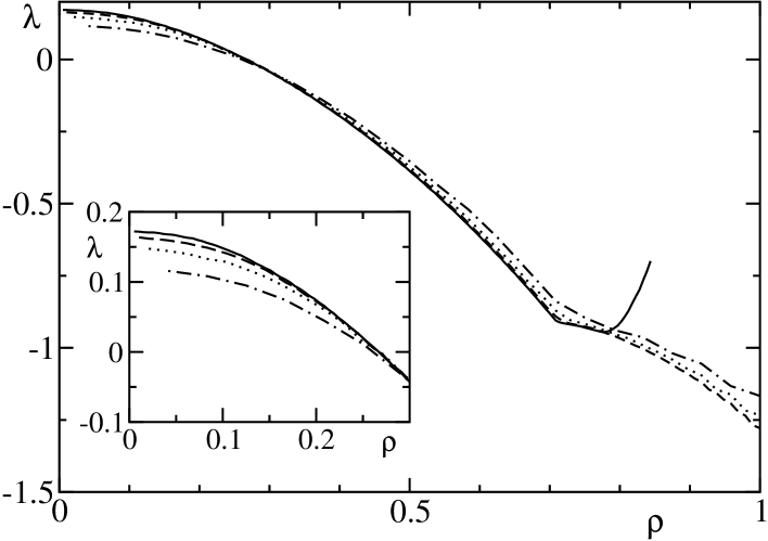
Figure 1: Open-system Lyapunov spectra of Bernoulli maps with $a=1.2$ and $g=1$. Dot-dashed, dotted, dashed and solid curves correspond to $L=24$, 48, 96 and 192, respectively. The last part of the solid curve is truncated because it is numerically unreliable. In the inset, an enlargement of the region around the maximum is reported.

The spectra reported in Fig. 2 correspond instead to different values of $g$ for a fixed length $L$. In the limit $g\rightarrow 0$, the effects of propagation outside the initial window are negligible, so that $\lambda(\rho,g=0)$ reduces to the standard Lyapunov spectrum. In fact, the lowermost curve corresponds to the analytically known expression for the standard Lyapunov spectrum. Upon increasing $g$, the OSLS increases and for $g\to\infty$, we expect it to flatten around the maximum Lyapunov exponent. In the inset of Fig. 2, we have suitably rescaled the $\rho$ axis. The rather good data collapse suggests that the propagation of perturbations does not modify the spectrum structure, but simply leads to an expansion of the $\rho$ scale. Indeed, from the definition of $\rho=l/L$, one can notice that the scale is controlled by the window length $L$.

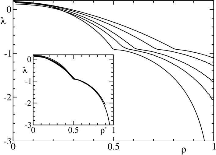
Figure 2: Open-system Lyapunov spectra of Bernoulli maps with $a=1.2$ and $L=96$. From bottom to top, the curves correspond to $g=0$, 1/4, 1/2, 1, and 3/2, respectively. In the inset, the same spectra are plotted after rescaling the $\rho$ axis according to the argument discussed in the text.

However, as anticipated above, in the case of open-system simulations, the space covered by each perturbation increases with time, so that it is reasonable that the label $l$ should be more properly scaled to some effective length $L_{eff}$ rather than to the initial length $L$. Furthermore, it can be conjectured that the effective length increases linearly in time as $L_{eff}=L+2vT$, with some velocity $v$ (the factor 2 is included to account for the growth on both sides of the window). Therefore, the “right” scaled variable should be $\rho^{\prime}=l/[L+2vT]=\rho/(1+2gv)$, and, asymptotically, one expects that $\lambda(\rho,g)$ converges to some $\tilde{\lambda}(\rho^{\prime})$. The good data collapse observed in the inset Fig. 2 points in this direction, although, from the raw data we cannot exclude that the apparent hyperscaling is only an approximation. Indeed, the finite size corrections affecting the various spectra are of the same order as the deviations among the various curves.

In order to study the dependence of the OSLS on $g$ in a more quantitative way, we proceed as follows. Given a spectrum $\lambda(\rho,g)$, we fix a threshold $\lambda_{s}$ and compute the quantity:

$$S(\lambda_{s},g)\doteq\int(\lambda(\rho,g)-\lambda_{s})\,d\rho,$$ (18)

where the integral is restricted to the interval of $\rho$-values where the integrand is positive. For $\lambda_{s}=0$, $S$ reduces to the well known Kolmogorov-Sinai entropy. The dependence of $S$ on $g$ can be observed in Fig. 3 for three different thresholds. The essentially linear behaviour confirms that the increase is due to a propagation process, since the effective length increases linearly with time, i.e., with $g$. If only one propagation velocity $v_{s}$ is present in the evolution, each curve should increase as

$$S(\lambda_{s},g)=S(\lambda_{s},0)(1+2v_{s}g)\quad.$$ (19)

Therefore, the curves obtained for different values of $\lambda_{s}$ should, after rescaling them to the same starting point, overlap. That is, if the velocity $v_{s}$ does not depend on the threshold $\lambda_{s}$, then the plot of $S\,^{\prime}(g)\doteq S(\lambda_{s},g)/S(\lambda_{s},0)$ should be universal. The inset of Fig. 3 reveals however a weak dependence on $\lambda_{s}$: the slopes corresponding to the different thresholds are 0.23, 0.25 and 0.28, indicating that $v_{s}$ ranges in the interval $[0.11-0.14]$. Whether the fluctuations are due to finite size corrections or are an indication of a whole spectrum of velocities, we cannot say. The increase of the velocity when $\lambda_{s}$ decreases suggests, however, that the less unstable directions are characterized by a more efficient propagation.

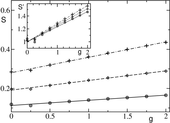
Figure 3: The pseudo entropy $S(\lambda_{s},g)$ defined in Eq. (18) versus $g$ for $\lambda_{s}=-0.7$, $-0.5$ and $-0.3$ (from top to bottom), for Bernoulli maps with $a=1.2$ and $L=96$. In the inset the same data are plotted, with the same symbols, after rescaling, giving the quantity $S\,^{\prime}(g)$ defined in the text.

Bernoulli maps certainly represent the simplest model for testing the spreading properties of perturbations in chaotic systems, but the pecularities of the model (above all, the absence of fluctuations for the local multipliers) may invalidate the generality of the conclusions. Though this is not true for the scaling properties of the standard Lyapunov spectrum, it is nevertheless wise to repeat the analysis above for different models.

For this reason we now discuss the case of asymmetric tent maps, for which

$$f(y)=\begin{cases}{\displaystyle{\frac{y}{b}}}&{\rm if}\quad 0\leq y\leq b\cr\ &\cr{\displaystyle{\frac{1-y}{1-b}}}&{\rm if}\quad b\leq y\leq 1.\end{cases}$$ (20)

While the simulations on this model have been performed for several choices of the coupling $\varepsilon$, and map parameter $b$, the results here presented refer mainly to the $(\varepsilon,b)=(1/3,3/4)$ case. Once more, we observe that the OSLS converges to an asymptotic shape when simulations are performed for increasing time (and thus window size) at a fixed value of $g$. Some OSLS’s are plotted in Fig. 4, where we again see the same flattening tendency for the spectrum and a similar collapse, as observed for the Bernoulli maps. In order to test quantitatively the (visually suggested) hypothetical hyperscaling, we again investigate the behaviour of the pseudo entropy $S(\lambda_{s},g)$ for various choices of the threshold $\lambda_{s}$. The results plotted in Fig. 5 confirm what found before, though indicating a more evident increase in the slopes (in the rescaled representation) of the fits as $\lambda_{s}$ is lowered, thus reinforcing the idea that different velocities are into play. As before, decreasing the threshold $\lambda_{s}$, from $+0.2$ to $0.0$ and to $-0.2$, we observe an increase in the velocity, $v_{S}=0.10,\ 0.12,\ 0.14$, respectively, in agreement with the interpretation, already suggested in the Bernoulli case, of a more efficient propagation of disturbances along more stable directions.

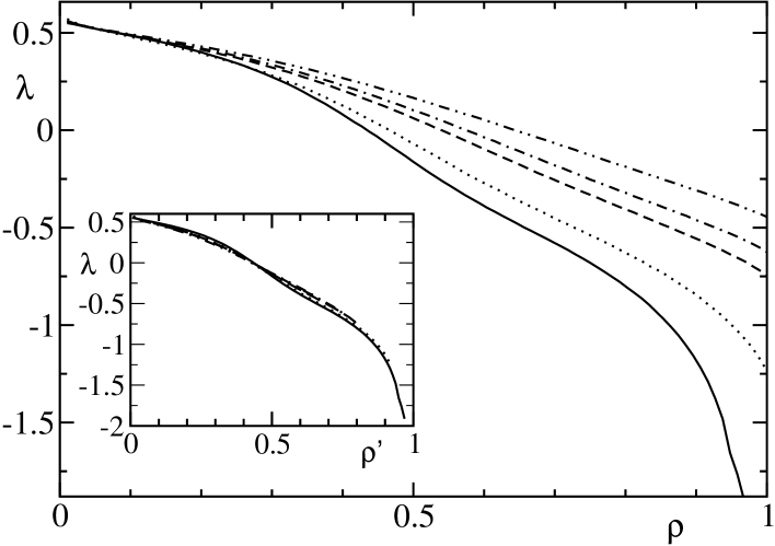
Figure 4: Open-system Lyapunov spectra of asymmetric tent maps, for a window of size $L=96$, with coupling $\varepsilon=1/3$ and $b=3/4$. From bottom to top, the curves correspond to $g=0$, 1/4, 3/4, 1, and 3/2, respectively. In the inset, the same spectra are plotted after suitably rescaling the $\rho$ axis.

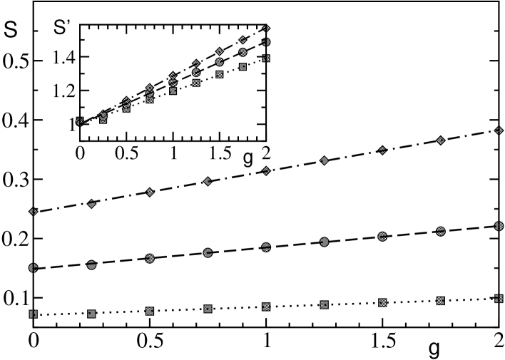
Figure 5: The pseudo entropy $S(\lambda_{s},g)$, defined in Eq. (18), for the same tent maps of the previous figure, versus $g$. From top to bottom, it is $\lambda_{s}=-0.2,\ 0.0\ {\rm and}\ +0.2$. In the inset the ratio $S\,^{\prime}=S(\lambda_{s},g)/S(\lambda_{s},0)$ is plotted, with the same symbols.

Finally, as a prototype of a model with more than one variable per lattice site and also as an example of a system with conservation of volumes, we have studied coupled symplectic maps,

$$p^{i}(t+1)=p^{i}(t)-K\left[\sin{q^{i}(t)}+\varepsilon\left(T^{i+1}(t)-T^{i}(t)\right)\right]$$

$$q^{i}(t+1)=q^{i}(t)+p^{i}(t+1)\ ,$$

where $T^{i}(t)\doteq\sin{[q^{i}(t)-q^{i-1}(t)]}$. Consequently, for the evolution of perturbations, we have,

$$\delta p^{i}(t+1) = \delta p^{i}(t)-K\left[\cos{q^{i}(t)}-\varepsilon(D^{i+1}(t)+D^{i}(t))\right]\delta q^{i}(t)+$$

$$- \varepsilon K\left[D^{i+1}(t)\delta q^{i+1}(t)+D^{i}(t)\delta q^{i-1}(t)\right]$$

and

$$\delta q^{i}(t+1)=\delta q^{i}(t)+\delta p^{i}(t+1)\ ,$$

where $D^{i}(t)\doteq\cos{[q^{i}(t)-q^{i-1}(t)]}$.

Again, different values of the parameters have been chosen, though we present here just the results related to the case $K=5$ and $\varepsilon=1/6$.

In Fig. 6, the OSLS in the case of a window of size $L=96$ (thus, for $2L=192$ Lyapunov exponents) are shown, for several values of $g$. The inset in the same figure points out the good scaling behaviour of these spectra. Performing on them the same analysis as before, through the computation of $S\,^{\prime}$, we find a disturbance propagation velocity $v_{s}=0.050\pm 0.005$ considerably smaller than in the previous cases, though it should be stressed that the coupling strength is now smaller by a factor 2.

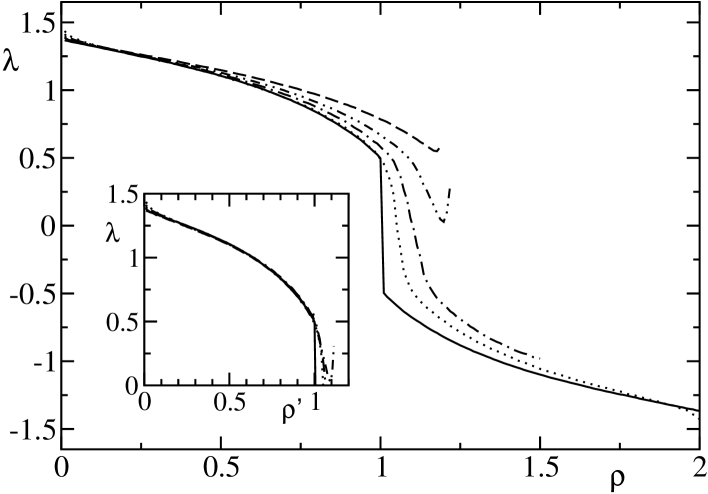
Figure 6: Open-system Lyapunov spectra of coupled symplectic maps for $L=96$ (i.e., $N=192$ exponents). From bottom to top, the curves correspond to $g=0$, 1/4, 3/4, 1, and 3/2, respectively. In the inset, the same spectra are plotted after suitably rescaling the $\rho$ axis.

The velocities obtained through the analysis performed in this section are basically the volume spreading velocities. As mentioned in the beginning of this section, another velocity, $v_{c}$, can be determined from the zero of the spectrum of the convective Lyapunov exponents. In order to compare the two velocities, we have computed also $v_{c}$, using the procedure described in Ref. PTepl94 , to which we refer for more details. Here we limit to report the results of the application of such a method to the models discussed in this paper. In Table I, the two sets of velocities can be mutually compared. For a meaningful comparison with the velocity obtained from the corresponding convective spectra, we have reported there the value of $2v_{s}$, since the effective length implicitly determined when estimating the Lyapunov spectrum over a time $T$, is the average length over such an interval and thus it is half of the final length (if the growth is uniform, as we are assuming). Therefore each velocity has to be doubled, if we want to make a direct comparison with $v_{c}$.

Model	$2v_{s}$	$v_{c}$
Bernoulli $(\varepsilon=1/3)$	$0.24\pm 0.03$	$0.48\pm 0.01$
Tent $(\varepsilon=1/3)$	$0.24\pm 0.04$	$0.90\pm 0.01$
Tent $(\varepsilon=1/6)$	$\ 0.09\pm 0.02$	$0.64\pm 0.01$
Symplectic $(\varepsilon=1/6)\ \$	$0.09\pm 0.01$	$0.83\pm 0.01$

Table 1: Synoptic table containing the velocities determined from the open-system Lyapunov spectra and from the zero of the convective Lyapunov spectra for the classes of maps discussed in the text.

We see that in all the cases, the volume spreading velocity is significantly different from (and smaller than) the propagation velocity of perturbations, thus indicating that at least two mechanisms exist in spatio-temporal chaos that contribute to the propagation of information. Indeed, a moment’s reflection reveals a crucial difference between the two velocities. On the one hand, we see that if the local multipliers change all by the same constant factor, $r$, the resulting convective Lyapunov spectrum is shifted by $\ln r$ and, as a consequence, the velocity $v_{c}$, corresponding to the crossing point with the $v$-axis, changes. On the other hand, the velocity $v_{s}$ remains unchanged. In fact, we believe it is not by chance that $v_{s}$ turns out to be approximately the same for the same values of the coupling strength (see the table): it measures how the spatial coupling forces an ensemble of perturbations to cover all neighbouring directions. Thus, in principle, it can be defined even for a stable system. In a sentence, we could summarize stating that $v_{c}$ reflects the (chaotic) features of the local dynamics, whereas $v_{s}$ exploits the efficiency of the of the coupling in favouring the propagation of information.

V Scaling behaviour of the invariant measure and concluding remarks

In this last section we exploit the knowledge of the scaling behaviour of the OSLS to shed light on the corrections to the Kaplan-Yorke formula arising from the spatial coupling. We start neglecting the integration over the external degrees of freedom (see Eq. (12)). In this approximation, we are entitled to use equations (9) and (10), with the warning that now the Lyapunov exponents do depend on time. Under the assumption that hyperscaling holds, Eq. (11) still applies, with the length $L$ replaced by its effective value over a time $T$,

$$\tilde{D}_{KY}(T,L)=d(1+2vg)L=dL+2dvT$$ (21)

In order to independently check the linear dependence of $\tilde{D}_{KY}$ on $g$, we have studied the behaviour of $d_{KY}=\tilde{D}_{KY}(T,L)/L$, by integrating the spectra obtained for different values of $g$, in the case of coupled Bernoulli maps. From the above argument, we expect that $d_{KY}=d(1+2v_{KY}g)$, where $v_{KY}$ is, in principle, still another velocity of propagation, though much of the same nature as $v_{s}$.

The data plotted in Fig. 7 indicate indeed a quite clean linear growth. The deviation of the value corresponding to $g=1/4$ is certainly due to finite-size corrections, since it has been obtained for the shortest time compared to the other points, while the datum corresponding to $g=0$ ($d_{KY}(0)=0.39$) is obtained from the standard Lyapunov spectrum (see Ref. IPRT90 ), and is therefore not affected by numerical convergence problems. From the figure, the slope of the curve $d_{KY}(g)$ is 0.09 and from this (and from $d_{KY}(0)$) it follows that $v_{KY}=0.12$, well consistent with the value, $v_{s}$, obtained from the generalized KS-entropy approach.

We can now use Eq. (9) to transform the dependence of $\tilde{D}_{KY}$ on time $T$ into a dependence of $D_{KY}$ on the resolution $\varepsilon$. Indeed, inverting Eq. (9), we have

$$T=\frac{\ln\varepsilon}{\lambda_{d}}\quad,$$ (22)

where $\lambda_{d}\doteq\lambda(\rho=d)$.

Inserting then Eq. (22) in Eq. (21), we obtain

$$D_{KY}(\varepsilon,L)=dL+\frac{2vd}{\lambda_{d}}\ln\varepsilon$$ (23)

which again reveals a logarithmic dependence on the resolution. At variance with the past derivations of similar formulas, however, the multiplicative factor in front of the logarithmic correction follows now from a well documented discussion of the dynamical evolution.

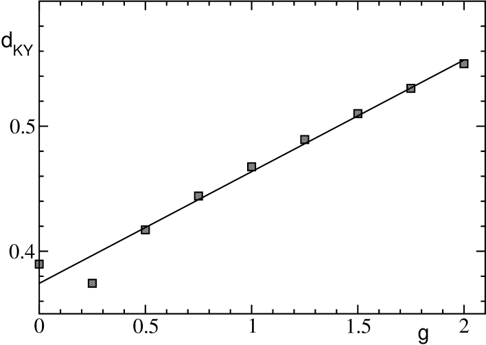
Figure 7: The scaled dimension $d_{KY}$ versus $g$, as computed from the Kaplan-Yorke formula, for the Bernoulli coupled map lattice.

However, we should not forget that the above formula represents a lower bound on the dimension, $D_{KY}$, since we have neglected the integral over ${\bf x}_{\perp}^{0}$ in Eq. (12) that accounts for the uncertainty on the inner variables induced by the initial lack of knowledge on the outer degrees of freedom. An accurate quantification of the corresponding propagation of information is far from trivial, since it may be controlled by nonlinear mechanisms as it is known to happen in some situations. A typical case, where this is certainly true is that of the so-called stable chaos CLP98 , i.e. of the irregular behaviour emerging even in the presence of a negative Lyapunov spectrum. In that case, no extensive contribution to $D$ exists since $d=0$ and the previously discussed logarithmic correction is absent too. Nevertheless, finite-amplitude perturbations may enter the window of interest carrying relevant information.

In order to complement the lower bound above, we present here a heuristic argument that allows us determining also an upper bound, through an estimate of the effect of the disturbances propagating from the boundaries into the region of observation. It should be clearly stated that the validity of the following argument relies on the assumption that nonlinear mechanisms are negligible.

From the convective Lyapunov exponents, we know that a perturbation originating at the boundary at time 0, is amplified by a factor $\exp{\Lambda_{c}(\ell/T)T}$, after a time $T$ at a distance $\ell$. Let us assume that, according to Eq. (22), the time $T$ corresponds to a resolution $\ln\varepsilon/\lambda_{d}$. Then, the maximum distance travelled by the external perturbation while still being larger than $\varepsilon$ can be implicitly determined by the equation

$$\lambda_{d}=\Lambda_{c}(\ell/T)=\Lambda_{c}\left(\frac{\ell\lambda_{d}}{\ln\varepsilon}\right)\ .$$ (24)

Let us now $v^{\prime}$ denote the velocity such that $\Lambda_{c}(v^{\prime})=\lambda_{d}$ (if the whole convective spectrum is larger than $\lambda_{d}$, $v^{\prime}$ must be assumed equal to the maximal possible velocity, which, in the case of nearest neighbour coupling, is just equal to 1). Eq. (24) implies that

$$\ell=\frac{v^{\prime}}{\lambda_{d}}\ln\varepsilon\quad.$$ (25)

By assuming that the distribution of the state variable is independent in all the $\ell$ sites, one finds that $f\ell$ (where $f$ denotes the number of variables per lattice site), represents an upper bound to the correction due to the external degrees of freedom. Accordingly, this correction has again the same structure as the previous one; altogether, one finds that

$$D_{c}(\varepsilon,L)\leq dL+\frac{2(dv+fv^{\prime})}{\lambda_{d}}\ln\varepsilon.$$ (26)

Thus, we see that the dependence of the effective dimension on $\varepsilon$ remains weaker than the $1/\varepsilon$ behaviour deduced indirectly from the treatment in Ref. CE99 . We interpret this as the indication that the rigorous bound determined in Ref. CE99 can be improved. Neverthless, a more detailed understanding of the propagation of perturbations is also required, in order to shed further light on the exact structure of the logarithmic corrections. We are currently exploring the possibility to directly quantify the amplitude of volume-perturbations in a simplified class of systems where most of the calculations can be carried on analytically CP03 .

The above analysis has been perforemd under the implicit assumption that $|\ln\varepsilon|<\alpha L$ (where $\alpha$ is a suitable dimensional factor). This limitation is equivalent to the one encountered in the paper by Collet & Eckmann CE99 , where it is stated that the bound (6) applies only in the region where $\varepsilon>a/L$. The reasons for these limitations are due to nonlinear effects. In the previous section we have seen that in the linear approximation any perturbation, initially restricted to $W_{L}$, sooner or later diverges along all the $L$ existing directions (inside the window). However, nonlinear corrections may become important much before the amplitude of the perturbation becomes of order 1 inside $W_{L}$. Indeed, we have seen that perturbations grow outside $W_{L}$, too; in particular, those that initially decay inside $W_{L}$, grow outside the window. As soon as their amplitude becomes ${\mathcal{O}}(1)$ in the outer part, the effect of nonlinearities cannot be any longer neglected even inside $W_{L}$, though their amplitude is therein very small. Since we have seen that high resolutions correspond to relatively long time, we cannot expect our approach to hold for those tiny scales where $|\ln\varepsilon|/L$ is no longer small.

It is now worth commenting about the relationship between the open-system Lyapunov exponents introduced in this paper and the previously devised chronotopic Lyapunov approach LPT96 ; LPT97 . There, it was conjectured that all linear stability properties of 1d spatially extended dynamical system can be obtained from the entropy potential: a function of the spatial and temporal growth rate of generic perturbations. Although we have not been able to find the specific link with the OSLS, there is no reason to think that the information contained in that class of Lyapunov spectra is not contained in the entropy potential. Finding the relationship between the two approaches would be very interesting not only from a conceptual point of view, but also because it would allow for a much easier computation of the OSLS. We must, indeed, recall that an accurate determination of Lyapunov spectra in open systems is hindered by the high accuracy that it requires: this limitation is certainly crucial in the context of continuous space-time systems such as, e.g., the complex Ginzburg-Landau and the Kuramoto-Sivahsinsky equations.

Finally, we expect the open system approach to be of some relevance also in connection with the nonequilibrium dynamics of Hamiltonian systems. For instance, in Ref. G02 , Gallavotti was interested in the expansion rate of local (in space) volumes. This is nothing but the function $S$, defined by Eq. (18), for $\lambda_{s}$ corresponding to the minimum Lyapunov exponent.

References

- (1) H. Kantz and T. Schreiber, Time-series analysis, Cambridge University Press 1999.
- (2) Y. Pomeau, Compt. Rend. Acad. Sci. Paris, t. 300, Série II 7 235 (1985).
- (3) P. Grassberger, Physica Scripta 40 346 (1989).
- (4) P. Collet, J.-P. Eckmann, Commun. Math. Phys. 200 699 (1999).
- (5) L.S. Tsimring, Phys. Rev. E 48 3421 (1993).
- (6) L.N. Korzinov and M.I. Rabinovich in Applied Nonlinear Dynamics (Saratov University Press, 1994), Vol. 2, 59-69.
- (7) A.N. Kolmogorov, and V.M. Tikhomirov, Selected Works of A.N. Kolmogorov Vol. III, A.N. Shirayayev ed. Dordrecht, Kluwer 1993.
- (8) A. Torcini, A. Politi, G.P. Puccioni, G. D’Alessandro, Physica D 53 85 (1991).
- (9) A. Politi and G.P. Puccioni, Physica D 58 384 (1992).
- (10) E. Olbrich, R. Hegger, and H. Kantz, Phys. Lett. A 244 538 (1998).
- (11) A. Politi and A. Witt Phys. Rev. Lett. 82 3034 (1999).
- (12) J.-P. Eckmann and D. Ruelle, Rev. Mod. Phys. 57, 617 (1985).
- (13) R.J. Deissler and K. Kaneko, Phys. Lett. A 119 397 (1987) .
- (14) A.Politi and A.Torcini, Europhys.Lett. 28 545 (1994).
- (15) S. Isola, A. Politi, S. Ruffo, and A. Torcini, Phys. Lett. A 143, 365 (1990).
- (16) F. Cecconi, R. Livi, and A. Politi, Phys. Rev. E 57, 2703, (1998).
- (17) P. Cipriani and A. Politi, in preparation.
- (18) S. Lepri, A. Politi, A. Torcini, J. Stat. Phys. 82, 1429 (1996).
- (19) S. Lepri, A. Politi, A. Torcini, J. Stat. Phys. 88, 31 (1997).
- (20) G. Gallavotti, Large deviations, fluctuation theorem and Onsager-Machlup theory in nonequilibrium statistical mechanics., preprint FM 2002-03, available on http://ipparco.roma1.infn.it.