Frequency spanning homoclinic families.

Abstract.

A family of maps or flows depending on a parameter $\nu$ which varies in an interval, spans a certain property if along the interval this property depends continuously on the parameter and achieves some asymptotic values along it. We consider families of periodically forced Hamiltonian systems for which the appropriately scaled frequency $\overline{\omega}(\nu)$ is spanned, namely it covers the semi-infinite line $[0,\infty).$ Under some natural assumptions on the family of flows and its adiabatic limit, we construct a convenient labelling scheme for the primary homoclinic orbits which may undergo a countable number of bifurcations along this interval. Using this scheme we prove that a properly defined flux function is $C^{1}$ in $\nu.$ Combining this proof with previous results of RK and Poje, immediately establishes that the flux function and the size of the chaotic zone depend on the frequency in a non-monotone fashion for a large class of families of Hamiltonian flows.

1. Introduction

The modern approach to the study of a dynamical system identifies solving the problem with finding the global structure of phase space. On the other hand, bifurcation theory has mostly concentrated on local behavior in the parameter space (so even when global phase space bifurcations are considered, they are always considered in a small neighborhood of a given parameter value). Here we suggest that global analysis with respect to parameters leads to understanding of the phase space structure in parameter regimes which are unreachable by the currently known analysis techniques. In particular, we examine some features of the global dependence of periodically forced systems with finite forcing amplitude on the forcing frequency.

The study of the effect of periodic forcing on homoclinic loops has been thoroughly investigated since the times of Poincaré. Analytical understanding of such systems has been attained in three possible limits (see [1],[6]): the fast and slow oscillations limits and the small forcing limit (see figure 1). For fast oscillations averaging methods apply, and together with KAM theory, these are used to obtain upper bounds on the separatrix splitting. These bounds are exponentially small in the frequency ([17],[14]). Lower bounds on the separatrix splitting involve delicate analysis which has been proved, under some structural assumptions on the flow, only in recent years (see [5] and references therein). The slow oscillations regime corresponds to the region where adiabatic theory applies. Two approaches have been applied to this limit - the first one corresponds to extending classical adiabatic theory to separatrix crossing ([15],[21]) and the other corresponds to examining the geometrical properties of stable and unstable manifolds to hyperbolic manifolds with slowly varying motion on them (see [9],[10],[20],[4]). Most of the analytical studies have been performed in the small oscillations regime in which perturbation methods apply (see ([6]) and references therein). The most important ingredient from these studies to the current paper is the existence of a flux mechanism via lobes (see [2],[11],[12],[19],[18]).

Here we show that for a large class of systems, the phase space structure and its associated transport properties have some common non-monotone dependence on the frequency of the forcing term. Namely, we establish that in some cases, even for finite size oscillations, there exists a function which depends on the frequency continuously. After some natural scaling, this function is simply the sum of the areas of the incoming lobes per period, normalized by the forcing period. Hence, results obtained in the fast and slow limits supply information regarding the behavior in the intermediate regime where no analytical methods apply (see figure 1). Furthermore, this proposed viewpoint leads to a non-traditional scaling of the flow which is relevant for studying its behavior near homoclinic tangles. This paper supplies mathematical formulation and generalization of the common work of the author with A. Poje [18], in which similar issues were considered in the context of fluid mixing.

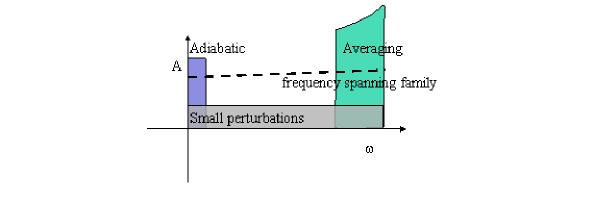
Figure 1. Frequency spanning families.

The paper is organized as follows: In the first section we define the class of forced Hamiltonian families which we consider. Roughly, these are forced Hamiltonian families with split separatrices, for which the splitting exists for all positive parameter values and as the family parameter varies the scaled frequency includes the semi-infinite line. In the second section we construct a labelling scheme for primary homoclinic orbits, which relies on the concepts of unstable ordering introduced by Easton [3]. This labelling scheme is valid for all parameter values and behaves well across homoclinic bifurcations. In the third section we prove the main result of this paper - that the flux through the homoclinic loop depends continuously (in fact it is $C^{1}$) in the spanning parameter of the family (in [18] we considered a restricted class of systems for which the continuity of the flux followed immediately). To prove this result several properties of the lobes are studied, the details are included in appendix 2. In the fourth section we recall the proof of RK and Poje, showing that the flux is non-monotone in the scaled frequency and recall the implications of these results, especially in view of their implications regarding the stochastic zone width (see [22]). Section five includes a demonstration of these concepts for the forced center-saddle bifurcation problem. Conclusions are followed by two appendices - in the first the homoclinic scaling is discussed whereas in the second detailed proofs of some properties of the lobes are included, the relation between the flux and the areas of the exit and entry sets is explained, and the adiabatic limit is discussed.

2. Frequency-spanning families.

Consider a one-and-a-half degree of freedom Hamiltonian $H(x,y,\omega(\nu)t+\theta;\nu)$ which is $2\pi$ periodic in its last argument and depends smoothly on the parameter $\nu\in[0,\nu^{\ast}),$ where $\nu^{\ast}>0$ may be finite or infinite. This Hamiltonian may be written in the form

(2.1) $$H(x,y,\omega(\nu)t+\theta;\nu)=H_{0}(x,y;\nu)+H_{1}(x,y,\omega(\nu)t+\theta;\nu)$$

where the second term has zero time average:

$$\int_{0}^{\frac{2\pi}{\omega}}H_{1}(x,y,\omega(\nu)t+\theta;\nu)dt\equiv 0$$

and may be as large as the first one. Assume the Hamiltonian system of (2.1):

(2.2) $$\frac{dx}{dt} =\frac{\partial H(x,y,\omega(\nu)t+\theta)}{\partial y}=u_{0}(x,y;\nu)+u_{1}(x,y,\omega(\nu)t+\theta;\nu)$$

$$\frac{dy}{dt} =-\frac{\partial H(x,y,\omega(\nu)t+\theta)}{\partial x}=v_{0}(x,y;\nu)+v_{1}(x,y,\omega(\nu)t+\theta;\nu)$$

satisfies the following structural assumptions:

A1:

$H_{0}$ and $H_{1}$ are $C^{r},r>2$ functions of all their arguments, $H_{1}$ is $2\pi$ periodic with zero mean in its last argument .

A2:

For all $\nu$ values in $[0,\nu^{\ast}]$, (2.2) possesses a hyperbolic periodic orbit which depends smoothly on $\nu$.

A3:

The family of Hamiltonians spans the frequency parameter: the frequency $\omega(\nu)$ is a smooth $C^{r},r>2$ function, and it maps the interval $[0,\nu^{\ast})$ onto the semi-infinite line: $[0,\infty)=\{\omega(\nu)|\nu\in[0,\nu^{\ast})\}.$ Furthermore, $\omega(\nu)\rightarrow 0$ only at one of the interval’s boundaries and at no interior point.

A4:

For $\omega=0$, for any phase $\theta$, at least one branch of the stable and unstable manifolds of that periodic orbit coincide to form a homoclinic loop. Furthermore, the manifolds and the homoclinic loops created at $\omega=0$ depend smoothly on $\theta$, and the phase space area enclosed by these homoclinic loops, $\ \mu(R^{L,R}(\theta))$, is non-constant and has a finite number of extrema:

$$\frac{d}{d\theta}\mu(R^{L,R}(\theta))\neq 0\text{, for all }\theta\in[0,2\pi]\backslash\{\theta_{1},\theta_{2},...,\theta_{N_{0}}\}\text{.}$$

For concreteness, with no loss of generality, we assume that at $\omega=0$ the manifolds topology is of a lying figure eight (closed geometry) or of a fish swimming to the left (open geometry), so the left branches always coincide at $\omega=0$, see figure 2.

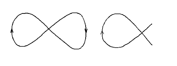
Figure 2. Manifolds geometry at $\omega=0$.
a. Closed geometry (lying 8) b. Open geometry (fish).

For $\omega\neq 0$, consider the standard global Poincaré map $F_{0}$ of the extended phase space $(x,y,t),$ which is simply the time-$\frac{2\pi}{\omega}$ map of the time dependent flow (here $\theta$ is introduced to account for phase variations):

$$F_{\theta}:(x(0;\theta,\nu),y(0;\theta,\nu))\rightarrow(x(\frac{2\pi}{\omega};\theta,\nu),y(\frac{2\pi}{\omega};\theta,\nu))$$

The two dimensional symplectic map $F_{0}$ has, by the above assumptions, a hyperbolic fixed point $\gamma(\nu)$ with its associated stable and unstable manifolds. $p$ is a primary homoclinic point of $\gamma(\nu)$ iff the open segments of the unstable (respectively stable) manifold connecting $\gamma(\nu)$ with the homoclinic point $p$, $U(\gamma(\nu),p)$ (respectively $S(\gamma(\nu),p)$) do not intersect ([3],[19]):

$$U(\gamma(\nu),p)\cap S(\gamma(\nu),p)=\emptyset.$$

The points $p_{i}^{k}$ in figure 3 are all primary homoclinic points, whereas the intersection points of the manifolds inside the shaded region in figure 6 are homoclinic points which are not primary. We assume:

A5:

For all $\nu\neq 0$ there is a finite number of primary homoclinic orbits. Furthermore, for each intersecting branches of the manifolds there exist at least two primary homoclinic orbits which are topologically transverse.

A6:

The number of primary homoclinic bifurcations is bounded in any bounded open interval of $\nu$ for all $\nu\neq 0$. The order of the primary homoclinic bifurcations is uniformly bounded by the integer $M.$

For convenience of notation, let us assume that $M<10.$

Finally, to establish asymptotic behavior in the frequency, we assume there exists an appropriate scaling so that the scaled separatrix length scales and the maximal velocity along the separatrix are of order one:

A7:

There exist smooth ($C^{r}$ in $\nu$) non-vanishing scaling functions, $W_{0}(\nu),W_{1}(\nu),$ $L_{x}(\nu),L_{y}(\nu),L_{\max}(\nu),$ such that in the scaled variables:

(2.3) $$(\overline{x},\overline{y}) =\left(\frac{x}{L_{x}(\nu)},\frac{y}{L_{y}(\nu)}\right),\ \ \ \ \overline{t}=\frac{W_{0}(\nu)}{L_{\max}(\nu)}t,\ \$$

(2.4) $$\ \ \ \overline{H} =\frac{L_{\max}(\nu)}{W_{0}(\nu)L_{x}(\nu)L_{y}(\nu)}H,$$

(2.5) $$(\overline{u}_{i,}\overline{v}_{i}) =\frac{L_{\max}(\nu)}{W_{i}(\nu)}\left(\frac{u_{i}}{L_{x}(\nu)},\frac{v_{i}}{L_{y}(\nu)}\right),\text{ \ }i=1,2$$

the scaled system:

(2.6) $$\frac{d\overline{x}}{d\overline{t}} =\overline{u}_{0}(\overline{x},\overline{y};\nu)+A\overline{u}_{1}(\overline{x},\overline{y},\overline{\omega}\overline{t}+\theta;\nu)$$

$$\frac{d\overline{y}}{d\overline{t}} =\overline{v}_{0}(\overline{x},\overline{y};\nu)+A\overline{v}_{1}(\overline{x},\overline{y},\overline{\omega}\overline{t}+\theta;\nu)$$

with the two non-dimensional parameters $A,\overline{\omega}$ :

$$A(\nu)=\frac{W_{1}(\nu)}{W_{0}(\nu)},\ \ \overline{\omega}(\nu)=\omega(\nu)\ \frac{L_{\max}(\nu)}{W_{0}(\nu)}\ \ .$$

satisfies assumptions A1-A6. Furthermore, for the scaled system, the width and length of the separatrix and the maximal velocity along it are all of order one for all $\nu\in(0,\nu^{\ast})$.

$A(\nu)$ measures the relative strength of the temporal oscillations to the mean flow whereas $\overline{\omega}(\nu)$ compares the oscillation’s time scale with the travel time along the separatrix loop (outside of the saddle orbit neighborhood). We assert that the magnitude of these two parameters supplies complete information on the qualitative behavior of the system (2.6) and hence on the original system. Notice that assumption A3 is now made with respect to the scaled frequency.

Definition 1.

A family of Hamiltonian systems depending on a parameter $\nu$ which satisfies assumptions A1-A7 is called a frequency-spanning homoclinic family, and $\nu$ is called a frequency-spanning parameter.

A few remarks are now in order:

• Assumptions A1-A7 clearly hold in the standard near integrable case (small $A(\nu)$) where the steady flow has a homoclinic loop of fixed size (independent of $\nu$), the perturbation is generic (so A5 and A6 are satisfied), and its frequency, $\omega(\nu)=\nu,$ spans the half real line.

• A5 refers only to primary homoclinic bifurcations - otherwise it would have been violated generically, see [23] and references therein.

• In the near-integrable case the scaling functions may be simply extracted from the integrable flow, see for example section 6. In appendix 1, after some notation is established in the next section, we propose an algorithm for defining the characteristic scales in the finite amplitude size forcing case.

• The assumptions here are slightly weaker than the ones in [18]: in particular A5 and A6 replace the stronger assumption of [18] that there exists one topologically transverse primary homoclinic orbit which depends continuously on $\nu$, a property which may be easily violated in applications. Relaxing this assumption requires the introduction of a new labelling scheme for the homoclinic points which takes into account the possible annihilation of primary homoclinic points.

Hereafter we assume the forced system is in its scaled form and we drop all the over bars when non-ambiguous, as described next.

3. labelling scheme for the primary homoclinic points

Denote by $P(\nu)=$ $\{p^{r_{n}(\nu)}(\nu),n=1,...,N(\nu)\}$ the topologically transverse primary homoclinic orbits of $\gamma(\nu)$ belonging to the left branch (for simplicity of notation we consider hereafter only the left branch of the loop), where $p^{r_{n}(\nu)}(\nu)=\{p_{i}^{r_{n}(\nu)}(\nu)\}_{i=-\infty}^{\infty}=\{F^{i}p_{0}^{r_{n}(\nu)}(\nu)\}_{i=-\infty}^{\infty}$, namely the discrete index $i$ denotes iterations under the map and the index $r_{n}(\nu)$ denotes the label of the specific orbit. Each such transverse homoclinic point, $p_{i}^{r_{n}}(\nu),$ defines a region, $R_{i}^{r_{n}}(\nu),$ enclosed by the closed segments of the stable and unstable manifolds which emanate from the fixed point and meet at $p_{i}^{r_{n}}(\nu),$ namely

(3.1) $$\partial R_{i}^{r_{n}}(\nu)=U[\gamma(\nu),p_{i}^{r_{n}}(\nu)]\cup S[\gamma(\nu),p_{i}^{r_{n}}(\nu)],$$

where, clearly

$$R_{i}^{r_{n}}(\nu)=F^{i}R_{0}^{r_{n}}(\nu).$$

Denote by $0<\nu_{1}<\nu_{2}<....$ the ordered parameter values at which primary homoclinic bifurcations occur (by A6 this may be done), and by $\Upsilon$ the set of all primary homoclinic bifurcation values in $[0,\nu^{\ast})$: $\Upsilon=\{$ $\nu_{1},\nu_{2},...\}$. In figures 3 and 4  we illustrate a possible behavior of the manifolds before and after a primary homoclinic bifurcation occurs. We say that $p^{r_{n}(\nu)}$ undergoes a homoclinic bifurcation at $\nu_{i}$ if $p^{r_{n}(\nu_{1})}$ is a tangent homoclinic orbit. Next we construct a labelling of the orbits in $P(\nu)$ which is convenient even across homoclinic bifurcations.

Lemma 1.

Consider a frequency spanning homoclinic family. Then, there exists a labelling scheme for the primary homoclinic orbits satisfying the following properties:

1. $r(\nu)$ is piecewise constant, changing only at values of $\nu$ at which $p^{r(\nu)}(\nu)$ undergoes a homoclinic bifurcation.

2. The labelling scheme respects the unstable ordering, so that $r_{n}(\nu)<r_{m}(\nu)$ iff $p_{0}^{r_{n}(\nu)}(\nu)<_{u}p_{0}^{r_{m}(\nu)}(\nu)$, namely (see [3]):

   (3.2) $$U[\gamma(\nu),p_{0}^{r_{n}}(\nu)]\subset U[\gamma(\nu),p_{0}^{r_{m}}(\nu)]\text{ \ \ for \ \ }r_{n}<r_{m}.$$

Proof.

By construction. We construct such a labelling scheme inductively, in the intervals $(\nu_{k},\nu_{k+1}),$ starting with the interval $(\nu_{0}=0,\nu_{1}).$

By A5, $N(\nu)\geq 2$ for all $\nu\neq 0$. Since the Poincaré. map is orientation preserving and since only topologically transverse intersections are counted, $N(\nu)$ is even. By assumption A6, there exists a well defined limit of the number of primary homoclinic orbits as $\nu\rightarrow 0^{+}$, so that $N(0^{+})$ is well defined and is finite, and $\nu_{1}>0$. For $0<\nu<\nu_{1}$, let $r_{n}(\nu)=n,n=1,...,N(0^{+}).$ The labelling is chosen to obey the unstable ordering $p_{0}^{i}(\nu)<_{u}p_{0}^{j}(\nu)$ for $i<j,$ where we identify:

(3.3) $$p_{0}^{r_{N(\nu)+1}}(\nu)\equiv p_{1}^{r_{1}}(\nu)=Fp_{0}^{r_{1}}(\nu),\text{ and }p_{0}^{r_{0}}(\nu)\equiv p_{-1}^{r_{N(\nu)}}(\nu)=F^{-1}p_{0}^{r_{N(\nu)}}(\nu).$$

These rules determine the labelling for $0<\nu<\nu_{1}$ up to a cyclic permutation, and do not define the origin (which homoclinic point is $p_{0}^{1}(\nu)$). To remove the first ambiguity, define the labelling so that as $\nu\rightarrow 0^{+}$, the first homoclinic orbit defines the region of maximal area: $\mu(R_{0}^{1}(0^{+}))=\max_{n}(\mu(R_{0}^{n}(0^{+}))$. To remove the second ambiguity, we define the origin ($i=0)$ as the point for which the boundaries of  $R_{i}^{1}(0^{+})$ are of minimal length; Denote the arc length of the boundary of $R_{i}^{r_{n}}(\nu)$ by $|\partial R_{i}^{r_{n}}(\nu)|$. Notice that $|\partial R_{i}^{r_{n}}(\nu)|\rightarrow\infty$ as $i\rightarrow\pm\infty$. Let $p_{0}^{1}(\nu)$, satisfy $|\partial R_{0}^{1}(\nu)|=\min_{i}|\partial R_{i}^{1}(\nu)|$. When there are no degeneracies (here, when the maximal area is achieved at a unique orbit and the minimal boundary length is achieved at a unique homoclinic point) this procedure determines uniquely the labelling of the topologically transverse homoclinic orbits for $0<\nu<\nu_{1}.$ If a degeneracy occurs, choose any one of the finite number of the maximizing (respectively minimizing) orbits (respectively points).

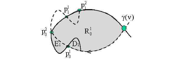
Figure 3. Primary homoclinic points.
Here $N(\nu)=2,\nu<\nu_{1}$ of figure 5.

Given the labelling $Lbl(\nu_{k-1}^{+})=\{r_{1},r_{2},...,r_{N(\nu)}\}$, for $k\geq 1$, so that $Lbl(\nu_{k-1}^{+})=Lbl(\nu)$ for $\nu\in(\nu_{k-1},\nu_{k})$, we construct $Lbl(\nu_{k}^{+})$ as follows:

Case 1.

If the associated homoclinic orbit, $p_{i}^{r_{n}}(\nu)$, depends continuously on $\nu$ at $\nu_{k}$ leave $r_{n}$ unchanged.

Case 2.

If $p_{i}^{r_{n}}(\nu)$ cease to exist for $\nu>\nu_{k}$ , delete $r_{n}$ from $Lbl(\nu_{k}^{+}).$

Case 3.

If $M$ additional homoclinic orbits are created between (along the unstable ordering) $p_{i}^{r_{n}}(\nu)$ and $p_{i}^{r_{n+1}}(\nu),$ insert the $M$ labels, $r^{j}=r_{n}+j\cdot 10^{-k}$, $j=1,...,M$, so that $Lbl(\nu_{k}^{+})=\{r_{1},r_{2},..,r_{n},r_{n}+10^{-k},r_{n}+2\cdot 10^{-k},...,r_{n}+M\cdot 10^{-k},r_{n+1},...,r_{N(\nu)}\}$

By construction the labelling scheme respects the unstable ordering and does not change labels unless homoclinic bifurcation occur, as claimed. Notice that the first case in the proof includes two possibility which are topologically equivalent - the first is that the homoclinic orbit $p_{i}^{r_{n}}(\nu_{k})$ is not involved in the homoclinic bifurcation and the second possibility is that $p_{i}^{r_{n}}(\nu_{k})$ is a tangent periodic orbit with odd order tangency so that no topological bifurcation occurs at $\nu_{k}$. ∎

For any $\nu$ we have constructed a finite, ordered set of labels $Lbl(\nu)=\{r_{1},r_{2},...,r_{N(\nu)}\}$ (so $r_{1}<r_{2}<..<r_{N(\nu)}$) with corresponding homoclinic orbits which satisfy (3.2). The ordering $k(r(\nu)),r\in Lbl(\nu)$ enumerates the primary homoclinic orbits in $P(\nu)$ by their unstable ordering. While the $r^{\prime}s$ depend smoothly on $\nu$ as long as $p_{i}^{r}(\nu)$ has not bifurcated, $k(r(\nu))$ can be discontinuous in $r(\nu)$ due to bifurcations of orbits $p_{i}^{r^{\prime}}(\nu)$ with some $r^{\prime}<r$.

For example, in the simplest, generic case of quadratic tangency, if at $\nu_{1}$ two primary homoclinic orbits are created between (in the sense of the unstable ordering) the $j$th and the $j+1$ homoclinic orbits which existed for $\nu<\nu_{1}$, then these will be labeled as $r=j.1,r^{\prime}=j.2,$ so that $p_{0}^{j}$ $<_{u}p_{0}^{j.1}<_{u}p_{0}^{j.2}<_{u}p_{0}^{j+1}(\nu),$ as demonstrated in figure 4:

(3.4) $$P(\nu)|_{\nu_{1}<\nu<\nu_{2}}=\{p^{1}(\nu),p^{2}(\nu),...,p^{j}(\nu),p^{j.1}(\nu),p^{j.2}(\nu),p^{j+1}(\nu),...,p^{N(0^{+})}(\nu)\}.$$

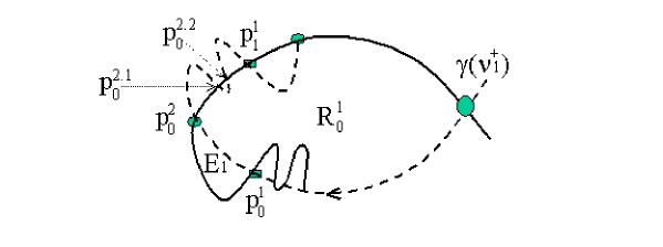
Figure 4. labelling after the first bifurcation.
$\nu=$$\nu$ where $\nu_{1}<$$\nu$$<\nu_{2}$ see figure 5.

By construction, for $0<\nu<\nu_{1}$, $r_{k}=k,$ or equivalently, $k(r;\nu)=r$. On the other hand, for $\nu_{1}<\nu<\nu_{2}$, for the generic case of (3.4) we have $Lbl(\nu)|_{\nu_{1}<\nu<\nu_{2}}=\{1,2,..,j,j.1,j.2,j+1,...,N(0^{+})\}=\{r_{1},..,r_{N(0^{+})+2}\}$ so

$$k(r;\nu)=\left\{\begin{array}[c]{l}r\text{ \ \ \ \ \ \ \ \ \ for }r\leq j\\ [r]+[(r-[r])\cdot 10]\text{ \ \ for }j<r<j+1\\ r+2\text{ \ \ for }r\geq j+1,\end{array}\right.\text{ \ \ \ \ for \ }\nu_{1}<\nu<\nu_{2}$$

and we see that $k(r;\nu)$ changes at $\nu_{1}$ for all $k>j,$ hence, as opposed to the $r_{n}$’s, it does not serve as a good labelling system for the homoclinic orbits across bifurcations.

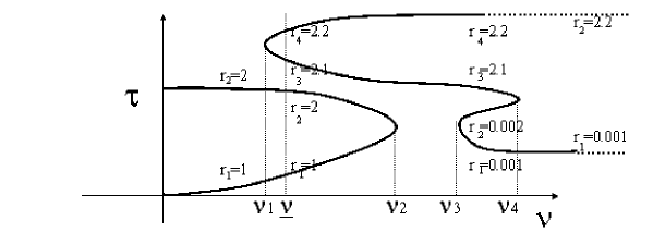
Figure 5. Primary homoclinic bifurcation diagram (schematic).
$\tau$ represents natural parametarization along the unstable manifold.

4. Lobes topology

Consider now a fixed $\nu$ value, with $Lbl(\nu)=\{r_{1},r_{2},...,r_{2n}\}$ where $N(\nu)=2n$, and $p_{0}^{r_{2n+1}}=Fp_{0}^{r_{1}}=p_{1}^{r_{1}}$. Henceforth we omit the explicit dependence on $\nu$ unless needed.

Definition 2.

$p^{r},p^{r^{\prime}}$ $\in P(\nu)$ are called neighbors if $|k(r)-k(r^{\prime})|=1.$

Definition 3.

$R_{0}^{r}$ and $R_{0}^{r^{\prime}}$ (see (3.1)) are called neighboring regions if $p^{r},p^{r^{\prime}}$ are neighbors.

The difference between neighboring regions $R_{0}^{r}$ and $R_{0}^{r^{\prime}}$ are lobes - regions which are enclosed by the segments $U[p_{0}^{r},p_{0}^{r^{\prime}}]\cup$ $S[p_{0}^{r},p_{0}^{r^{\prime}}]$:

Definition 4.

A lobe $L(p_{i}^{r},p_{i}^{r^{\prime}})$ is the region enclosed by $\partial L=U[p_{i}^{r},p_{i}^{r^{\prime}}]\cup$ $S[p_{i}^{r},p_{i}^{r^{\prime}}]$ where $p_{i}^{r},p_{i}^{r^{\prime}}$ are neighboring primary homoclinic points.

4.1. Incoming and outgoing lobes

Let

$$D_{k}=L(p_{0}^{r_{2k-2}},p_{0}^{r_{2k-1}}),\text{ \ }E_{k}=L(p_{0}^{r_{2k-1}},p_{0}^{r_{2k}}),\text{ \ for }k=1,...,N(\nu)/2$$

where (3.3) is used to define $D_{1}$, see figure 3. Next we prove that this definition indeed corresponds to the figure, namely that the choice of the labelling is such that $D_{k+1}$ is exterior to $R_{0}^{r_{2k}}$ whereas $E_{k}$ is inside the region $R_{0}^{r_{2k-1}}$:

Lemma 2.

For all $\nu>0$ and all $k$ the lobes $E_{k}$ and $D_{k}$ satisfy:

(4.1) $$R_{0}^{r_{2k-1}}=R_{0}^{r_{2k}}\uplus E_{k}\text{, \ \ \ \ \ \ }R_{0}^{r_{2k-1}}=R_{0}^{r_{2k-2}}\uplus D_{k}\text{\ \ .}$$

Proof.

First we prove that for $0<\nu<\nu_{1}$, the lemma follows from the definition of the labelling and claim 1 which is proved in appendix 2; recall that for these $\nu^{\prime}$s $r_{k}=k$ and $R_{0}^{1}$ has maximal area. By the lobes and regions definitions, it follows immediately that neighboring regions defer from each other by lobes, so proving the lemma amounts to proving that:

1. The lobes boundaries cannot intersect the corresponding boundaries of the regions, hence they can be either completely interior or completely exterior to the regions.

2. The definition of the exiting ($D$’s) and entering ($E$’s) lobes is consistent with (4.1).

The first part is contained in claim 1 of appendix 2, where it is proved that:

$$U(p_{0}^{r_{j}},p_{0}^{r_{j+1}})\pitchfork_{T}\partial R_{0}^{r_{j}}=\emptyset\text{,}$$

(4.2) $$S(p_{0}^{r_{j+1}},p_{0}^{r_{j}})\pitchfork_{T}\partial R_{0}^{r_{j+1}}=\emptyset,$$

$$U(p_{0}^{r_{j}},p_{0}^{r_{j+1}})\pitchfork_{T}S(p_{0}^{r_{j+1}},p_{0}^{r_{j}})=\emptyset.$$

where $\pitchfork_{T}$ denotes topologically transverse intersection. These results, together with the observation that $S[p_{0}^{1}(\nu),p_{0}^{2}(\nu)]\subset$ $\partial R_{0}^{1}(\nu)$, implies that the lobe $E_{1}$, which is enclosed by the segments $U[p_{0}^{1}(\nu),p_{0}^{2}(\nu)]\cup$ $S[p_{0}^{1}(\nu),p_{0}^{2}(\nu)]$ is either contained in $R_{0}^{1}$ or is completely outside of it. Hence, either $R_{0}^{1}=R_{0}^{2}\uplus E_{1}$ or $R_{0}^{2}=R_{0}^{1}\uplus E_{1}$. However, the latter contradicts the choice of $R_{0}^{1}$ as the region with maximal area as $\nu\rightarrow 0^{+}$. Another manifestation of the labelling scheme may be formulated by looking at the manifold’s orientation: $E_{1}\subset R_{0}^{1}$ iff $U[p_{0}^{1}(\nu),p_{0}^{2}(\nu)]$ is interior to $S[p_{0}^{1}(\nu),p_{0}^{2}(\nu)]$ as shown in figure 3. The manifolds orientation is clearly preserved for $\nu\in(0,\nu_{1})$. Furthermore, by topological transversality of the points in $P(\nu)$ it follows immediately that all odd (respectively even) indexed points have the same manifolds orientation as of $p_{0}^{1}(\nu)$ (respectively $p_{0}^{2}(\nu)$), so that for $0<\nu<\nu_{1}$ the lemma is proved for all $k$.

For $\nu_{j}<\nu<\nu_{j+1}$, the lemma is proved by induction, noticing that at the bifurcations, topologically transverse homoclinic points are inserted/deleted in neighboring pairs, hence the orientation of the manifolds at $p_{0}^{r_{2k+1}}(\nu)$ (respectively at $p_{0}^{r_{2k}}(\nu)$) is always as that of $p_{0}^{1}(0^{+})$ (respectively as of $p_{0}^{2}(0^{+})$). Notice that tangent, non topologically transverse homoclinic points are not labeled. ∎

Corollary 1.

For all $\nu>0$ the regions with even order have smaller areas than their neighbors, namely $R_{0}^{r_{2k+1}}$ are regions of locally maximal area whereas $R_{0}^{r_{2k}}$ are regions of locally minimal areas.

Finally, note the following property of the lobes:

Proposition 1.

The lobes $E_{k},D_{k}$ $k=1,...,N(\nu)$ are simply connected.

Proof.

The lobe’s boundaries, by definition, are given by $U(p_{0}^{r_{j}}(\nu),p_{0}^{r_{j+1}}(\nu))\cup S(p_{0}^{r_{j}}(\nu),p_{0}^{r_{j+1}}(\nu))$, which are both connected arcs which are joined at their end-points, hence the lobes are connected. Each component of the boundary cannot intersect itself, and by lemma 1 they cannot intersect transversely each other either, so the only source of non-trivial topology may stem from tangencies. The appearance of primary homoclinic tangency (e.g. at $\nu=\nu_{1}$ of figure 4) does not change the simple connectedness property of a lobe. Finally, it follows from eq. (4.2) that the lobe cannot reconnect and form a ring (even in the closed geometry case!). ∎

4.2. Continuous dependence on parameters

For every $\nu$ there exist a collection of incoming and outgoing lobes. Their areas changes with $\nu$, and, at homoclinic bifurcation points these changes can be discontinuous (at even order bifurcations where lobes split or coincide, as shown in figure 4). Nonetheless,

Proposition 2.

Consider a frequency-spanning homoclinic family. The sums of the areas of the outgoing  and incoming lobes:

(4.3) $$\mu_{D}=\sum_{i=1}^{\frac{N(\nu)}{2}}\mu(D_{i}),\text{ \ }\mu_{E}=\sum_{i=1}^{\frac{N(\nu)}{2}}\mu(E_{i})$$

are $C^{1}$ in $\nu.$

Proof.

It follows from lemma 1 that away of the primary homoclinic bifurcation values $\{\nu_{i}\}_{i=1}^{\infty}$ the area of each lobe depends smoothly ($C^{r}$) on $\nu$, hence so do $\mu_{D}$ and $\mu_{E}$. By orientation preservation, near the bifurcation values an even number of topological transverse primary homoclinic points are added or eliminated. Consider first a tangential bifurcation of even order occurring at $\nu_{k}$ so that $2n$ new topologically transverse homoclinic points are created at $\nu=\nu_{k}^{+}.$ These new homoclinic points, appearing, for example, between the homoclinic points $p^{2j},p^{2j+1}$, are denoted by $p^{2j.m}$ , $m=1,...,2n$ see figure 5. The bifurcation splits the lobe $D_{j}(\nu_{1})$ (enclosed by $U[p^{2j},p^{2j+1}]\cup S[p^{2j+1},p^{2j}]$) to the $2n+1$ disjoint lobes $D_{j}(\nu),E_{j+1}(\nu),D_{j+1}(\nu),...,E_{j+n}(\nu),D_{j+n}(\nu)$ created by the new homoclinic points. As $\nu\rightarrow\nu_{k}^{+},$ by the smooth dependence of the manifolds on $\nu$ (recall that only a finite extension of the local stable and unstable manifolds is considered here), the areas of the interior, newly created lobes ($E_{j+1}(\nu),...,E_{j+n}(\nu)$) vanish, whereas $\mu(D_{j}(\nu))+...+\mu(D_{j+n}(\nu))\rightarrow_{\nu\rightarrow\nu_{1}^{+}}\mu(D_{j}(\nu_{1}))$. The area of the diminishing lobes near $\nu_{k}$ is of the form $(\nu-\nu_{k})^{N+1/N}$ where  $N$ is the order of the tangency at $\nu_{k}$. Clearly the same argument applies to the case where pairs of homoclinic orbits annihilate at $\nu_{k}.$ It follows that generically $\mu(D)$ and $\mu(E)$ are $C^{1}$ in $\nu$ (I thank B. Fiedler for this observation). ∎

Intuitively, we think of the $D_{k}$ lobes as existing lobes and the $E_{k}$ as entering lobes. A more elegant framework for discussing transport in phase space is achieved by introducing the notion of exit and entry sets (see [12], [13]):

Definition 5.

For any region $R$, the exit ($D_{R}$) and entry ($E_{R}$) sets of $R$ are defined as:

$$D_{R}=\overline{R\backslash F^{-1}R},\ \ \ \ E_{R}=\overline{R\backslash FR}.$$

In appendix 2 we study the relation between entry and exit sets of the regions $R_{0}^{r_{j}}$ and the corresponding entering and exiting lobes. In particular, we define, for each region $R_{0}^{r_{j}}$ the set of turnstile lobes $E^{j},D^{j\text{ }}$ in terms of union of entering and exiting lobes (see equations (9.6) in the appendix). We conclude that in case there are no intersections between these two sets they correspond exactly to the entry and exit sets of $R_{0}^{r_{j}}$. However, if such intersections exist, the two sets are different. We provide an example which demonstrates that when such intersections exist the measure of the entry and exit sets depends on $j.$

We therefore conclude that while the notion of entry and exit sets appears more elegant, it has a major flaw from a dynamic point of view - it is not invariant with respect to the regions definition.

Another problem arising from the definition of the entry and exit sets has to do with self intersection of the lobes (for close geometry, in the limit of highly stretched lobes). Indeed, the boundaries of the entry and exit sets may depend on the appearance of non-primary homoclinic orbits. The appearance of such orbits is expected to depend sensitively on parameter values. Equivalently, the proposition regarding the smooth dependence of the lobes area on parameters is proved for the sum of their areas, $\mu_{E}$ (see 4.3), and not for the area of the lobes union. In fact, any definition of flux which depends on homoclinic orbits of higher order (namely not primary homoclinic orbits) must be carefully examined due to the recent results on Richness of chaos [23] in the neighborhood of a homoclinic tangency.

Hence, we define the flux into a region using the concept of the sum of lobes areas:

Definition 6.

Consider a frequency spanning homoclinic family. The scaled flux function of this family is:

(4.4) $$\overline{f_{lux}(\nu)}=\frac{\overline{\omega(\nu)}}{2\pi}\overline{\mu_{E}}=\frac{\overline{\omega(\nu)}}{2\pi}\sum_{i=1}^{\frac{N(\nu)}{2}}\overline{\mu(E_{i})}.$$

Corollary 2.

The flux function of a frequency spanning homoclinic family depends continuously and has a continuous derivative (is $C^{1}$) in the frequency spanning parameter.

Proof.

By proposition 2 and assumptions A3 and A7. ∎

Notice that the scaled system defines a scaled flux function. Substituting the scaling function, we observe that the flux function is scaled by the typical area and time scale associated with travelling along the homoclinic loop, as appropriate:

$$\overline{f_{lux}}(\nu)=\frac{\overline{\omega(\nu)}}{2\pi}\mu(\overline{E(\nu)})=\frac{L_{\max}(\nu)}{W_{0}(\nu)}\frac{f_{lux}(\nu)}{L_{x}(\nu)L_{y}(\nu)}=\frac{\tau_{loop}}{Area_{loop}}f_{lux}(\nu)$$

5. Non-monotonicity of the flux function

Theorem 1.

Consider a frequency-spanning homoclinic family. Then, in the scaled system (2.6) the scaled flux function (eq (4.4)) depends non-monotonically on the scaled frequency $\varpi(\nu).$

Proof.

Recall that by corollary 2 the flux function depends continuously on $\nu$ and that $\overline{f_{lux}(\nu)}=\frac{\overline{\omega(\nu)}}{2\pi}\overline{\mu_{E}}.$ As $\nu\rightarrow 0$, the system (2.6) approaches the adiabatic limit. Then, by corollary 4 of Appendix 2,  $\mu_{E}(\nu)\rightarrow\mu_{E}(0^{+})>0$, which implies, by assumption A3 and A7, that $\overline{f_{flux}(\nu)}\rightarrow 0$. Furthermore, since $\nu_{1}$ (the first primary homoclinic bifurcation value) is bounded away from zero, it follows from A3 that there exists a $0<\widehat{\nu}<\nu_{1}$ such that $\overline{f_{flux}(\widehat{\nu})}\neq 0$ and $\overline{f_{flux}(\nu)}$ is monotone in the interval $(0,\widehat{\nu}]$. On the other hand, as $\varpi(\nu)\rightarrow\infty$, averaging of the scaled system (2.6) implies that the separatrix splitting is exponentially small in $1/\varpi(\nu)$ (see [17],[14],[5]). It follows that $\mu_{E}(\nu)\rightarrow 0$ exponentially as $\nu\rightarrow\nu^{\infty}$ (where $\lim_{\nu\rightarrow\nu^{\infty}}\varpi(\nu)=\infty$, and by A3 $\nu^{\infty}\in(0,\nu^{\ast})$), and so does $\overline{f_{flux}(\nu)}$. In particular, there exists a $\nu^{\prime}<$ $\nu^{\ast}$ such that for $\nu>$ $\nu^{\prime}$, $\left|\overline{f_{flux}(\nu)}\right|<$ $f_{flux}(\widehat{\nu})$. This proves that $\overline{f_{flux}(\nu)}$ is non-monotone in $\nu.$ ∎

We now discuss some of the implications of the non-monotone behavior of the flux function, see [18] for a fluid mixing application of these results. First, we notice that in the near-integrable case, when the number of primary homoclinic orbits is fixed, the flux function is proportional to the amplitude of the Melnikov integral. Hence the above theorem proves that the Melnikov function amplitude is non-monotone in this case, which indeed explains the non-monotone figure one typically gets in numerous calculations of the Melnikov integral (e.g. forced Duffing’s, forced Cubic potential, forced pendulum). It is clear that very small (large) flux corresponds to a small (large) chaotic region near the separatrix, hence, it was suggested that the Melnikov function amplitude gives a good characteristic to the amount of chaos in the system. However, we proved that the flux function is non-monotone in the spanning parameter. It is therefore natural to compare the dynamics, and the properties of the chaotic region at equi-flux parameter values. Let $\nu_{a}\neq\nu_{b}$ denote equi-flux parameter values such that:

$$\overline{f_{lux}(\nu_{a})}=\overline{f_{lux}(\nu_{b})}\text{ and }\varpi(\nu_{a})\text{ }<\varpi(\nu_{b})\text{ . }$$

It follows immediately, by the flux definition, that

$$\overline{\mu_{E}(\nu_{a})}>\overline{\mu_{E}(\nu_{b})\text{ }}$$

namely, the sum of the lobes areas of the lower frequency is larger than that of the higher frequency. This observation, which is well reflected when one examines Poincaré maps of equi-flux frequencies may lead to the wrong conclusion that adiabatic mixing leads to a larger chaotic zone. In fact, at least for small amplitudes, we can use [22] to show that the converse result hold:

$$\overline{\mu_{stoch}}(\nu_{a})<\overline{\mu_{stoch}}(\nu_{b})$$

where $\overline{\mu_{stoch}}$ denotes the area of the mixing zone (the area enclosed by the KAM tori which are closest to the separatrix on either side of the loops). A more precise statement of these observations, with numerical demonstrations, may be found in [18]. The seemingly contradicting statements are well understood when one realizes that for small $\varpi$ the lobes overlap considerably - in the adiabatic limit, the measure of overlap between the turnstile lobes may approach the full lobe’s area (see [18] for a proof), namely there exists a $j$ such that

$$\mu(E^{j}\cap D^{j})\longrightarrow_{\varpi\rightarrow 0}\mu(E^{j})$$

where $E^{j},D^{j}$ are defined by eq. (9.6) in appendix 2.

6. Forced Saddle-center bifurcation:

As an example consider the forced saddle center bifurcation:

$$\overset{.}{x} =p$$

$$\overset{.}{p} =\nu-x^{2}+bx^{n}\sin\omega t.$$

For $0<\nu\ll 1$. Near $x=-\sqrt{\nu}$ a hyperbolic periodic orbit appears. Its separatrix length scales (width and height) in the $(x,p)$ directions are $(L_{x}(\nu),L_{p}(\nu))=(O(\sqrt{\nu}),O(\nu^{3/4}))$, so $L_{\max}=L_{x}.$ The maximal velocity along the loop scales like $W_{0}=U_{0}=O(\nu^{3/4})$. Finally, since $W_{1}=V_{1}\frac{L_{\max}}{L_{y}}=O(\frac{b}{\sqrt[4]{\nu}})$. we obtain the scaling:

$$(\overline{x},\overline{p}) =\left(\frac{x}{\sqrt{\nu}},\frac{p}{\nu^{3/4}}\right),\ \ \ \ \overline{t}=\sqrt[4]{\nu}t,\ \$$

$$\ \ \ \overline{H} =\nu^{-3/2}H$$

Hence, the effective homoclinic forcing amplitude and frequency are:

(6.1) $$A=\frac{b}{\nu^{1-n/2}},\overline{\omega}=\frac{\omega}{\sqrt[4]{\nu}}$$

and the scaled system (with over bars dropped where non ambiguous) is:

(6.2) $$\frac{dx}{dt} =p$$

$$\frac{dp}{dt} =1-x^{2}+Ax^{n}\sin\overline{\omega}t.$$

Namely, the effective frequency and damping increases inversely with the bifurcation parameter. For fixed $\omega$ and fixed $A$ we recover the well known result that the separatrix splitting is exponentially small as the bifurcation is approached. For fixed $b$ we see that the exact dependence on $n$ matters. For large $\overline{\omega},$ an appropriate (see [5]) Melnikov calculation for (6.2) will lead to a function of the form:

$$M(t;\nu,\omega,b,n)=C(\frac{\omega}{\sqrt[4]{\nu}})\frac{b}{\nu^{1-n/2}}\exp(-\frac{\pi\omega}{\sqrt[4]{\nu}})\cos\frac{\omega t}{\sqrt[4]{\nu}}$$

where $C(\cdot)$ is, up to exponential small corrections, a polynomial. If $n=0$ and $b=\beta\nu$, then $C(\frac{\omega}{\sqrt[4]{\nu}})=K\frac{\omega}{\sqrt[4]{\nu}}$ (see [5]).

Let $b=\beta\nu^{1-n/2}$, and consider a frequency $\omega(\nu)$ which vanishes at some finite distance from the bifurcation value and is non decreasing as the bifurcation value is approached. For example, take $\omega=(\varepsilon-\nu)^{\alpha}\nu^{\mu}$  where $\beta<1$, $\varepsilon<1,\alpha>0,-\alpha<\mu\leq 0$. Then, the family of forced saddle-center bifurcation with $\nu\in(0,\varepsilon]$ is a spanning family, satisfying assumptions A1-A4. Verifying assumptions A5-A6 amounts to obtaining a lower bound on the separatrix splitting for equation (6.2) as $\overline{\omega}\rightarrow\infty$, a task which has been achieved in [5] for the case $n=0$, and we will assume here that a similar lower bound may be found for $n\geq 0$ so that A5 and A6 are satisfied. A7 is clearly satisfied with the scaled parameters 6.1. Furthermore, the scaled frequency $\overline{\omega}=(\varepsilon-\nu)^{\alpha}\nu^{\mu-1/4}$ is monotone for $\nu\in(0,\varepsilon]$, and $\overline{\omega}((0,\varepsilon])=[0,\infty)$ . In particular, taking $n=2,\alpha=1,\mu=0$ shows that the system:

(6.3) $$\overset{.}{x} =p$$

$$\overset{.}{p} =\nu-x^{2}+bx^{2}\sin(\varepsilon-\nu)t$$

is transformed to the scaled system (6.2) with $A=b$ and $\overline{\omega}(\nu)=\frac{(\varepsilon-\nu)}{\sqrt[4]{\nu}}$. We therefore conclude that the homoclinic structure of this family behaves in a non-monotone fashion - there exists at least one value of $\nu,$ $\nu^{m}\in(0,\varepsilon)$ such that the scaled homoclinic flux function:

$$\overline{f_{lux}(\nu)}=\frac{\tau_{loop}}{Area_{loop}}f_{lux}(\nu)=\nu^{-\frac{3}{2}}f_{lux}(\nu)=\frac{1}{2\pi}\frac{(\varepsilon-\nu)}{\nu^{\frac{3}{2}}}\sum\mu(E_{i}(\nu))$$

has a local extrema at $\nu^{m}$. In particular, this implies that the corresponding Melnikov function amplitude is non-monotone in $\nu.$ One expects that $\overline{\omega}(\nu^{m})=O(1)$, hence $\nu^{m}\approx\varepsilon^{4}$, namely the maxima location scales with the size of the interval on which the family is spanning.

7. Discussion:

We have demonstrated that the concept of spanning families, in which one considers global dependence on parameters, leads to non-trivial results regarding the properties of forced systems. This approach leads to the development of a new tool - a novel way of labelling of primary homoclinic points across bifurcations. Using this tool we are able to prove several results regarding the global dependence of the lobes on the spanning parameter. We proved that lobes are simply connected. We proved that under natural assumptions on the spanning families the flux is continuous and non-monotone in the spanning parameter. We demonstrated that under the same conditions the area of the exit and entry sets may depend on the spanning parameter discontinuously. We demonstrated that this approach leads to non-standard view of the forced saddle-center bifurcation.

The relation of this work to higher dimensional systems, in which the spanning parameter is in fact a slowly varying variable is yet to be explored.

Acknowledgement 1.

Discussions with B. Fiedler and D. Turaev are greatly appreciated.

8. Appendix 1: Homoclinic scaling

Below we supply an algorithm for determining the length and time scales characteristics for the finite amplitude forcing case. Consider the original system. Define:

$$(l_{x}(i,n;\nu),l_{y}(i,n;\nu))=\left(\max_{x,x^{\prime}\in\partial R_{i}^{r_{n}}(\nu)}|x-x^{\prime}|,\max_{y,y^{\prime}\in\partial R_{i}^{r_{n}}(\nu)}|y-y^{\prime}|)\right).$$

where the regions $R_{i}^{r_{n}}(\nu)$ are the regions defined by the primary homoclinic points $p_{i}^{r_{n}}(\nu)$ as in section 3. The characteristic width and length of the separatrix loop are given by:

$$(\widehat{L}_{x}(\nu),\widehat{L}_{y}(\nu))=(l_{x}(i_{m},n_{m};\nu),l_{y}(i_{m},n_{m};\nu)),$$

where

$$||(l_{x}(i_{m},n_{m};\nu),l_{y}(i_{m},n_{m};\nu))||=\min_{|i|<K,n=1,...,N(\nu)}||(l_{x}(i,n;\nu),l_{y}(i,n;\nu))||$$

and $K$ is some finite number. Let

$$\widehat{L}_{\max}(\nu)=\max\{\widehat{L}_{x}(\nu),\widehat{L}_{y}(\nu)\}$$

The choice of the labelling so that $|\partial R_{0}^{1}|$ is minimal among all $|\partial R_{i}^{1}|$ and the oscillatory nature of the boundary for large $i$, implies that $i_{m}$ is expected to be small, and therefore independent of $K$ if $K$ is sufficiently large. The characteristic velocities along the separatrix loops are similarly defined:

$$\left(\widehat{U_{i}}(\nu),\widehat{V_{i}}(\nu)\right) =\left.\left(\lim\sup_{n,\theta,t}|u_{i}(\cdot)|,\lim\sup_{n,\theta,t}|v_{i}(\cdot)|\right)\right|_{p_{0}^{r_{n}}(t;t_{0},\nu,\theta);\nu)},i=1,2$$

$$\widehat{W_{0}}(\nu) =\widehat{L}_{\max}(\nu)\max\left\{\frac{\widehat{U_{0}}(\nu)}{\widehat{L}_{x}(\nu)},\frac{\widehat{V_{0}}(\nu)}{\widehat{L}_{y}(\nu)}\right\}$$

$$\widehat{W}_{1}(\nu) =\widehat{L}_{\max}(\nu)\max\left\{\frac{\widehat{U_{1}}(\nu)}{\widehat{L}_{x}(\nu)},\frac{\widehat{V_{1}}(\nu)}{\widehat{L}_{y}(\nu)}\right\}$$

where $p_{0}^{r_{n}}(.)$ denotes the primary homoclinic orbit with the initial condition $p(t_{0};t_{0})=p_{0}^{r_{n}}(.)$. Since $p_{0}^{r}$ are all primary homoclinic orbits (in particular, bounded orbits) the functions $\widehat{U_{i}}(\nu),\widehat{V_{i}}(\nu),\widehat{W_{i}}(\nu)$ are clearly well defined and are independent of the choice of  the labelling. Away from the homoclinic bifurcation points $\widehat{L}_{x,y}(\nu)$ depend smoothly on $\nu$ and $\widehat{L}_{\max}(\nu),\widehat{U_{i}}(\nu),\widehat{V_{i}}(\nu),\widehat{W_{i}}(\nu)$ depend continuously on $\nu$. At $\nu_{j}$ these functions may be discontinuous. Let $L_{x,y}(\nu),L(\nu),U_{i}(\nu),V_{i}(\nu),W_{i}(\nu)$ denote $C^{r}$- functions, which are close in the $C^{0}$ topology to the corresponding hatted functions, uniformly in $\nu$. These are the proposed scaling functions for assumption A7.

9. Appendix 2: Lobes

9.1. Neighboring regions differ by lobes

Here we prove claim 1 which is used to prove lemma 2.

Claim 1.

For all neighboring homoclinic points $p_{0}^{r_{j}},p_{0}^{r_{j+1}}\in P(\nu),$ either $U(p_{0}^{r_{j}},p_{0}^{r_{j+1}})\subset R_{0}^{r_{j}}$ or $U(p_{0}^{r_{j}},p_{0}^{r_{j+1}})\cap R_{0}^{r_{j}}=\emptyset$, namely

(9.1) $$U(p_{0}^{r_{j}},p_{0}^{r_{j+1}})\pitchfork_{T}\partial R_{0}^{r_{j}}=\emptyset\text{ }$$

and similarly

(9.2) $$S(p_{0}^{r_{j+1}},p_{0}^{r_{j}})\pitchfork_{T}\partial R_{0}^{r_{j+1}}=\emptyset$$

(where $\pitchfork_{T}$ denotes topologically transverse intersection). In particular,

(9.3) $$U(p_{0}^{r_{j}},p_{0}^{r_{j+1}})\pitchfork_{T}S(p_{0}^{r_{j+1}},p_{0}^{r_{j}})=\emptyset.$$

Proof.

Recall that by definition $\partial R_{0}^{r_{j}}=U[\gamma,p_{0}^{r_{j}}]\cup S[\gamma,p_{0}^{r_{j}}]$. Since the unstable segments cannot intersect each other clearly $U(p_{0}^{r_{j}},p_{0}^{r_{j+1}})\cap U[\gamma,p_{0}^{r_{j}}]=\emptyset.$  So, to prove (9.1) we need to prove that $U(p_{0}^{r_{j}},p_{0}^{r_{j+1}})\pitchfork_{T}S[\gamma,p_{0}^{r_{j}}]=\emptyset$. Notice that $S[\gamma,p_{0}^{r_{j}}]=S[\gamma,p_{0}^{r_{j+1}}]\cup S[p_{0}^{r_{j+1}},p_{0}^{r_{j}}]$. Since $p_{0}^{r}(\nu)$ are primary homoclinic points $U(\gamma,p_{0}^{r})$ $\cap S(\gamma,p_{0}^{r})=\emptyset$ and in particular

(9.4) $$U(p_{0}^{r_{j}},p_{0}^{r_{j+1}})\cap S(\gamma,p_{0}^{r_{j+1}})=\emptyset\text{,}$$

and

(9.5) $$U(\gamma,p_{0}^{r_{j}})\cap S(\gamma,p_{0}^{r_{j}})=\emptyset$$

Hence, it is left to prove (9.3). Assume the contrary: denote by $Q$ all the topologically transverse homoclinic points in this intersection. Denote by $q\in Q$ the homoclinic point which is closest to $p_{0}^{r_{j}}$ by the unstable ordering, namely $U(p_{0}^{r_{j}},q)\pitchfork_{T}S(p_{0}^{r_{j+1}},p_{0}^{r_{j}})=\emptyset$. Then, it follows from (9.5) and the observation that $S(p_{0}^{r_{j+1}},q)\subset S(p_{0}^{r_{j+1}},p_{0}^{r_{j}})\subset S(\gamma,p_{0}^{r_{j}})$ that $U(\gamma,q)\pitchfork_{T}S(\gamma,q)=\emptyset,$ namely $q$ is a topologically transverse primary intersection point, which contradicts the statement that $p_{0}^{r_{j}},p_{0}^{r_{j+1}}$ are neighbors in $P(\nu)$. Hence (9.1) and (9.3) are proven. To prove (9.2) notice that $\partial R_{0}^{r_{j+1}}=U[\gamma,p_{0}^{r_{j+1}}]\cup S[\gamma,p_{0}^{r_{j+1}}]$, hence, to prove the claim we need to prove that $S(p_{0}^{r_{j+1}},p_{0}^{r_{j}})\pitchfork_{T}U[\gamma,p_{0}^{r_{j+1}}]=$ $S(p_{0}^{r_{j+1}},p_{0}^{r_{j}})\pitchfork_{T}(U[\gamma,p_{0}^{r_{j}}]\cup U(p_{0}^{r_{j}},p_{0}^{r_{j+1}}))=\emptyset.$ The intersection with the first term is empty by (9.5) and the transverse intersection with the second term is empty by (9.3). ∎

Corollary 3.

$U(p_{0}^{r_{j}},p_{0}^{r_{j+1}})\cap R_{0}^{r_{j}}=\emptyset$ iff $U(p_{0}^{r_{j+1}}(\nu),p_{0}^{r_{j+2}}(\nu))\subset R_{0}^{r_{j+1}}$ for all $j=1,...,N(\nu).$

Proof.

This follows from the topological transversality at $p_{0}^{r_{j+1}}(\nu)$ and the previous lemma. ∎

9.2. Exit and entry sets

For any region $R$, the exit ($D_{R}$) and entry ($E_{R}$) sets of $R$ are defined as (see [12]):

$$D_{R}=\overline{R\backslash F^{-1}R},\ \ \ \ E_{R}=\overline{R\backslash FR}.$$

where over bar denotes closure.

Consider first the case $N(\nu)=2,$ where only two topologically transverse primary homoclinic orbits exist. From (4.1) we immediately get that:

$$R_{0}^{1} =R_{0}^{2}\uplus E_{1}=F^{-1}R_{0}^{2}\uplus D_{1},$$

$$R_{0}^{2} =R_{0}^{1}\backslash E_{1}$$

$$F^{-1}R_{0}^{2} =R_{0}^{1}\backslash D_{1}$$

hence

$$E_{R_{0}^{1}} =R_{0}^{1}\backslash FR_{0}^{1}=E_{1}\backslash FD_{1}=E_{1}\backslash(FD_{1}\cap E_{1})$$

$$D_{R_{0}^{1}} =F^{-1}(FR_{0}^{1}\backslash R_{0}^{1})=F^{-1}(FD_{1}\backslash E_{1})=D_{1}\backslash(D_{1}\cap F^{-1}E_{1})$$

and

$$E_{R_{0}^{2}} =F(F^{-1}R_{0}^{2}\backslash R_{0}^{2})=F(E_{1}\backslash D_{1})=FE_{1}\backslash F(D_{1}\cap E_{1})$$

$$D_{R_{0}^{2}} =R_{0}^{2}\backslash F^{-1}R_{0}^{2}=D_{1}\backslash E_{1}=D_{1}\backslash(D_{1}\cap E_{1})$$

therefor, we see that $D_{R_{0}^{1}}=D_{R_{0}^{2}}=D_{1}$ , $E_{R_{0}^{1}}=E_{1}$ and $E_{R_{0}^{2}}=FE_{1}$ iff $D_{1}\cap E_{1}=FD_{1}\cap E_{1}=\emptyset$. In particular, in figure 6 we demonstrate that if $\mu(E_{1}\cap D_{1})>0$ and $E_{1}\cap FD_{1}=\emptyset$ we obtain:

$$\mu(E_{R_{0}^{1}})=\mu(E_{1})>\mu(E_{R_{0}^{2}})=\mu(E_{1})-\mu(D_{1}\cap E_{1}).$$

so the measure of the entry and exit sets depend on the region one chooses, while the measure of the entry and exit lobes are independent of this arbitrary choice. Furthermore, we see that the entry and exit sets depend on the nature of non-primary homoclinic orbits. The appearance of such orbits may depend sensitively on parameter values.

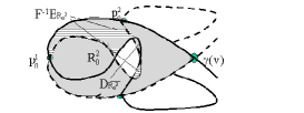
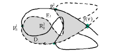
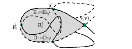
Figure 6. Exit sets and lobe.

For a general value of $N(\nu)$ (recall that $N(\nu)$ is even) we define the entering and exiting lobes as:

(9.6) $$D^{2k} =D^{2k-1}=\bigcup_{j=k+1}^{\frac{N(\nu)}{2}+k}D_{j}=\bigcup_{j=k+1}^{\frac{N(\nu)}{2}}D_{j}\cup\bigcup_{j=1}^{k}FD_{j},\ \ \$$

(9.7) $$\ E^{2k} =\bigcup_{j=k+1}^{\frac{N(\nu)}{2}+k}E_{j}=\bigcup_{j=k+1}^{\frac{N(\nu)}{2}}E_{j}\cup\bigcup_{j=1}^{k}FE_{j}$$

(9.8) $$\ E^{2k-1} =\bigcup_{j=k}^{\frac{N(\nu)}{2}+k-1}E_{j}=\bigcup_{j=k}^{\frac{N(\nu)}{2}}E_{j}\cup\bigcup_{j=1}^{k-1}FE_{j}$$

It follows (after some manipulation of (4.1)) that in the open geometry case (where $E_{i}\cap E_{j}=D_{i}\cap D_{j}=\emptyset$ for all $i\neq j$) the exit and entry sets of the regions $R_{0}^{r_{j}}$ are given by:

$$\begin{array}[c]{c}E_{R_{0}^{r_{j}}}=E^{j}\backslash\left(E^{j}\cap D^{j}\right)\\ D_{R_{0}^{r_{j}}}=F^{-1}\left(D^{j}\backslash\left(E^{j}\cap D^{j}\right)\right)\end{array}\text{ \ if \ }E_{i}\cap E_{j}=D_{i}\cap D_{j}=\emptyset\text{ \ for all }i\neq j.\text{\ \ \ \ \ \ \ \ \ }$$

In particular, in the near-integrable case, where $E^{j}\cap D^{j}=\emptyset$ for all $j=1,...,N(\nu)$ the exit and entry sets are given by the entering and exiting lobes. Indeed, for $N(\nu)=2$ we find:

$$D^{2}=D^{1}=FD_{1},\text{ \ }\ E^{1}=E_{1},E^{2}=FE_{1},$$

and therefore the first example follows this general rule.

9.3. Lobes in the adiabatic limit.

The limit of $\overline{\omega}(\nu)\rightarrow 0$ is called the adiabatic limit. It corresponds to a forcing with frequency which is much smaller than the time scale associated with the flow along the separatrix. The traditional way of analyzing this limit is by using the adiabatic approximation. In this approximation one considers solutions to the frozen Hamiltonian $H(x,y,\theta;0)=H_{0}(x,y;0)+H_{1}(x,y,\theta;0)$, namely the time-dependent oscillations are now fixed at the frozen phase $\theta$. One then studies adiabatic variables (to leading order, the action), and asserts that in the nonlinear case, as long as the solutions are bounded away from the separatrix, such variables cannot change by much due to the persistence of KAM tori. Furthermore, when the solution crosses the separatrix one can estimate the resulting change in the adiabatic invariances and the phases by constructing an adiabatic separatrix mapping (see for example [15],[21],[8],[7]). Another point of view which is applicable to the same limit (see [9],[10] and [20]), is concerned with the geometry of the manifolds and lobes. Consider the extended system $(x,y,\tau=\overline{\omega}(\nu)t)$, and realize that the manifold $\{(x,y,\tau)|x=x_{f},y=y_{f},\tau\in[0,2\pi)\}$ is a normally hyperbolic manifold for $\overline{\omega}(\nu)=0$, hence it persists with its stable and unstable manifolds for sufficiently small $\overline{\omega}(\nu)$. The solutions belonging to these manifolds can be well approximated, for semi-infinite time intervals by the extended system at $\overline{\omega}(\nu)=0.$ Denoting the homoclinic solution to this extended frozen system by $q_{h}(t;\tau_{0})=(x_{h}(t;\tau_{0}),y_{h}(t;\tau_{0}),\tau_{0})$ and the orbits belonging to the stable and unstable manifolds of the extended system by $q^{s,u}(t;\tau_{0},\nu)=(x^{s,u}(t;\tau_{0},\nu),y^{s,u}(t;\tau_{0},\nu),\tau=\overline{\omega}(\nu)t+\tau_{0})$ we see that as $\overline{\omega}(\nu)\rightarrow 0^{+}$

$$q^{s}(t;\tau_{0},\nu) =q_{h}(t;\tau_{0}+\overline{\omega}(\nu)t)+...,\text{ \ \ \ }t\in(-\infty,T]$$

$$q^{u}(t;\tau_{0},\nu) =q_{h}(t;\tau_{0}+\overline{\omega}(\nu)t)+...,\text{ \ \ \ \ }t\in[-T,\infty)$$

where dots stand for higher order terms in $\overline{\omega}(\nu)$, $T$ is a positive constant and the higher order terms are small for $\overline{\omega}(\nu)<$ $\omega^{\ast}(T)$. Recall that in the limit $\nu\rightarrow 0^{+}$ (which, by A3 corresponds to the limit $\overline{\omega}(\nu)\rightarrow 0^{+}$), there are $N(0^{+})$ topologically transverse primary homoclinic orbits, $p^{n}=p^{n}(t;\tau_{0}^{n},\nu),n=1,...,N(0^{+})$. By definition, these orbits belong to both $q^{s}(t;\tau_{0}^{n},\nu)$ and $q^{u}(t;\tau_{0}^{n},\nu)$ for some phase $\tau$, so that $q^{s}(0;\tau_{0}^{n},\nu)=$ $q^{u}(0;\tau_{0}^{n},\nu)$. We conclude that these phases, $\tau_{0}^{n}$, are given, to leading order in $\overline{\omega}(\nu),$ by the phases at which the area enclosed by the frozen homoclinic loop achieves its maxima or minima:

Lemma 3.

(Kaper and Kovacic) Let $\{\theta_{i}\}_{i=1}^{N(0^{+})}$ denote the $\theta$’s at the minima and maxima of the homoclinic loop area $\mu(R(\theta))$, where $\mu(R(\theta_{1}))=\max_{\theta}\mu(R(\theta))$, and $N(0^{+})\geq 2$. Then, as $\overline{\omega}(\nu)\rightarrow 0^{+}$, the primary homoclinic orbits $p^{n}(t;\tau_{0}^{n},\nu)\rightarrow q_{h}(t;\theta_{n}+\overline{\omega}(\nu)t)$ and:

$$\mu(R(\theta_{n}))=\mu(R_{0}^{n})+o(1)$$

where $R_{0}^{n}$ denotes the region enclosed by $U[\gamma,p^{n}]$ and $S[\gamma,p^{n}]$.

Proof.

See [10], where it is proved that to leading order the adiabatic Melnikov function, which measures the distance between the stable and unstable manifolds is given, to leading order, by $\frac{d}{d\theta}\mu(R(\theta)).$ ∎

Corollary 4.

As $\overline{\omega}(\nu)\rightarrow 0,$

$$\mu(E_{k}) =\mu(R(\theta_{2k-1}))-\mu(R(\theta_{2k}))$$

(9.9)

$$\mu(D_{k}) =\mu(R(\theta_{2k+1}))-\mu(R(\theta_{2k})),\text{ \ \ \ \ \ \ \ \ \ \ \ \ \ \ \ \ \ \ \ \ \ \ \ \ \ \ \ \ \ \ \ \ \ }$$

hence, provided A4 is satisfied

$$\mu_{E}(0^{+})=\lim_{\overline{\omega}(\nu)\rightarrow 0^{+}}\mu_{E}(\nu)=\sum_{k=1}^{\frac{N(0^{+})}{2}}\left(\mu(R(\theta_{2k-1}))-\mu(R(\theta_{2k}))\right)>0$$

The structure of the lobes in this limit is more complicated than the commonly seen graphs of homoclinic tangles. In particular, on one hand, generically, only one of the primary homoclinic points $p_{0}^{r_{n}}$ is bounded away from the fixed point $\gamma(\nu)$, leading to the creation of large lobes with area of $O(A)$ (see [9]). On the other hand the lobes get stretched and elongated, creating a web of small intersecting regions  (see [9],[4]).

Notice that if KAM tori exist, then the stable and unstable manifolds cannot intersect them, hence they are either interior or exterior to $R_{0}^{r_{k}}$

Lemma 4.

(Neishtadt [16]) Let $\theta_{n_{\min}}$ denote the phase at which $\mu(R(\theta))$ is minimal ($\mu(R(\theta_{n_{\min}}))=\min\mu(R(\theta)$). Then, as $\overline{\omega}(\nu)\rightarrow 0$, the area enclosed by the largest KAM torus inside $R_{0}^{r_{n}}$ (for any $n$), $\mu(R_{core}(\nu))$ asymptotes $\mu(R(\theta_{n_{\min}}))$:

$$\mu(R(\theta_{n_{\min}}))=\mu(R_{core}(\nu))+...$$

Furthermore, it is estimated in [16] that the error scales as $O(\overline{\omega}^{2}\left|\ln\overline{\omega}\right|^{2}).$

References

- [1] V. Arnold. Dynamical Systems, III, Encyclopedia of Mathematical Sciences. Springer-Verlag, Berlin, 1988.
- [2] S. Channon and J. Lebowitz. Numerical experiments in stochasticity and homoclinic oscillations. annals. NY Ac. Sc., 357:108–118, 1980.
- [3] R. Easton. Trellises formed by stable and unstable manifolds in the plane. Trans. Am. Math. Soc., 294:2, 1986.
- [4] Y. Elskens and D. Escande. Slowly pulsating separatrices sweep homoclinic tangles where islands must be small: An extension of classical adiabatic theory. Nonlinearity, 4:615–667, 1991.
- [5] V. Gelfreich. Melnikov method and exponentially small splitting of separatrices. Physica D, 101(3–4):227–248, Mar 1997.
- [6] J. Guckenheimer and P. Holmes. Non-Linear Oscillations, Dynamical Systems and Bifurcations of Vector Fields. Springer-Verlag, New York, NY, 1983.
- [7] R. Haberman, R. Rand, and T. Yuster. Resonant capture and separatrix crossing in dual-spin spacecraft. Nonlinear Dynam., 18(2):159–184, 1999.
- [8] J. Henrard. Capture into resonance: An extension of the use of adiabatic invariants. Celest. Mech., 27:3–22, 1982.
- [9] T. Kaper and S. Wiggins. Lobe area in adiabatic systems. In Nonlinear Science: The Next Decade, proc. CNLS 10th Annual Conf., Physica D.
- [10] T. J. Kaper and G. Kovačič. A geometric criterion for adiabatic chaos. J. Math. Phys., 35(3):1202–1218, 1994.
- [11] R. MacKay, J. Meiss, and I. Percival. Transport in Hamiltonian systems. Physica D, 13:55–81, 1984.
- [12] J. Meiss. Symplectic maps, variational principles, and transport. Rev. of Modern Phys., 64(3):795–848, 1992.
- [13] J. Meiss. Average exit time for volume preserving maps. Chaos, 7(1):139–147, 1997.
- [14] A. Neishtadt. The separation of motions in systems with rapidly rotating phase. P.M.M. USSR, 48:133–139, 1984.
- [15] A. I. Neishtadt. Passage through a separatrix in a resonance problem with a slowly-varying parameter. Prikl. Mat. Meh., 39(4-6):1331–1334, 1975.
- [16] A. I. Neĭshtadt, Chaĭkovskiĭ, and A. A. Chernikov. Adiabatic chaos and particle diffusion. Sov. Phys. JETP, 72(3):423–430, 1991.
- [17] H. Poincaré. Les Methods Nouvelles de la Mechanique Celeste. Gauthier-Villars, Paris, 1892.
- [18] V. Rom-Kedar and A. C. Poje. Universal properties of chaotic transport in the presence of diffusion. Phys. of Fluids, 11(8):2044–2057, 1999.
- [19] V. Rom-Kedar and S. Wiggins. Transport in two-dimensional maps. Archive for Rational Mech. and Anal., 109(3):239–298, 1990.
- [20] C. Soto-Trevinõ and T. J. Kaper. Higher-order melnikov theory for adiabatic systems. J. Math. Phys., 37(12):6220–6249, 1996.
- [21] J. L. Tennyson, J. R. Cary, and D. F. Escande. Change of the adiabatic invariant due to separatrix crossing. Phys. Rev. Lett., 56(20):2117–2120, 1986.
- [22] D. Treschev. Width of stochastic layers in near-integrable two-dimensional symplectic maps. Phys. D, 116(1-2):21–43, 1998.
- [23] D. Turaev. Polynomial approximations of symplectic dynamics and richness of chaos in non-hyperbolic area preserving maps. submitted preprint, 2002.