Spectral theory for the failure of linear control in a nonlinear stochastic system

Abstract

We consider the failure of localized control in a nonlinear spatially extended system caused by extremely small amounts of noise. It is shown that this failure occurs as a result of a nonlinear instability. Nonlinear instabilities can occur in systems described by linearly stable but strongly nonnormal evolution operators. In spatially extended systems the nonnormality manifests itself in two different but complementary ways: transient amplification and spectral focusing of disturbances. We show that temporal and spatial aspects of the nonnormality and the type of nonlinearity are all crucially important to understanding and describing the mechanism of nonlinear instability. Presented results are expected to apply equally to other physical systems where strong nonnormality is due to the presence of mean flow rather than the action of control.

It has been known for a long time that systems described by nonnormal evolution operators (operators with non-orthogonal eigenfunctions) often display rather surprising dynamics. For instance, turbulence in shear flows often develops for Reynolds numbers where the basic flow is still linearly stable. The critical Reynolds number was found to depend rather sensitively on the geometry of the system and the roughness of the boundaries. Several studies [1, 2, 3] have linked the onset of turbulence to a nonlinear instability arising from the interaction between the nonlinearity of the Navier-Stokes equation and the nonnormality of its linearization caused by significant mean flow. More recently the idea of a nonlinear instability has been used to explain the disagreement between the predictions of the linear stability analysis and experimental data for the contact line instability in gravity driven spreading of thin liquid films [4]. Nonnormality can also arise in the absence of mean flow as a result of localized feedback control [5, 6]. In this paper we use the idea of a nonlinear instability to explain the failure of localized control of a spatially extended nonlinear system in the presence of extremely weak noise. We extend and refine ideas described in [2, 5] by incorporating the information about the spatial degrees of freedom.

All studies of strongly nonnormal systems conducted up to now have analyzed the mechanism for nonlinear instability by concentrating only on the temporal dynamics. Although the importance of spatial degrees of freedom is generally recognized, the complexity of the problem usually prevents consistent spatiotemporal analysis. As the subsequent discussion shows, spatial information is crucial for understanding the mechanism that leads to nonlinear instability, which involves transient amplification of deviations produced by nonlinear terms. However, before developing the spatiotemporal description, it will be useful to review some results of the temporal analysis. Following [2] let us consider a system

$$\dot{\phi}=L\phi+f(\phi),$$ (1)

where $L$ is a stable linear operator and $f$ is a nonlinear function of its argument. In a purely linear system the disturbance decays asymptotically in time. However, if $L$ is nonnormal, this exponential decay can be preceded by a transient. The strength of nonnormality can be determined by the transient amplification factor

$$\gamma\equiv\max_{t,\phi(0)}\frac{\|\phi(t)\|}{\|\phi(0)\|}=\max_{t}\left\|e^{Lt}\right\|,$$ (2)

such that $\gamma=1$ for $L$ normal. The maximal transient amplification is achieved for the optimal initial disturbance $\phi(0)=\phi_{opt}$ at the optimal time $t=t_{opt}$ [7].

Any initial disturbance $\phi(0)$ with a nonvanishing component along $\phi_{opt}$ will be transiently amplified as well. For small disturbances, $\sigma=\|\phi(0)\|\ll 1$, the linear terms will dominate, so at the peak of the transient we will have $\|L\phi(t_{opt})\|\sim\|\phi(t_{opt})\|\sim\gamma\sigma$. For a quadratic nonlinearity, $\|f(\phi(t_{opt}))\|\sim(\gamma\sigma)^{2}$, so it will produce an integrated deviation in (1) of order $t_{opt}(\gamma\sigma)^{2}$ in the same amount of time it takes the linear operator to amplify the initial disturbance by $O(\gamma)$. The temporal analysis makes an implicit assumption that generically this deviation has again a nonvanishing component along the optimal disturbance $\phi_{opt}$, so it will be transiently amplified by $L$ in the same way as the initial disturbance. (As we will see below, this assumption can break down for spatially extended systems due to their high symmetry.) The deviation due to nonlinear terms will grow producing a positive feedback loop, if $t_{opt}(\gamma\sigma)^{2}\gtrsim\sigma$, and decay otherwise. The critical magnitude of a disturbance needed to bootstrap the nonlinear instability will, therefore, scale like $\sigma\sim t_{opt}^{-1}\gamma^{-2}$ for a quadratic nonlinearity. While in some systems like channel flow $t_{opt}\sim\gamma$, more often the dependence on $t_{opt}$ is too weak to be of any importance, e.g., for both coupled map lattices [5, 8] and partial differential equations [6] with localized control $t_{opt}\sim\log\gamma$. In the latter case we have a simple power law scaling $\sigma\sim\gamma^{\alpha}$ with an exponent $\alpha=-2$.

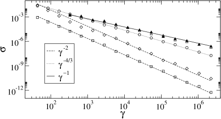
FIG. 1.: The noise level for which localized linear control fails as a function of the transient amplification factor for different types of nonlinearities ($\phi^{2}$ - squares, $\phi_{x}\phi$ - diamonds, $\phi^{3}$ - open triangles, $\phi^{4}$ - circles, $\phi^{5}$ - filled triangles). Straight lines are theoretical fits with slopes given by (5).

Sometimes, temporal analysis is sufficient and does give correct predictions for spatially extended systems. For instance, a controlled lattice of coupled quadratic maps [5] has indeed produced the scaling exponent $\alpha=-2$. However, sometimes the predictions of the temporal analysis are clearly wrong, suggesting that the spatial structure of disturbances plays an important role and cannot generally be ignored. A particularly simple example of the failure of temporal analysis is provided by the generalized Ginzburg-Landau equation (GGLE)

$${\phi}_{t}=\phi+\phi_{xx}+f(\phi)+\xi,$$ (3)

which (aside from the stochastic term $\xi$) is of the same form as (1). The dynamics of GGLE can be made linearly stable via feedback control imposed at the boundaries

$${\phi}(0,t)=0,\qquad\phi^{\prime}(L,t)=\int_{0}^{l}K(x)\phi(x,t)dx,$$ (4)

where $K(x)$ is an appropriately chosen gain function. As we have shown previously [6], the application of spatially localized control (4) to the spatially extended system (3) makes the linearized dynamics strongly nonnormal. We therefore expect the nonlinear instability to play a prominent role in destabilization as large transient amplification makes the dynamics extremely susceptible to noise. Numerical simulations of (3) with a power law nonlinearity $f(\phi)\propto\phi^{n}$ and random noise $\xi$ uniformly distributed on $(-\sigma,\sigma)$ show (see Fig. 1) that the critical noise level resulting in the failure of linear control scales as a power law $\sigma\sim\gamma^{\alpha}$, with an exponent well approximated by

$$\alpha=\left\{\matrix{-n/(n-1),&n=2,4,\cdots,\cr-1,\hfill&n=3,5,\cdots.}\right.$$ (5)

The exponent for $n$ even is correctly predicted by a properly generalized temporal analysis. Indeed, for controlled GGLE $t_{opt}\sim\log\gamma\sim l$, so comparing stochastic disturbances of order $\sigma$ with the distortions of order $(\gamma\sigma)^{n}$ produced by a combination of transient growth and nonlinearity, we immediately obtain the scaling $\sigma\sim\gamma^{-n/(n-1)}$. However, the corresponding exponent is inconsistent with our numerical results for $n$ odd.

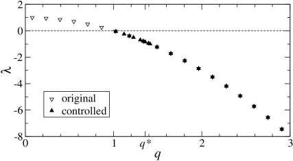
FIG. 2.: The wavenumbers $q_{n}$ and the corresponding eigenvalues $\lambda_{n}=1-q_{n}^{2}$ for the original and controlled system. The system size here and in the rest of the paper is $l=20$.

This discrepancy calls for the development of a more accurate theory that will be capable of explaining the effects of arbitrary types of nonlinearities. In particular, we would like to know why an advective term $\phi_{x}\phi$ produces the same scaling as a simple quadratic nonlinearity $\phi^{2}$ despite their different symmetry properties. As it turns out, the explanation can be obtained rather easily by conducting a spatiotemporal analysis of the bootstrapping mechanism. Indeed, transient amplification represents just one aspect of the nonnormal dynamics. The other aspect ignored by the temporal analysis is the focusing of the initial disturbances in the direction of the most strongly nonnormal eigenfunctions.

It is easy to see that due to the translational invariance of the linear operator $L=1+\partial_{x}^{2}$, its eigenfunctions are sinusoidal, with or without control. The boundary conditions (4) determine the wavenumber $q$ of an eigenfunction and the corresponding eigenvalue $\lambda=1-q^{2}$, such that the eigenfunction is stable when $q>1$ and unstable otherwise. In particular, the eigenfunctions of the original system (no feedback, $K(x)=0$) are $u_{k}(x)=\sin(q_{k}x)$ with $q_{k}=\pi(k-1/2)/l$, so at least one will be unstable for $l>\pi/2$. All eigenfunctions $v_{k}(x)=\sin(q^{\prime}_{k}x)$ of the controlled system are stable with wavenumbers $q^{\prime}_{k}>1$. In general, $q^{\prime}_{k}$ might be complex, but we can always force them to be real. This is done throughout the paper by calculating $K(x)$ using Linear-Quadratic control [9]. Appearance of complex eigenvalues does not affect the following analysis. As Fig. 2 shows, feedback (4) shifts all wavenumbers from the unstable band $Q_{+}=(0,1)$ into the stable band $Q_{-}=(1,\infty)$. The new wavenumbers $q^{\prime}_{k}$ cluster most tightly in a rather narrow band $Q_{\parallel}$ centered at $q^{*}\approx 1.36$. As the size $l$ of the system grows, an increasing number of eigenfunctions of the original system becomes unstable and gets squeezed into $Q_{\parallel}$ by feedback. As a result the distance between wavenumbers in $Q_{\parallel}$ shrinks and the corresponding eigenfunctions become increasingly aligned (nonnormal) [6].

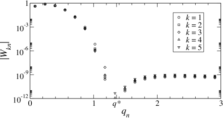
FIG. 3.: Fourier spectra of the first five adjoint eigenfunctions of the controlled system. The expansion is in the basis $\{u_{n}\}$ of eigenfunctions of the original system, $w_{k}(x)=\sum_{n}W_{kn}\sin(q_{n}x)$.

Now, let us consider what happens with an initial disturbance $\phi(x,0)$. Let us first concentrate on the linear effects. As the set $\{v_{k}\}$ is complete, in the absence of noise the general solution of the linearized equation (3) is given by

$$\phi(x,t)=\sum_{k=1}^{\infty}c_{k}v_{k}(x)\exp(\lambda^{\prime}_{k}t),$$ (6)

where $\lambda^{\prime}_{k}=1-(q^{\prime}_{k})^{2}$. The coefficients $c_{k}$ can be found using the adjoint eigenfunctions $w_{k}(x)$:

$$c_{k}=\frac{(w_{k}(x),\phi(x,0))}{(w_{k}(x),v_{k}(x))},$$ (7)

where we assume that the eigenfunctions are normalized such that $\|w_{k}\|=\|v_{k}\|=1$. As the eigenvalues $\lambda^{\prime}_{k}$ are all stable, it is clear that transient amplification can only result from large values of the coefficients $c_{k}$. For $c_{k}$ to become large two conditions have to be satisfied. First, the numerator in (7) should not be small, i.e., the initial disturbance should not be orthogonal to the adjoint eigenvector $w_{k}$. As adjoint eigenvectors satisfy the orthogonality condition $(w_{k},v_{m})=0$ for $k\neq m$, their Fourier spectra are localized to the unstable band $Q_{+}$ (see Fig. 3). Therefore, only disturbances with significant spectral content in $Q_{+}$ will be transiently amplified. (Such disturbances will grow indefinitely in the uncontrolled system; control makes this growth transient.) This is illustrated in Fig. 4 which shows the transient amplification for sinusoidal initial disturbances:

$$\beta(q)=\max_{t}\left.\frac{\|\phi(x,t)\|}{\|\phi(x,0)\|}\right|_{\phi(x,0)=\sin(qx)}.$$ (8)

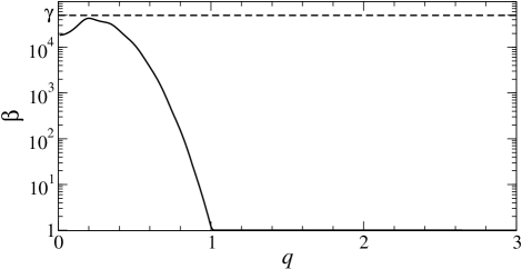
FIG. 4.: Transient amplification factor for sinusoidal initial disturbances as a function of their wavenumber.

The second condition is that the denominator in (7) should be small, which can only happen for strongly nonnormal eigenfunctions $v_{k}$ with $q^{\prime}_{k}\in Q_{\parallel}$. As a result, the Fourier spectrum of the transiently amplified disturbances will be strongly focused into the band $Q_{\parallel}$. This focusing effect can be clearly seen in Fig. 5 which shows the spectrum of the linearized GGLE driven by random noise. The spectrum is computed for the “worst case perturbation,” as this is the type of disturbance that leads to both the failure of linear control and more generally to the onset of nonlinear instability. Specifically, the state is expanded in the basis $\{v_{k}\}$

$$\phi(x,t)=\sum_{k=1}^{\infty}c_{k}(t)\sin(q^{\prime}_{k}x)$$ (9)

and the ”worst case” spectrum $F_{k}[\phi]$ is obtained by finding the maximal values of $|c_{k}(t)|$ for each $k$. The Fourier coefficients outside of $Q_{\parallel}$ are seen to be exponentially small. These two intimately related aspects of the nonnormal dynamics – transient amplification and focusing – are likely to be quite common in other strongly nonnormal spatially extended systems. For instance, a similar clustering of eigenfunctions is found in a model describing thermally driven spreading of liquid films [10].

Having understood the linear dynamics, let us now consider what happens when nonlinearities come into play. For sufficiently small $\sigma$ the nonlinearities will hardly change the linear dynamics. Their effect will be limited to “filtering” the transiently amplified disturbances, changing their magnitude and spectral content. As the transiently amplified disturbances have a very narrow spectrum, the spectrum of the signal produced by the nonlinear terms will also consist of several narrow peaks, as long as we consider nonlinearities of the power law type $f(\phi)=\phi^{n}$ with moderate $n$. (High powers are not interesting as the scaling exponents (5) for the even and odd powers become indistinguishable. Besides, most physically interesting nonlinearities have low powers.)

For instance, the spectrum of a quadratic nonlinearity, be it $\phi^{2}$ or $\phi_{x}\phi$, will only contain frequencies which are either sums or differences of frequencies $q^{\prime}_{k}$, i.e., 0, $|q^{\prime}_{m}-q^{\prime}_{n}|$, $2q^{\prime}_{m}$, and $q^{\prime}_{m}+q^{\prime}_{n}$. As the Fourier coefficient corresponding to the frequency $|q^{\prime}_{m}\pm q^{\prime}_{n}|$ is of order $c_{k}c_{m}$, the only significant contributions are produced when both $q^{\prime}_{m}$ and $q^{\prime}_{n}$ lie in $Q_{\parallel}$. This means that the spectrum of the quadratic term will be localized near $q=0$ and $q=2q^{*}$ (see Fig. 6a). The disturbances with $q\approx 2q^{*}$ are strongly damped, so the primary effect of most any quadratic nonlinearity will be to transfer the excitations from the band $Q_{\parallel}$ back into the band $Q_{+}$, where they will again be transiently amplified. After one full cycle involving transient amplification, focusing, and nonlinear filtering, an initial (e.g., stochastic) disturbance of order $\sigma$ will produce a deviation of order $(\gamma\sigma)^{2}$. Therefore, for $(\gamma\sigma)^{2}\gtrsim\sigma$ the low wavenumber disturbances will be driven predominantly by the nonlinear term, bootstrapping a nonlinear instability. A similar picture will be observed for $f(\phi)=\phi^{n}$ with $n=4,6,\cdots$. The spectrum of $f(\phi)$ will contain a strong component in $Q_{+}$ and the bootstrapping will occur for $(\gamma\sigma)^{n}\gtrsim\sigma$, so the critical noise will scale like $\gamma^{\alpha}$, with $\alpha$ given by (5).

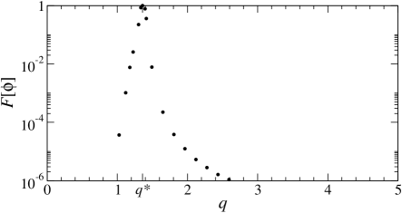
FIG. 5.: Normalized Fourier spectrum for a linear system driven by random noise uniformly distributed on $(-\sigma,\sigma)$.

The case of odd powers is substantially different. For instance, the spectrum of a cubic nonlinearity, $f(\phi)=\phi^{3}$, will only contain wavenumbers $|q^{\prime}_{m}\pm q^{\prime}_{n}\pm q^{\prime}_{k}|$. As the corresponding Fourier coefficients will be of order $c_{m}c_{n}c_{k}$, the spectrum will be strongly localized near $q=q^{*}$ and $q=3q^{*}$. Furthermore, as Fig. 6 shows, the spectral peaks of the nonlinear terms do not broaden. Therefore, a cubic nonlinearity will not transfer excitations from $Q_{\parallel}$ back to $Q_{+}$, and no bootstrapping will occur. The quintic nonlinearity, $f(\phi)=\phi^{5}$, is expected to produce similar results as its spectrum will be localized near $q^{*}$, $3q^{*}$, and $5q^{*}$, and so on. Destabilization will nevertheless occur for any power $n$ when the nonlinear terms become of the same order of magnitude as the linear terms, $(\gamma\sigma)^{n}\sim\gamma\sigma$, i.e., when $\gamma\sigma=O(1)$. At this point, the predictions of linear stability analysis become invalid. Therefore, for $n$ odd the critical noise will scale like $\gamma^{-1}$, justifying the second part of (5). The result for even powers is not changed, since nonlinear instability occurs for levels of noise much smaller than those at which linear stability analysis breaks down.

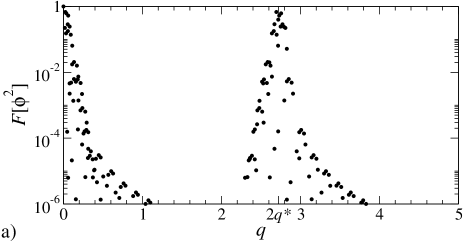
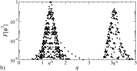
FIG. 6.: Normalized Fourier spectrum of (a) the quadratic term, $\phi^{2}$, and (b) the cubic term, $\phi^{3}$.

Summing up, we can conclude that, at least for a simple equation such as the stochastically driven GGLE studied here, the failure of localized control can be explained by a straightforward spectral analysis of transient dynamics. Moreover, spatiotemporal analysis appears to be crucial for understanding the mechanism of nonlinear instabilities in spatially extended systems in general. In particular, as the focusing effect described in this paper is an inherent feature of strongly nonnormal dynamics, its applicability is not constrained to the control problem considered here. A similar analysis could provide valuable insights into stability and control of shear flows, driven contact lines, and magnetic plasmas [11].

REFERENCES

- [1] K. M. Butler and B. F. Farrell, Phys. Fluids A 4, 1637 (1992)
- [2] L. N. Trefethen, A. E. Trefethen, S. C. Reddy, and T. A. Driscoll, Science 261, 578 (1993).
- [3] T. Gebhardt and S. Grossmann, Phys. Rev. E 50, 3705 (1994).
- [4] A. L. Bertozzi and M. P. Brenner, Phys. Fluids 9, 530 (1997); L. Kondic and A. L. Bertozzi, Phys. Fluids 11, 3560 (1999).
- [5] D. A. Egolf and J. E. S. Socolar, Phys. Rev. E 57, 5271 (1998).
- [6] R. O. Grigoriev and A. Handel, to be published by Phys. Rev. E, arxiv.org/abs/nlin.PS/0207023.
- [7] B. F. Farrell and P. J. Ioannou, J. Atmospheric Sci. 53, 2025 (1996)
- [8] R. O. Grigoriev, M. C. Cross, H. G. Schuster, Phys. Rev. Lett. 79, 2795 (1997).
- [9] P. Dorato, C. Abdallah and V. Cerrone, Linear-Quadratic Control (Prentice Hall, New Jersey, 1995)
- [10] R. O. Grigoriev, submitted to Phys. Fluids, arxiv.org/abs/nlin.PS/0207024
- [11] S. J. Camargo, M. K. Tippett, and I. L. Caldas, Phys. Plasma 7, 2849 (2000).