Abstract

We demonstrate, using the symbolic method together with p-adic and resultant methods, the existence of systems with exactly one or two generalized symmetries. Since the existence of one or two symmetries is often taken as a sure sign (or as the definition) of integrability, that is, the existence of symmetries on infinitely many orders, this shows that such practice is devoid of any mathematical foundation. Extensive computations show that systems with one symmetry are rather common, and with two symmetries are fairly rare, at least within the class we have been considering in this paper.

1 Introduction

In 1980 an observation was made at least twice by different authors. In [5] it is written

Another interesting fact regarding the symmetry structure of evolution equations is that in all known cases the existence of one generalized symmetry implies the existence of infinitely many.

and in [10] the same statement is made together with the footnote

This is not true for systems of equations. For example, the system $u_{t}=u_{2}+v^{2}/2,v_{t}=2v_{2}$ has a nontrivial group, but this group is exhausted by the one-parameter (with parameter $\tau$) group of transformations: $u_{\tau}=u_{3}+3vv_{1},v_{\tau}=4v_{3}$.

Here $v_{2}$ stands for $\frac{\partial^{2}v}{\partial x^{2}}$; we use the same notation in this paper. However, the ’counter-example’ given there is an integrable system, cf [1], section 3. In spite of this fact Fokas adapted the remark and formulated the following conjecture in 1987, [6].

Conjecture 1 (Fokas).

If a scalar equation possesses at least one time-independent non-Lie point symmetry, then it possesses infinitely many. Similarly for n-component equations one needs n symmetries.

Besides their mathematical interest, the observation and conjecture are of some practical importance since they are used to argue that it is enough to find only one or two symmetries of a system in order to declare it integrable, cf [13] and the discussion in [7]. This would be reasonable practice if it was simply not possible to prove integrability, but the methods employed in [15, 2, 16, 14, 17] showhow one can effectively obtain integrability proofs. Moreover, four years later Bakirov [1] published the first example of a non-integrable equation in the possession of a generalized symmetry. The system

$$\begin{array}[]{rll}u_{t}=&5u_{4}+v_{0}^{2}\\ v_{t}=&v_{4}\end{array}$$

has a sixth order symmetry

$$\begin{array}[]{rll}u_{t}=&11u_{6}+5v_{0}v_{2}+4v_{1}^{2}\\ v_{t}=&v_{6}\end{array}$$

as one can easily check. It was shown (with extensive computer algebra computations) that there are no other symmetries up to order 53. The authors of [2] proved in 1998 that the system of Bakirov does not possess another symmetry at any higher order, thereby proving that indeed one symmetry does not imply integrability. In [18] it is proved that there are in fact infinitely many fourth order systems with finitely many symmetries. The method used there could be used for seventh order systems as well and a system with two symmetries was found, a counterexample to Fokas’ conjecture. However for systems whose order is more than seven the approach can no longer be used. The method introduced here (using resultants) makes it possible to explore the symmetries of higher order systems.

2 The symmetry condition

We study symmetries of

$$\begin{array}[]{rll}u_{t}=&a_{1}u_{n}+K(v,v_{1},\ldots,v_{n-1})\\ v_{t}=&a_{2}v_{n}\end{array}$$

where $a_{1},a_{2}\in\mathbb{C}$ and $K$ is polynomial in $v(x,t)$ and its derivatives $v_{k}$. We call these ${\cal B}$–systems, where $n$ is the order of the system.

The right hand side of the equation can be interpreted as an element in a Lie algebra, the Lie bracket is computed using Fréchet derivatives as follows, see [12], [11]

$$.\begin{array}[b]{l}\left[\left(\begin{array}[]{c}{a_{1}u_{n}+K}\\ {a_{2}v_{n}}\end{array}\right),\left(\begin{array}[]{c}{b_{1}u_{m}+S}\\ {b_{2}v_{m}}\end{array}\right)\right]\\ \\ =\left(\begin{array}[]{cc}b_{1}D^{m}&D_{S}\\ 0&b_{2}D^{m}\end{array}\right)\left(\begin{array}[]{c}{a_{1}u_{n}+K}\\ {a_{2}v_{n}}\end{array}\right)-\left(\begin{array}[]{cc}a_{1}D^{n}&D_{K}\\ 0&a_{2}D^{n}\end{array}\right)\left(\begin{array}[]{c}{b_{1}u_{m}+S}\\ {b_{2}v_{m}}\end{array}\right)\\ \\ =\left(\begin{array}[]{c}{a_{1}D^{n}S-a_{2}D_{S}v_{n}-b_{1}D^{m}K+b_{2}D_{K}v_{m}}\\ {0}\end{array}\right).\end{array}$$ (1)

We call $S$ a symmetry of $K$ if $[K,S]$ vanishes. $K$ is called integrable when there exist symmetries on infinitely many orders and almost integrable when there exist symmetries on finitely many orders, cf. [18].

How to solve the equation $[K,S]=0$, given the order of $K$ and $S$? First of all, we see that if $K$ is polynomial, $S$ has to be polynomial too, cf. [1]. This enables us to use the symbolic calculus as developed in [8]. With the symbolic calculus the equation becomes polynomial and leads to divisibility conditions of certain elementary polynomials. These can be solved for infinitely many orders at once. The necessary and sufficient equations for the ratio of eigenvalues are obtained directly without having to specify the nonlinear part explicitly.

Assume that $K$ and $S$ are quadratic. A quadratic differential monomial is transformed into a symmetric polynomial in two symbols as follows

$$v_{i}v_{j}=\frac{\xi_{1}^{i}\xi_{2}^{j}+\xi_{1}^{j}\xi_{2}^{i}}{2}$$

The expression is symmetrized and divided by the number of symbol-permutations in order to ensure that

$$v_{i}v_{j}=v_{j}v_{i}$$

This procedure turns the operation of differentiation into ordinary multiplication

$$\begin{array}[]{ll}Dv_{i}v_{j}&=v_{i+1}v_{j}+v_{i}v_{j+1}\\ &=\frac{\xi_{1}^{i+1}\xi_{2}^{j}+\xi_{1}^{j}\xi_{2}^{i+1}+\xi_{1}^{i}\xi_{2}^{j+1}+\xi_{1}^{j+1}\xi_{2}^{i}}{2}\\ &=(\xi_{1}+\xi_{2})(\frac{\xi_{1}^{i}\xi_{2}^{j}+\xi_{1}^{j}\xi_{2}^{i}}{2}),\end{array}$$

like the action of the Fréchet derivative on a linear term

$$\begin{array}[]{ll}D_{v_{i}v_{j}}v_{k}&=v_{i+k}v_{j}+v_{i}v_{j+k}\\ &=\frac{\xi_{1}^{i+k}\xi_{2}^{j}+\xi_{1}^{j}\xi_{2}^{i+k}+\xi_{1}^{i}\xi_{2}^{j+k}+\xi_{1}^{j+k}\xi_{2}^{i}}{2}\\ &=(\xi^{k}_{1}+\xi^{k}_{2})(\frac{\xi_{1}^{i}\xi_{2}^{j}+\xi_{1}^{j}\xi_{2}^{i}}{2}).\end{array}$$

The symmetry condition for quadratic polynomials ($K,S\in\mathbb{C}[\xi_{1},\xi_{2}]$) reads

$$G_{n}[a_{1},a_{2}]S=G_{m}[b_{1},b_{2}]K$$

with the $G$–functions

$$G_{n}[a_{1},a_{2}](\xi_{1},\xi_{2})\stackrel{{\scriptstyle\mathrm{def}}}{{=}}a_{1}(\xi_{1}+\xi_{2})^{n}-a_{2}(\xi^{n}_{1}+\xi^{n}_{2})$$

If $G_{m}[b_{1},b_{2}]K$ is divisible by $G_{n}[a_{1},a_{2}]$ we have a symmetric polynomial expression for $S$ which can be transformed back. Because the $\xi_{1}$-degree of $K$ (the maximal number of x-derivatives of $u$ in the terms of $K$) is smaller than $n$, the function $G_{n}[a_{1},a_{2}]$ cannot divide $K$. Therefore $G_{n}[a_{1},a_{2}]$ should have a common factor with $G_{m}[b_{1},b_{2}]$ for there being a symmetry. Suppose we can find $a_{1},a_{2},b_{1},b_{2}\in\mathbb{C}$ such that ($F,L,T\in\mathbb{C}[\xi_{1},\xi_{2}]$)

$$\begin{array}[]{l}G_{n}[a_{1},a_{2}]=FL\\ G_{m}[b_{1},b_{2}]=FT.\end{array}$$

Then the Lie bracket (1) vanishes if one takes $K=LM$ and $S=MT$. One is free to choose $M\in\mathbb{C}[\xi_{1},\xi_{2}]$ as long as the $\xi_{1}$-degree of $K$ remains smaller than $n$. If this sounds a bit too easy, the reader should note that this determines the system and its symmetry at the same time, and does not say anything about hierarchies of symmetries.

3 The use of resultants

If the resultant of two polynomials vanishes, then their greatest common divisor has positive degree.

Lemma 1

Second order ${\cal B}$–systems have symmetries at all orders. The ratio of eigenvalues (and quadratic part) of the symmetries are fixed.

Proof.

Take $a_{1}\neq a_{2}$ again and $r\neq-1$. The $G$–function is

$$G_{2}[a_{1},a_{2}]=\frac{a_{1}-a_{2}}{r}(\xi_{1}-r\xi_{2})(r\xi_{1}-\xi_{2})\text{ with }(a_{2}-a_{1})r^{2}-2a_{1}r-(a_{2}-a_{1})=0,$$

and the resultant of $(\xi_{1}-r\xi_{2})$ with $G_{m}[b_{1},b_{2}]$ vanishes when

$$\frac{b_{1}}{b_{2}}=\frac{1+r^{m}}{(1+r)^{m}}.$$

With this ratio $(r\xi_{1}-\xi_{2})$ is a factor as well because the $G$–function is symmetric in $\xi_{1},\xi_{2}$ (the fraction $\frac{1+r^{m}}{(1+r)^{m}}$ is invariant under $r\rightarrow\frac{1}{r}$). ∎

This implies that to cover systems with finitely many symmetries the degree of the common factor of the $G$-functions should be higher than 2. Degree 3 is not enough because a third degree symmetric polynomial always contains the factor $\xi_{1}+\xi_{2}$. Their corresponding systems are always in a hierarchy of first, second or third order.

We look at factors of degree 4.

Lemma 2

The function $G_{n}[1+r^{n},(1+r)^{n}](\xi_{1},\xi_{2})$ has a factor of the form

$$(\xi_{1}-r\xi_{2})(r\xi_{1}-\xi_{2})(\xi_{1}-s\xi_{2})(s\xi_{1}-\xi_{2})$$

whenever $U_{n}\stackrel{{\scriptstyle\mathrm{def}}}{{=}}G_{n}[1+r^{n},(1+r)^{n}](1,s)=0$.

Proof.

The condition $U_{n}=0$ is expressing the fact that the ratio of eigenvalues of the $G$-function containing root $r$ equals the ratio of eigenvalues of the $G$-function containing root $s$. ∎

In the following we disregard the trivial factors of $U_{n}$ which are $(r-s)(rs-1)$ for all $m$ and $(r+1)(s+1)$ when $m$ is odd.

Lemma 3

Take $n>3.$ To obtain all eigenvalues of $n^{\text{th}}$ order ${\cal B}$-systems with a symmetry on order $m$ one calculates the resultant of $U_{n}$ and $U_{m}$ with respect to $s$ and applies the map $r\rightarrow\frac{1+r^{m}}{(1+r)^{m}}$ to its roots.

Proof.

If the resultant of $U_{n}$ and $U_{m}$ vanishes for some $r\in\mathbb{C}$ then by the previous Lemma $G_{n}[1+r^{n},(1+r)^{n}](\xi_{1},\xi_{2})$ and $G_{m}[1+r^{m},(1+r)^{m}](\xi_{1},\xi_{2})$ have a common fourth order factor. This implies that the $n^{\text{th}}$ order ${\cal B}$–system with eigenvalues $a_{1}=1+r^{n},a_{2}=(1+r)^{n}$ and quadratic part $G_{n}[a_{1},a_{2}]$ divided by this fourth order factor has a symmetry on order $m$. ∎

Example of Bakirov: The resultant of $U_{4}$ and $U_{6}$ with respect to $s$ contains the factor

$$f(r)=2r^{4}+10r^{3}+15r^{2}+10r+2.$$

We have that

$$1+r^{4}\text{ mod }f(r)\equiv 5\frac{r(2r^{2}+2+3r)}{-2}$$

and

$$(1+r)^{4}\text{ mod }f(r)\equiv\frac{r(2r^{2}+2+3r)}{-2}.$$

Their ratio is $5$, the ratio of the eigenvalues of the Bakirov system. As expected $G_{4}[5,1](1,r)$ is proportional to $f(r)$.

4 The use of p-adic numbers

The use of p-adic methods in integrability theory was initiated in [2]. For an introduction in p-adic number theory, see [9]. In this section we give a more expanded proof of the fact that the Bakirov system contains exactly one symmetry.

The p-adic field is notated by $\mathbb{Z}_{p}$ where $p$ is some prime number. Its elements are represented by series of the form $\sum_{n\geq 0}a_{n}p^{n}$ with coefficients $a_{n}\in\mathbb{Z}/p$. The p-adic expansion of an positive integer is just its base $p$ representation. For rational numbers we can get an infinite sequence. Examples: in $\mathbb{Z}_{5}$ we have

$$\begin{array}[]{l}57=2\cdot 5^{0}+1\cdot 5^{1}+2\cdot 5^{2}\\ \frac{3}{4}=1+\frac{1}{1-5}=2\cdot 5^{0}+\sum_{i=1}1\cdot 5^{i}.\end{array}$$

An element is invertible (in $\mathbb{Z}_{p}^{\times}$) if it is nonzero modulo $p$, that is: $a_{0}\neq 0$.

4.1 Hensels Lemma

The following lemma gives a method to check whether a polynomial has a root in $\mathbb{Z}_{p}^{\times}$.

Lemma 4 (Hensel)

A polynomial

$$f(r)=\sum_{i=0}^{m}c_{i}r^{i}\text{ with }c_{i}\in\mathbb{Z}_{p}$$

has a root in $\mathbb{Z}_{p}^{\times}$ if there exists an $\alpha_{1}\in\mathbb{Z}/p$ such that

• $f(\alpha_{1})\equiv 0\text{ mod }p$

• $\frac{df}{dr}(\alpha_{1})\not\equiv 0\text{ mod }p$.

Proof.

It is possible to construct a sequence {$\alpha_{n}$} with

$$\begin{array}[]{l}\alpha_{n}\text{ mod }p^{n-1}\alpha_{n-1}\\ f(\alpha_{n})\equiv 0\text{ mod }p^{n}\end{array}$$

Calculate $\beta\in\mathbb{Z}/p$ such that

$$0=f(\alpha_{n+1})=f(\alpha_{n}+\beta p^{n})\equiv f(\alpha_{n})+\frac{df}{dr}(\alpha_{1})\beta p^{n}\text{ mod }p^{n+1}.$$

By the induction hypotheses there exists a $\gamma\in\mathbb{Z}/p$ such that

$$f(\alpha_{n})\equiv\gamma p^{n}\text{ mod }p^{n+1}$$

Substituting this and dividing by $p^{n}$ gives an equation that can be solved in $\mathbb{Z}/p$:

$$\beta\equiv-\gamma(\frac{df}{dr}(\alpha_{1}))^{-1}\text{ mod }p.$$

Since the first step of the induction is part of the hypotheses, this concludes the proof. ∎

For example the square roots of 2 are in $\mathbb{Z}_{7}$. Take

$$f(r)=r^{2}-2$$

Then

$$\begin{array}[]{ll}f(3)\equiv 0\text{ mod }7,&f(4)\equiv 0\text{ mod }7\\ \frac{df}{dr}(3)\equiv 6\text{ mod }7,&\frac{df}{dr}(4)\equiv 1\text{ mod }7\end{array}$$

So Hensels Lemma can be applied. The number 3 is lifted as follows. Modulo $7^{2}$ we have

$$f(3)=1\cdot 7$$

so $\gamma=1$. The inverse of 6 in $\mathbb{Z}_{7}$ is 6. Then $\beta\equiv-1\cdot 6\equiv 1$. Indeed

$$f(3+1\cdot 7)=2\cdot 7^{2}$$

One step further gives

$$f(3+1\cdot 7+2\cdot 7^{2})=6\cdot 7^{3}+4\cdot 7^{4}$$

This shows that the method of Hensel is constructive.

4.2 The method of Skolem

Skolems method allows us to conclude that there exist only a finite number of symmetries. At first sight it looks a bit technical, but it is extremely powerful in our context. The method is based on the fact that if some equation does not have a solution in some p-adic field then it can not have a solution in $\mathbb{C}$. Moreover the method reduces the number of orders that need to be checked to a finite number.

If $x_{i}\in\mathbb{Z}_{p}^{\times}$ then by Fermats little theorem there exists a $y_{i}\in\mathbb{Z}_{p}$ such that $x_{i}^{p-1}=1+y_{i}p$. Let

$$u^{m}_{n}\stackrel{{\scriptstyle\mathrm{def}}}{{=}}\sum_{i=1}^{j}c_{i}y_{i}^{m}x_{i}^{n}$$

For instance, $U_{n}$, as defined in lemma 2, has the form of $u^{0}_{n}$ with $c_{i}=(-1)^{i}$ and $j=4$.

Lemma 5 (Skolem)

If $u^{0}_{k}\not\equiv 0$ mod $p$ then $\forall r,\ u^{0}_{k+r(p-1)}\neq 0$.

Proof.

$$u^{0}_{k+r(p-1)}=\sum_{i=1}^{j}c_{i}x_{i}^{k}(1+y_{i}p)^{r}\equiv u^{0}_{k}\text{ mod }p\neq 0.$$

Therefore $u^{0}_{k+r(p-1)}$ itself is $\neq 0$. ∎

Lemma 6 (Skolem)

If $u_{k}^{0}=0$ and $u^{1}_{k}\not\equiv 0$ mod $p$ then $\forall r>0$ we have $u^{0}_{k+r(p-1)}\neq 0$.

Proof.

Assume $u^{0}_{k+r(p-1)}=0$

$$0=\sum_{i=1}^{j}c_{i}x_{i}^{k}(1+y_{i}p)^{r}=\sum_{t=1}^{r}\left(\begin{array}[]{c}r\\ t\end{array}\right)p^{t}u^{t}_{k}$$

use

$$\frac{1}{r}\left(\begin{array}[]{c}r\\ t\end{array}\right)=\frac{1}{t}\left(\begin{array}[]{c}r-1\\ t-1\end{array}\right)$$

and divide by $pr$ to get

$$u^{1}_{k}+\sum_{t=2}^{r}\left(\begin{array}[]{c}r-1\\ t-1\end{array}\right)\frac{p^{t-1}}{t}u^{t}_{k}=0$$

This contradicts the second assumption since $\frac{p^{t-1}}{t}$ always contains a factor $p$. To see this write $t=p^{\alpha}s$ with $p\not|\ s$. Then $s$ is invertible and

$$\frac{p^{t-1}}{t}=\frac{1}{s}p^{p^{\alpha}s-\alpha-1}$$

The power of $p$ is bigger than 1 for when $\alpha=0$ we know $s\geq 2$ and when $\alpha\neq 0$ we have $s\geq 1$ and $p^{\alpha}\geq\alpha+2$ (because $p>2$). Hence we conclude $u^{0}_{k+r(p-1)}\neq 0$. ∎

With the lemmas of Skolem one has to search a prime number $p$ such that the $x_{i}$ are in the field $\mathbb{Z}_{p}^{\times}$, and check the conditions for finitely many orders ($p$-2). The computations one has to do are all modulo $p$ or $p^{2}$.

5 The Bakirov system

Here is how to use these lemmas for the Bakirov system. We let $p$ increase and look for p-adic roots of the resultant $2r^{4}+10r^{3}+15r^{2}+10r+2$. The first prime such that all conditions are satisfied is 181. In $\mathbb{Z}/181$ we find $f(66)=f(139)=0$. These numbers can be lifted to elements of $\mathbb{Z}^{\times}_{181}$. Modulo $p^{2}$ they are

$$r\equiv 66+13p,\ s\equiv 139+29p$$

The function $U_{m}(r,s)$ is has the form $u^{0}_{m}$ with $c_{i}=(-1)^{i}$, $j=4$ and

$$\begin{array}[]{l}x_{1}=1+s\equiv 140+29p\text{ mod }p^{2}\\ x_{2}=1+r\equiv 67+13p\text{ mod }p^{2}\\ x_{3}=r(1+s)\equiv 9+165p\text{ mod }p^{2}\\ x_{4}=s(1+r)\equiv 82\text{ mod }p^{2}\\ \end{array}$$

For $0\leq m<180$ we have $u^{0}_{m}(r,s)\equiv 0$ mod $p$ only when $m\in\{0,1,4,6\}$. Applying $x_{i}\rightarrow\frac{x_{i}^{p-1}-1}{p}$ gives

$$\begin{array}[]{l}y_{1}\equiv 40\text{ mod }p\\ y_{2}\equiv 33\text{ mod }p\\ y_{3}\equiv 140\text{ mod }p\\ y_{4}\equiv 46\text{ mod }p\end{array}$$

For $m\in\{0,1,4,6\}$ the function $u^{1}_{m}$

$$33\cdot 66^{m}+46\cdot 82^{m}-40\cdot 140^{m}-140\cdot 9^{m}$$

is nonzero modulo $p$. Both Skolems lemmas can be applied and it is shown that there is no non-trivial symmetry but at order 6.

6 The counter example to Fokas’ conjecture

Theorem 1

There exists a 2-component equation with exactly two non-trivial symmetries.

Proof.

The resultant of $U_{7}$ and $U_{11}$ has the following factor in common with the resultant of $U_{7}$ and $U_{29}$

$$(r^{3}-r-1)(r^{3}+r^{2}-1)(r^{6}+3r^{5}+5r^{4}+5r^{3}+5r^{2}+3r+1)$$

In $\mathbb{Z}/101$ the first factor has solution 20 and the third solution 52. These can be lifted and both Skolems lemmas can be applied. In this way it is proven that the set $\{r,\frac{1}{r},s,\frac{1}{s}\}$ that corresponds to the modulo $101$ set $S=\{20,96,52,68\}$ is no solution set of a $G_{m}$-function when $m\not\in\{0,1,7,11,29\}$. If one of the other sets corresponding to $\{40,48,42,89\}$ or $\{32,60,63,93\}$ is a solution set of the function $G_{m}$ for some $m$ then their minimum polynomials divides the resultant of $U_{7}$ with $U_{m}$. That means that $S$ is a solution set of $G_{m}$ as well, hence $m$ equals $0,1,7,11$ or $29$. ∎

We will compute the three equations and their symmetries explicitly. Each root of $r^{3}+r^{2}-1$ is mapped to a different eigenvalue. We take $\mathbb{C}[r]/(r^{3}+r^{2}-1)$ as our coefficient field. The eigenvalues of the systems will be

$$1+r^{7}=2r^{2}\text{ and }(1+r)^{7}=16r^{2}+28r+21$$

Their quadratic part will be

$$G_{7}[2r^{2},16r^{2}+28r+21](\xi_{1},\xi_{2})$$

divided by

$$2(\xi_{1}-r\xi_{2})(\xi_{1}-(r+r^{2})\xi_{2})(\xi_{1}^{2}+(1-r-r^{2})\xi_{1}\xi_{2}+\xi_{2}^{2})$$

i.e.

$$\frac{7}{2}(2r^{2}+4r+3)(\xi_{1}+\xi_{2})(\xi_{1}^{2}+(2-r)\xi_{1}\xi_{2}+\xi_{2}^{2})$$

Our examples, written more compactly than in [18], look like

$$\left.\begin{array}[]{rll}u_{t}=&2r^{2}u_{7}+7(2r^{2}+4r+3)(v_{3}v_{0}+(3-r)v_{2}v_{1})\\ v_{t}=&(16r^{2}+28r+21)v_{7}\end{array}\quad\right|r^{3}+r^{2}-1=0.$$

The symmetries can be calculated in the same way, leading to

$$\begin{array}[]{ll}u_{t}=&(-3r^{2}+r+2)u_{11}\\ &+11\left((14r^{2}+24r+18)v_{7}v_{0}+(35r^{2}+57r+42)v_{6}v_{1}\right.\\ &+\left.(48r^{2}+70r+49)v_{5}v_{2}+(51r^{2}+65r+42)v_{4}v_{3}\right)\\ v_{t}=&(151r^{2}+265r+200)v_{11}\end{array}$$

and

$$\begin{array}[]{ll}u_{t}=&(-40r^{2}+9r+17)u_{29}\\ &+29\left(30(1081r^{2}+1897r+1432)v_{25}v_{0}\right.\\ &+(311920r^{2}+547311r+413143)v_{24}v_{1}\\ &+(706832r+533441+403277r^{2})v_{23}v_{2}\\ &+(449543r^{2}+782050r+589257)v_{22}v_{3}\\ &+(537572r+402545+317304r^{2})/2v_{21}v_{4}\\ &+(1026233r^{2}+1635821r+1205570)v_{20}v_{5}\\ &+(1101516r+779787+787277r^{2})/2v_{19}v_{6}\\ &+(2656229r+1710194+2393075r^{2})v_{18}v_{7}\\ &+(3831912r^{2}+3208669r+1731205)v_{17}v_{8}\\ &+(6105788r^{2}+4007995r+1678107)v_{16}v_{9}\\ &+(4807604r+1421555+8899703r^{2})v_{15}v_{10}\\ &+(5263833r+11440843r^{2}+915604)v_{14}v_{11}\\ &+\left.3(1793035r+155000+4312473r^{2})v_{13}v_{12}\right)\\ v_{t}=&(3761840r^{2}+6601569r+4983377)v_{29}\end{array}$$

7 More symmetries

We present the results of large computer calculations we did in MAPLE [4]. We calculated the resultant of $U_{n}$ and $U_{m}$ for $4\leq n\leq 10$ and $n+1\leq m\leq n+150$. To obtain the systems with finitely many symmetries only, one has to filter out the integrable systems. How to find all integrable $n^{\text{th}}$ order systems for fixed $n$ if the quadratic part is $v_{0}^{2}$ is described in [3]. This method we have extended to cover the case of an arbitrary quadratic part. This will be the subject of another paper. One finds common factors on orders $m=k(n-1),kn,(2k+1)n$ for all $k\in\mathbb{N}$.

To give an indication of the size of the expressions. The resultant of $U_{10}$ and $U_{160}$ has degree $556$. The coefficients of $r^{n}$ with $244<n<312$ have 207 (decimal) digets. The number of $n^{\text{th}}$ order systems we have been calculating is

n	4	5	6	7	8	9	10	4–10
#	2745	2701	5679	5644	8740	8839	11952	46300

In the pictures on the next pages the positions of the roots of these resultants in the complex plane are plotted. As a fundamental domain the upper half unit circle is chosen. The full pictures are invariant under $r\rightarrow\frac{1}{r}$ and $r\rightarrow\bar{r}$.

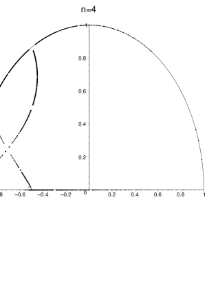
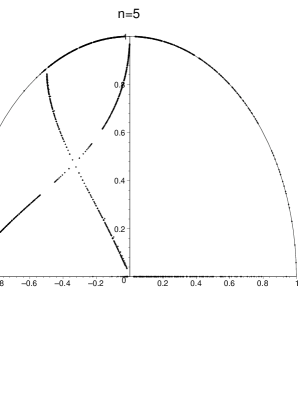
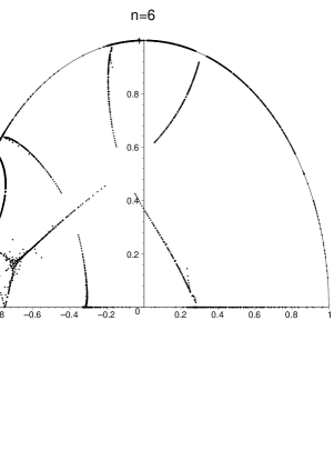
Figure 1: Numerical approximations of the roots of the $G$–functions corresponding to almost integrable systems for order $4,5$ and $6$

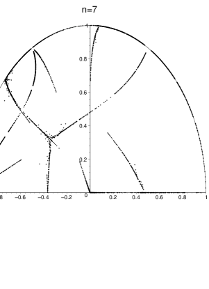
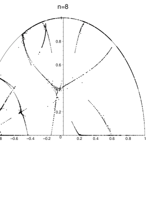
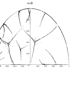
Figure 2: Numerical approximations of the roots of the $G$–functions corresponding to almost integrable systems for order $7,8$ and $9$

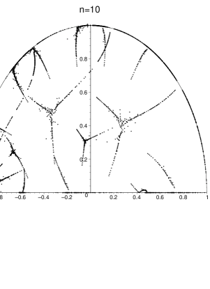
Figure 3: Numerical approximations of the roots of the $G$–functions corresponding to almost integrable systems for order $10$

All these systems have at least one nontrivial symmetry. To answer the question how many symmetries there exactly are we implemented the method of Skolem. We made the following refinements.

• Most of the resultants we have calculated are irreducible. By the argument in the proof of theorem 1 it suffices to prove the statement for one particular set of roots.

• Sometimes it is much more efficient to use two pairs of roots. The argument goes as follows. The resultant of $U_{5}$ and $U_{19}$ contains the factor

  $$\begin{array}[]{ll}f(r)=&r^{12}+4r^{11}+10r^{10}+19r^{9}+28r^{8}+34r^{7}\\ &+37r^{6}+34r^{5}+28r^{4}+19r^{3}+10r^{2}+4r+1\end{array}$$

  which is irreducible over $\mathbb{Q}$ and splits into linear factors over $\mathbb{Z}_{509}^{\times}$. The numbers $(264,407)$ are a solution for $U_{m}(r,s)$ when $m\in\{0,1,5,19,256,414\}$. The numbers $(267,300)$ are a solution for $U_{m}(r,s)$ when $m\in\{0,1,5,19,162,254\}$. By using both pairs we can apply lemma 5 for all $0\leq m<508$ but $\{0,1,5,19\}$, for which we can use the lemma 6. The computer could not find any prime such that the normal procedure works, it has been busy for days to check all primes $p<8147$.

With these improvements we have been able to prove that all these system have exactly one non trivial symmetry, with the exeption of the seventh order systems with two symmetries at order 11 and 29.

The following MAPLE output can be used to verify the above statement for $n=7,29\leq m\leq 37$.

prf29:=[101, {20, 52}],[97, {4, 32}]:
prf30:=[2531, {75, 871}]:
prf31:=[1021, {16, 42}]:
prf32:=[877, {226, 214}]:
prf33:=[601, {23, 409}]:
prf34:=[2857, {2457, 716}, {742, 391}]:
prf35:=[661, {401, 330}, {122, 245}]:
prf36:=[179, {17, 76}]:
prf37:=[233, {30, 56}, {20, 84}]:

The sequence prf.m contains the proofs for different factors of the resultant of $U_{7}$ and $U_{m}$. Each proof consists of a prime number $p$ and one or two sets of modulo $p$ solutions such that all conditions of Skolem are satisfied. The exceptions, where the resultant has two factors, are

$$(n,m)=(4,24),(4,28),(6,42),(7,8),(7,49),(8,56),(10,70)$$

Three factors appear at $n=7,m=11$ and four at $n=7,m=29$.

8 Conclusions

We have shown that the existence of one or two generalized symmetries of an evolution equation does not necessarily imply integrability. We hope that this illustrates the use of p-adic and resultant methods to this field and that these methods will be more widely applied. With these results in mind this puts a burden of proof on anyone claiming integrability (with respect to generalized symmetries). We mention the successful use of number theoretic methods, especially the Lech-Mahler theorem, in this respect, cf. [3, 17]. These methods are not restricted to the special kind of systems we study here, but they are applicable to any polynomial system, in principle.

References

• [1] Bakirov I M, On the Symmetries of Some System of Evolution Equations, Technical Report, 1991.
• [2] Beukers F, Sanders J A and Wang J P, One Symmetry does not Imply Integrability, J. Differential Equations 146 Nr.1 (1998), 251–260.
• [3] Beukers F, Sanders J A and Wang J P, On integrability of systems of evolution equations, J. of Differential Equations 172 Nr.2 (2001), 396–408.
• [4] Char B W, Geddes K O, Gonnet G H, Leong B L, Monagan M B and Watt S M, Maple V Language Reference Manual, Springer–Verlag, Berlin, 1991.
• [5] Fokas A S, A Symmetry Approach to Exactly Solvable Evolution Equations, J. Math. Phys. 21 Nr.6 (1980), 1318–1325.
• [6] Fokas A S, Symmetries and Integrability Stud. Appl. Math. 77 (1987), 253–299.
• [7] Foursov M V, On Integrable Coupled KdV-Type Systems, Inverse Problems 16 Nr.1 (2000), 259–274.
• [8] Gel’fand I M and Dikiĭ L A, Asymptotic Properties of the Resolvent of Sturm-Liouville Equations, and the Algebra of Korteweg-de Vries Equations, Uspehi Mat. Nauk 30 Nr.5(185) (1975), 67–100. English translation: Russian Math. Surveys 30 Nr.5 (1975), 77–113.
• [9] Gouvêa F Q, $p$-Adic Numbers. An introduction, Springer-Verlag, Berlin, second edition, 1997.
• [10] Ibragimov N H and Šabat A B, Evolution Equations with a Nontrivial Lie-Bäcklund Group, Funktsional. Anal. i Prilozhen. 14 Nr.1(96) (1980), 25–36.
• [11] Magri F, A Simple Model of Integrable Hamiltonian Equation, J. Math. Phys. 19 Nr.5 (1978), 1156–1162.
• [12] Olver P J, Applications of Lie Groups to Differential Equations, Volume 107 of Graduate Texts in Mathematics. Springer-Verlag, New York, second edition, 1993.
• [13] Olver P J and Sokolov V V, Integrable Evolution Equations on Associative Algebras, Comm. Math. Phys. 193 Nr.2 (1998), 245–268.
• [14] Olver P J and Wang J P, Classification of Integrable One-Component Systems on Associative Algebras, Proc. London Math. Soc. 81 Nr.3 (2000), 566–586.
• [15] Sanders J A and Wang J P, On the Integrability of Homogeneous Scalar Evolution Equations, J. Differential Equations 147 Nr.2 (1998), 410–434.
• [16] Sanders J A and Wang J P, On the Integrability of Non-Polynomial Scalar Evolution Equations, J. Differential Equations 166 Nr.1 (2000), 132–150.
• [17] Sanders J A and Wang J P, On the Integrability of Systems of Second Order Evolution Equations with Two Components, Technical Report WS–557, Vrije Universiteit Amsterdam, 2001. (Submitted to Journal of Differential Equations).
• [18] van der Kamp P H and Sanders J A, Almost Integrable Evolution Equations, Technical Report WS–534, Vrije Universiteit Amsterdam, 1999. (Submitted to Selecta Mathematica).