Singularities of Euler flow? Not out of the blue!

Abstract

Does three-dimensional incompressible Euler flow with smooth initial conditions develop a singularity with infinite vorticity after a finite time? This blowup problem is still open. After briefly reviewing what is known and pointing out some of the difficulties, we propose to tackle this issue for the class of flows having analytic initial data for which hypothetical real singularities are preceded by singularities at complex locations. We present some results concerning the nature of complex space singularities in two dimensions and propose a new strategy for the numerical investigation of blowup. (A version of the paper with higher-quality figures is available at http://www.obs-nice.fr/etc7/complex.pdf)

Dedicated to the memory of Richard Pelz.

I Phenomenology of blowup

According to Richardson’s ideas on high Reynolds number three-dimensional turbulence, energy introduced at the scale $\ell_{0}$, cascades down to a scale $\eta\ll\ell_{0}$ where it is dissipated. Consider the total time $T_{\star}$ which is the sum of the eddy turnover times associated with all the intermediate steps of the cascade. From standard phenomenology à la Kolmogorov 1941 (K41), the eddy turnover time varies as $\ell^{2/3}$. If we let the viscosity $\nu$, and thus $\eta$, tend to zero, $T_{\star}$ is the sum of an infinite convergent geometric series. Thus it takes a finite time for energy to cascade to infinitesimal scales, an observation first made by Onsager onsager49 . We also know that in the limit $\nu\to 0$, the enstrophy, the mean square vorticity, goes to infinity as $\nu^{-1}$ (to ensure a finite energy dissipation).

From such observations, it is tempting to conjecture that ideal flow, the solution of the (incompressible) 3-D Euler equation

$$\partial_{t}{\bm{v}}+{\bm{v}}\cdot\nabla{\bm{v}} = -\nabla p,$$ (1)

$$\nabla\cdot{\bm{v}} = 0,$$ (2)

when initially regular, will spontaneously develop a singularity in a finite time.

This is of course incorrect: the kind of phenomenology assumed above is meant only to describe the (statistically) steady state in which energy input and energy dissipation balance each other; the inviscid ($\nu=0$) initial-value problem is not within its scope. Another possible argument in favor of singularities has to do with the scaling properties of the high Reynolds number solutions (e.g. the $k^{-5/3}$ spectrum). For the simpler case of the Burgers turbulence houches81 , the scaling of spectra and structure functions is clearly rooted in the singularities (shocks) appearing in the solutions in the limit of vanishing viscosity. It is however well-known that power-law behavior can be present without any singularities. An example is the Holtsmark process, that is any component of the electric or gravitational field produced at a given point by a set of charges or masses with an initial Poisson distribution in space and moving with uniform independent isotropic velocities (having, e.g., a Gaussian distribution). It is then easily shown (by adaptation of the technique used by Chandrasekhar Chandrasekhar43 ) that the correlation function is $\propto|t-t^{\prime}|^{-1}$. This power-law behavior comes from the algebraic distribution of the distances of closest approach to the point of measurement and not from singularities of individual realizations (which are actually analytic).

There is yet another phenomenological argument, not requiring K41, which suggests finite-time blowup of the vorticity. Consider the equation for the vorticity ${\bm{\omega}}\equiv\nabla\wedge{\bm{v}}$ for inviscid flow, written as

$$D_{t}{\bm{\omega}}={\bm{\omega}}\cdot\nabla{\bm{v}},$$ (3)

where $D_{t}\equiv\partial_{t}+{\bm{v}}\cdot\nabla$ denotes the Lagrangian derivative. Observe that $\nabla{\bm{v}}$ has the same dimensions as $\bm{\omega}$ and can be related to it by an operator involving Poisson-type integrals. (For this use the fact that $\nabla^{2}{\bm{v}}=-\nabla\wedge\bm{\omega}$.) It is then tempting to predict that the solutions of (3) will behave as the solution of the scalar nonlinear equation

$$D_{t}s=s^{2},$$ (4)

which blows up in a time $1/s(0)$ when $s(0)>0$. Actually, (4) is just the sort of equation one obtains in trying to find rigorous upper bounds to various norms when studying the well-posedness of the Euler problem. This is precisely why the well-posedness ‘in the large’ (i.e. for arbitrary $t>0$) is an open problem in three dimensions.

The evidence is that the solutions of the Euler equation behave in a way much tamer than predicted by (4) because of a phenomenon known as “depletion of nonlinearity”: when small-scale structures appear through the nonlinear dynamical evolution from smooth initial data, they tend to display, at least locally, a much faster dependence on one particular spatial direction, so that the flow is to leading order one-dimensional frischetal83 . An example in three dimensions are the vorticity pancakes seen in simulations, as illustrated in Figure 1. If the flow were exactly one-dimensional, the nonlinearity would vanish (as a consequence of the incompressibility condition).

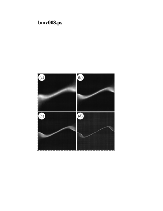
Figure 1: Simulation of the formation of a vorticity pancake at four different times from Ref. brachetetal92

Depending on how strong this depletion is and also on how persistent it is, finite-time blowup may or may not occur Frisch95 ; constantin-btl .

A review of the known mathematical results concerning the initial value problem for the Euler equation may be found in Ref. majda-bertozzi . We just mention a few salient facts. In two dimensions, for sufficiently smooth initial data in a bounded domain (including periodic boundary conditions) or with sufficiently fast decay at large distances, Hölder continuity of the vorticity is preserved for all times. The key result was actually obtained in 1933 wolibner ; holder . In three dimensions, for sufficiently smooth initial data, regularity is guaranteed only for a finite time. The first such result goes back to 1925 lichtenstein . A very important result, established in the late eighties by Beale, Kato and Majda (BKM) is that blowup, if it takes place, requires the time-integral of the supremum of the vorticity, and hence the vorticity itself, to become infinite bkm . As pointed out in Ref. majda-bertozzi , the main stumbling block in trying to improve the existing 3-D regularity results beyond a finite time is our still very rudimentary understanding of the mathematics of depletion. It is worth stressing here that an even partial progress on depletion could play a crucial role in understanding regularity issues for the 3-D Navier–Stokes equation claymath .

Numerical studies of 3-D blowup have been going on since at least the seventies with the development of spectral methods orszag-les-houches77 . The advantage of spectral methods is that they allow the kind of very high accuracy which is desirable in investigating possible singular behavior. When spectral methods were able to achieve fairly high resolutions ($256^{3}$ or more grid points), evidence for depletion emerged, possibly of sufficient strength to prevent blowup brachetetal (see also Section III). It was however realized that singularities (or near singularities) of the 3-D Euler are highly localized in space and that the kind of uniform grid used in standard spectral methods is very wasteful. A number of new methods were developed using nonuniform, e.g., adaptive meshing and often rather special initial conditions. Such studies have provided some evidence for blowup, based on extrapolating the behavior in time of the supremum of the vorticity. For the convenience of the reader we give a list of the key references (provided to us by R. Pelz and R. Kerr). It is not our purpose here to review such work.

We shall argue in this paper that there exists a class of analytic flows for which numerical studies of blowup can probably be carried out with sufficient control to distinguish genuine and spurious numerical blowup. In Section II, we recall some known facts about the Euler equation in the complex domain. In Section III, we first recall how to detect precursors of blowup by tracing complex space singularities with a spectral method; then we propose a new spectral adaptive approach capable, in principle, to resolve highly localized singularities. For this method it can be crucial to have information about the nature of complex space singularities. Sections IV and V report preliminary results concerning the singularities of the Euler equation in two space dimensions. Section VI presents concluding remarks.

II Analyticity of solutions to the Euler equation

We are here interested in solution of the $d$-dimensional Euler equation (2) with real analytic initial data ${\bm{v}}_{0}$, extended into the complex domain, a question addressed also in Refs. tanveer-speziale ; BNXW . For simplicity, we assume “periodic boundary conditions”, that is space periodicity with period 1 in all $d$ coordinates (although we use $2\pi$ when discussing numerical results). The configuration space is thus $\tilde{\mathbb{C}}^{d}\equiv{\mathbb{T}}^{d}+i{\mathbb{R}}^{d}$, where ${\mathbb{T}}^{d}$ is the $d$-dimensional periodicity torus. The analytic continuation of the solution to $\tilde{\mathbb{C}}^{d}$ is denoted ${\bm{v}}({\bm{z}},t)$, where ${\bm{z}}\equiv{\bm{x}}+i{\bm{y}}$ (we do not complexify the time variable).

We now give a brief survey of some key results for the Euler equation in the complex domain. Since this paper is intended mostly for a readership of fluid dynamicists, physicists and numerical analysts, we shall avoid using excessively formal mathematical language but, of course, distinguish clearly what is truly proven from what is just conjectured.

The first results about analyticity of the solution to the Euler equation have been obtained, to the best of our knowledge, in the seventies. With periodic boundary conditions, analyticity assumed initially, is preserved for all time in two dimensions bardos-benachour-zerner and at least for a finite time in three dimensions baouendi-goulaouic ; benachour76 . The simplest derivations of such results are obtained by using Lagrangian methods bardos-benachour ; benachour78 . One follows complex characteristics, the solutions of $\dot{\bm{z}}={\bm{v}}({\bm{z}},t)$, in order to control the width $\delta(t)$ of the “analyticity strip”, that is the distance from the real domain of the nearest singularity in $\tilde{\mathbb{C}}^{d}$ for the solution at time $t$.

What singles out two dimensions is that vorticity is conserved along the characteristics (as it is in the real domain). The key estimate used to prove all-time analyticity is that when $\delta(t)>s$ and $0<s<1$, one has

$$|{\rm Im}\,{\bm{v}}({\bm{x}}+i{\bm{y}},t)|\leq B_{s}||{\bm{\omega}}(\cdot,t)||_{s}\,|{\bm{y}}|\,\ln{1\over|{\bm{y}}|},$$ (5)

$$||{\bm{\omega}}(\cdot,t)||_{s}\equiv\sup_{|{\bm{y}}|\leq s,\,{\bm{x}}\in{\mathbb{T}}^{2}}|{\bm{\omega}}({\bm{x}}+i{\bm{y}},t)|,$$ (6)

where $B_{s}\equiv C_{1}+C_{2}\left(\ln(1/s)\right)^{-1}$ and $C_{1}$ and $C_{2}$ are positive constants. This is a consequence of the Biot–Savart law relating the velocity and the vorticity. Actually, (5) is mostly a reworking in the complex domain of an estimate obtained in Refs. wolibner ; holder for proving all-time regularity in the real domain. It follows from (5) and vorticity conservation that, if initially $\delta(0)>s$, at any later time the width of the analyticity strip has a double exponential lower bound $\delta(t)>s^{\exp(B_{s}||{\bm{\omega}}_{0}||_{s}t)}$. Hence analyticity holds for all times, but complex singularities can get arbitrarily close to the real domain.

In three dimensions, vorticity is not conserved since it can be stretched by velocity gradients. As a consequence, very poor control of $\delta$ is available and its vanishing after a finite time cannot be ruled out. Still, it is easy (but a bit technical) to show that, if at some time $t_{0}$ the solution is analytic, it will stay so in a (possibly small) time interval $[t_{0},t_{0}+T_{\star}[$. Furthermore it was shown by Benachour and Bardos that, if $\delta(t_{0})>s$ then, in this time interval, one has the square root lower bound $\delta(t)>(s/2)\left(1-(t-t_{0})/T_{\star}\right)^{1/2}$ benachour76 ; benachour78 ; bardos-benachour . One important consequence, is that: In three dimensions with periodic boundary conditions and analytic initial conditions, analyticity is preserved as long as the velocity is continuously differentiable ($C^{1}$) in the real domain bardos-benachour . The BKM theorem (cf. Section I) allows us to strengthening this result: analyticity is actually preserved as long as the vorticity is finite.

As long as $\delta>0$ the Euler equation can be written not only in the real domain but directly in the complex domain. In particular we shall find it useful to write it on “parareal domains”. By this we understand a domain of the form ${\mathbb{T}}^{d}+i{\bm{y}}$ for fixed ${\bm{y}}$ such that $|{\bm{y}}|<\delta$, i.e. obtained from the real (periodic) domain ${\mathbb{T}}^{d}$ by a fixed imaginary shift. In such a domain the velocity field is complex. By separating the velocity and the pressure into real and imaginary parts, ${\bm{v}}={\bm{v}}_{\rm r}+i{\bm{v}}_{\rm i}$ and $p=p_{\rm r}+ip_{\rm i}$, we can rewrite the Euler equation on a parareal domain as

$$\partial_{t}{{\bm{v}}_{\rm r}}+{{\bm{v}}_{\rm r}}\cdot\nabla{{\bm{v}}_{\rm r}}-{{\bm{v}}_{\rm i}}\cdot\nabla{{\bm{v}}_{\rm i}}=-\nabla p_{\rm r},$$ (7)

$$\partial_{t}{{\bm{v}}_{\rm i}}+{{\bm{v}}_{\rm r}}\cdot\nabla{{\bm{v}}_{\rm i}}+{{\bm{v}}_{\rm i}}\cdot\nabla{{\bm{v}}_{\rm r}}=-\nabla p_{\rm i},$$ (8)

$$\nabla\cdot{{\bm{v}}_{\rm r}}=0,\quad\nabla\cdot{{\bm{v}}_{\rm i}}=0.$$ (9)

Note that eqs. (7-9) have some similarity to the magnetohydrodynamics (MHD) equations, with ${\bm{v}}_{\rm r}$ and ${\bm{v}}_{\rm i}$ playing the role of the velocity field and the magnetic field, respectively. The main differences are the following: (i) the presence of a pressure term in the second equation (there is no such term in the MHD induction equation); (ii) if we linearize the equation around a uniform ${\bm{v}}_{\rm i}$, we do not obtain Alfvén-like waves but an instability whose growth rate is proportional to the wavenumber. The interpretation of this instability is that the imaginary translation induced by an imaginary velocity corresponds to an exponential factor in Fourier space (rather than a phase factor which would be associated to a real translation). We also observe that a real-imaginary decomposition similar to (7)-(9) has been used in Ref. grujic-kukavica for the Navier–Stokes equation in the complex domain (in order to estimate the space analyticity radius of solutions in terms of $L^{p}$ and $L^{\infty}$ norms of initial data).

The proof of the local-in-time analyticity result of Ref. baouendi-goulaouic is easily extended to the Euler equation in a parareal domain with analytic initial data in both two and three dimensions. All-time analyticity is now ruled out, even in two dimensions, since complex space singularities will generally cross after a finite time any parareal domain as they approach the real domain.

A consequence of local-in-time analyticity is that the width of the analyticity strip $\delta(t)$ cannot decrease discontinuously in time. This is a consequence of the Benachour–Bardos square root lower bound on $\delta(t)$ given above. In particular if there is finite-time blowup, that is $\delta(t)$ vanishes at some $t_{\star}$, the vanishing takes place continuously: real singularities do not come out of the blue (but out of the complex). This observation has led to the introduction of the method of tracing complex space singularities discussed in the next section.

Note that similar results about finite-time analyticity and continuity of $\delta(t)$ can be obtained without periodic boundary conditions, provided the solutions decrease sufficiently fast at large distances benachour78 . However, if the solutions are not well behaved at infinity the results may be wrong. A counterexample, due to S. Childress and E. Spiegel (quoted in rose-sulem ), is given by

$$\!\!\!\!\!\!\!\!{\bm{v}}(x_{1},x_{2},x_{3},t)=\left({x_{2}+x_{3}\over t-t_{\star}},{x_{3}+x_{1}\over t-t_{\star}},{x_{1}+x_{2}\over t-t_{\star}}\right),$$ (10)

$$\!\!\!\!\!\!\!\!p(x_{1},x_{2},x_{3},t)=-{x_{1}^{2}+x_{2}^{2}+x_{3}^{2}\over(t-t_{\star})^{2}}.$$ (11)

III Tracing complex singularities

As suggested in Refs. tracing ; houches81 , when the initial data for the Euler equation are analytic (and periodic), it is possible to trace the temporal behavior of the width of the analyticity strip $\delta(t)$ in order to obtain evidence for or against blowup. This takes advantage of the signature of complex space singularities in Fourier space. In one dimension, it is well known that an analytic function having isolated singularities in the complex plane has a Fourier transform whose modulus decreases at large wavenumbers $k$ as $\exp(-\delta k)$ (up to algebraic prefactors), where $\delta$ is the distance from the real domain of the nearest complex space singularity carrier-krook-pearson ; frisch-morf .

So far, nothing was known concerning the nature of complex space singularities of the multi-dimensional Euler equation. In more than one dimension, singularities in the complex domain are never point-like. For example, it may be shown that for the $d$-dimensional (potential) inviscid Burgers equation with analytic initial data, the singularities in the complex domain (before shock formation) are on $(d-1)$-dimensional complex manifolds, a result which cannot be ruled out for the Euler equation. In Fourier space, consider wavevectors of the form ${\bm{k}}=k\hat{\bm{k}}$ where $\hat{\bm{k}}$ is unit vector of fixed direction. For fixed $t$, it may then be shown that, as $k\to\infty$, the modulus of the Fourier transform decreases as $\exp(-\delta(\hat{\bm{k}},t)k)$ where $\delta$ now depends on the direction. The width of the analyticity strip at time $t$ is then the minimum of $\delta(\hat{\bm{k}},t)$ over all directions.

The numerical tracing of complex singularities is easy if the Euler equation is integrated by a (pseudo-)spectral method gottlieb-orszag with enough spatial resolution to capture the exponential tails in the Fourier transforms. This method was applied for the first time to the three-dimensional Euler flow generated by the Taylor–Green initial conditions brachetetal

$$\left.\begin{array}[]{rl}\displaystyle v_{1}\!\!\!\!&\displaystyle=\,\sin x_{1}\cos x_{2}\cos x_{3},\\[6.88889pt] \displaystyle v_{2}\!\!\!\!&=\displaystyle\,-\cos x_{1}\sin x_{2}\cos x_{3},\\[6.88889pt] \displaystyle v_{3}\!\!\!\!&=\displaystyle\,0.\end{array}\right\}$$ (12)

The simplest is then to plot for various times the “energy spectrum” $E(k,t)$, that is the angle-averaged squared modulus of the Fourier transform of the velocity. By a steepest descent argument one has (up to algebraic prefactors) $E(k,t)\propto\exp(-\delta(t)k)$. This is illustrated in Figure 2, taken from Ref. brachetetal , giving for the first time evidence that the Taylor–Green vortex may actually not have any blowup since $\delta(t)$ appears to decrease exponentially in time. This behavior is observed reliably over an interval of time during which $\delta(t)$ decreases by about one decade. Later work, extending the simulations from a $256^{3}$ to a $864^{3}$ grid, have confirmed this behavior over a range of one and a half decade in $\delta$ (see Figure 3 taken from Ref. brachetetal92 ).

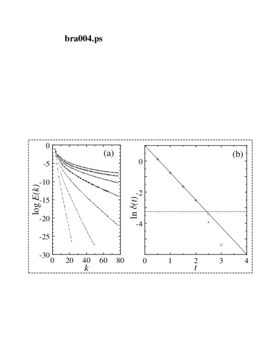
Figure 2: Spectral simulation of the inviscid Taylor–Green vortex using $256^{3}$ Fourier modes. (a) Evolution of the energy spectrum in lin–log coordinates; from bottom to top: output from time $t=0.5$ in increments of $0.5$. (b) Time-dependence of the width of the analyticity strip $\delta(t)$ in linear–log coordinates; the circles and plus signs correspond to $256^{3}$ and $128^{3}$ Fourier modes, respectively; the dashed line gives the threshold of reliability (from Ref. brachetetal ).

Figure 3: Width of the analyticity strip $\delta(t)$ from a spectral simulation of a periodic flow with no particular symmetry. Dashed line data are for $200^{3}$ modes and solid line data for $256^{3}$ modes (from Ref. brachetetal92 ).

The Taylor–Green vortex may just happen not to be a good candidate for blowup. It is special in at least two ways. First, it has a lot of symmetry (used to simplify the computation). Second, its vortex lines have non-generic topology: they are closed instead of displaying the KAM disorder that is typical of the integral lines of three-dimensional divergenceless vector fields. General periodic flow not displaying such pathologies has also been investigated in Ref. brachetetal92 . It seems to give exponential shrinking of $\delta$, but over just about half a decade in $\delta$. Two causes for this reduced range are clear: the limited resolution permitted ten years ago for flow without symmetry ($256^{3}$) and a crossover phenomenon between two different small-scale structures localized at different spatial locations, resulting into two different regimes with a changeover around $t=1.05$ (cf. Figure 3).

If we could simulate general periodic flow in such a way as to observe the variation of $\delta$ over several decades we would probably be able to get good evidence for or against blowup. One way to achieve this is just “patience”. We can indeed expect to gain a little more than a factor four in spatial resolution every ten years: this requires an increase in CPU power of $4^{4}=256$, made possible by Moore’s law. Another way is to renounce spectral methods and switch to adaptive methods. Unfortunately, such methods had so far only finite-order accuracy and could not be used to analytically continue the solutions into the complex domain, so that we must renounce measuring $\delta(t)$.

We propose here a new strategy, the “spectral adaptive” method which combines the highly localized refinement permitted by adaptive methods with full contact to the complex space structure. This method, which is still in the testing phase, will only be briefly outlined here. The basic idea is to run a standard spectral simulation until the latest time $t_{B}$ when $\delta(t)$ can be measured with very high accuracy and then to perform a “regularizing analytic transformation” $B$ on $\tilde{\mathbb{C}}^{3}$ with the following properties: (i) it preserves ${\mathbb{T}}^{3}$ globally and thus preserves periodicity, (ii) it maps the complex singularities of the solution at time $t_{B}$ away from ${\mathbb{R}}^{3}$ (possibly to complex infinity). In the new coordinates resulting from the transformation $B$, the problem is still periodic and can again be integrated by a suitable spectral method (with new difficulties since the coefficients are now strongly non-uniform). The procedure can, in principle, be repeated several times. The spectral adaptive strategy is yet to be fully implemented. So far, we have performed tests in one space dimension on the Burgers equation. These have revealed that, in order to minimize errors, it is best to perform the regularizing transformation around the time when the round-off noise just disappears from the tail of the spatial Fourier transform of the solution, which is a function of the resolution and of the round-off level (cf. Figure 4).

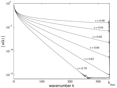
Figure 4: Evolution of the modulus of the Fourier transform for the solution of the one-dimensional Burgers equation with initial condition $u_{0}(x)=\sin x$, for which the first real singularity is at $t=1$. Around $t=0.82$ round-off noise disappears from the resolved spectral range. A rather moderate resolution of $1024$ modes is used in order to make the round-off noise fluctuations more visible.

For one-dimensional equations, complex singularities are point-like and we know simple transformations which have the required properties. In higher dimensions, singularities are on extended objects and their nature is not well known. A possible candidate for the regularizing analytic transformation $B$ could be the inverse Lagrangian map between time $t_{B}$ and the initial time (also called back-to-labels map constantin-btl ). This is definitely the case for the Burgers equation in any dimension, whose solution stays entire in Lagrangian coordinates if the initial condition is entire, that is analytic in the whole complex domain. However recent results for the two-dimensional incompressible Euler equation, the details of which will be published elsewhere, indicate that entire initial conditions develop complex-space singularities in both Eulerian and Lagrangian coordinates.

Note that the two-dimensional case is not just an academic problem, as one might infer incorrectly from the proven fact that 2-D Euler flow never blows up. One reason is that there is evidence that 2-D Euler flow is much tamer than predicted by the double exponential lower bound for $\delta(t)$ given in Section II. Indeed, spectral simulations indicate that $\delta(t)$ is actually decreasing exponentially tracing and that there is strongly depleted nonlinearity. Another reason is the existence of two-dimensional variants of the Euler equation for which blowup has still not been ruled out, such as axisymmetric flow with swirl or 2-D free convection GrauerSideris ; PumirSiggia_swirl ; EShu ; CaflischErcolaniSteele .

To find suitable candidates for the analytic transformation $B$ in two dimensions we would like to know something about the complex singularities of two-dimensional Euler flow with analytic initial conditions. This is the subject of the next section.

IV Numerical study of complex singularities for 2-D Euler flow

Spectral simulations of 2D Euler flow with analytic initial conditions give very strong evidence for the presence of complex space singularities through the presence of exponential tails in the Fourier transforms of the solution. Can we find out something about the nature of such singularities? One way is to analytically continue the solution at time $t$ to complex locations, using the Fourier series. Suppose we have the Fourier representation

$${\bm{v}}({\bm{x}},t)=\sum_{\bm{k}}{\rm e}^{i{\bm{k}}\cdot{\bm{x}}}\hat{\bm{v}}_{\bm{k}}(t),$$ (13)

we can just substitute ${\bm{z}}={\bm{x}}+i{\bm{y}}$ for ${\bm{x}}$ and obtain ${\bm{v}}({\bm{z}},t)$ as long as the series converges, that is for ${\bm{y}}<\delta(t)$. Alternatively, we can analytically continue the initial condition to the parareal domain ${\mathbb{T}}^{2}+i{\bm{y}}$ (a square in the 2D case) and then integrate the parareal equations (7)-(9) from $0$ to $t$. Mathematically, the two procedures are equivalent since they differ only by an imaginary translation, that is an overall exponential factor ${\rm e}^{-{\bm{k}}\cdot{\bm{y}}}$. Their numerical implementations in high-resolution spectral simulations may however not be equivalent, because of the presence of roundoff noise. At early times, when $\delta(t)$ can be quite large, the exponential falloff of the Fourier transform reaches roundoff noise level for wavenumbers which are much smaller than the maximum wavenumber permitted by the simulation (cf. Figure 5).

Figure 5: Angle average, at a given time, of the modulus of the Fourier transform of velocity in lin-log coordinates. The exponential falloff reaches here the roundoff noise level for wavenumbers of the order of 350, while the maximum wavenumber $k_{\max}$ determined by the $2/3$ dealiasing rule is 682 for a resolution of $2048^{2}$.

If we multiply this by the exponential factor ${\rm e}^{-{\bm{k}}\cdot{\bm{y}}}$, roundoff noise may be tremendously amplified (for ${\bm{k}}\cdot{\bm{y}}<0$). If we directly integrate in the parareal domain we can, at each time step, identify and set to zero the modes which are affected by roundoff, a procedure closely related to that used by Krasny for integration of the vortex sheet problem krasny . As $t$ increases, these modes will shift to higher wavenumbers, eventually reaching the maximum wavenumber permitted by the resolution. We are then effectively making better use of the available resolution. We call this procedure parareal integration with noise suppression. This method is rather crude and might be improved by taking into account the strong anisotropy present near a singularity.

We have used this method to integrate the two-dimensional parareal Euler equation using from $512^{2}$ to $2048^{2}$ modes and initial conditions which are trigonometric polynomials in the space coordinates and thus entire functions. (As we shall see later, such initial conditions are also amenable to a short-time expansion.) The cleanest results are obtained when the initial condition ${\bm{v}}_{0}({\bm{x}})$ has only two modes

$${\bm{v}}_{0}({\bm{x}})=(\partial_{2}\psi_{0}({\bm{x}}),\,-\partial_{1}\psi_{0}({\bm{x}})),$$ (14)

$$\psi_{0}({\bm{x}})=\cos(x_{1})+\cos(2x_{2}),$$ (15)

where $\psi({\bm{x}},t)$ is the stream function and $\partial_{1}$ and $\partial_{2}$ are the derivatives with respect to $x_{1}$ and $x_{2}$.

Figure 6: Snapshot of the contours of the real part of vorticity in the parareal domain $\bm{y}=(2\pi/64)(\cos\pi/6,-\sin\pi/6)$ just before the appearance of a singularity.

Figure 7: Enlargement of Figure 6 showing the contour lines of the real part of vorticity in the neighborhood of the location where the singularity appears.

Figures 6 and 7 show the real part of the vorticity $\omega\equiv-\nabla^{2}\psi$ at the latest time when the behavior in the parareal domain is still sufficiently smooth to be unaffected by truncation, that is when the complex singularities are not too close to the parareal domain chosen. It is seen that the solution in the near-singular region is almost one dimensional and hence has strongly depleted nonlinearity. The structure of the region of high vorticity gradients suggests that the singular set is a smooth curve. A cross section of the vorticity in the near-singular region is shown in Figure 8; a blowup of the region of highest vorticity (cf. Figure 9) shows about one decade of an approximately one-over-square root behavior (exponent $-1/2$) of the vorticity when crossing the singular manifold. This implies some range of square-root behavior for the velocity.

To check on errors due to truncation and filtering we changed the resolution from $512^{2}$ to $1024^{2}$ and $2048^{2}$ modes without changing any of the physical parameters (but, of course, adapting the time step to the spatial mesh). The results differed by less than the filtering level, a good indication of reliability. We also tried to extend the scaling range at the higher resolutions by chosing a slightly later output time, so as to let the singularities move closer to the parareal plane. In fact, the scaling range did not increase appreciably, perhaps because of roundoff problems. We cannot therefore ascertain that the vorticity truly diverges with exponent $-1/2$ when approaching the singular set.

Figure 8: Real and imaginary parts of vorticity along the cut represented as a dashed line on Figure 6. Both real and imaginary parts of vorticity display quasi-singular behavior near $s=-1.2$ and $s=0$.

Figure 9: Real part of the vorticity along the cut shown on Figure 8 in log-log coordinates. A range of algebraic behavior can be seen.

V Asymptotic analysis of 2-D complex singularities

In Ref. kuramoto the following result was established: the inviscid one-dimensional Burgers equation with initial conditions which are trigonometric polynomials in the space variable has, at short real times, square root branch point singularities for the velocity, which are within a distance $\delta(t)\propto\ln(1/t)$ of the real domain. It was also briefly pointed out that the $\ln(1/t)$ law can probably be extended to the 3-D Euler equation with initial conditions which are trigonometric polynomials in the space variables (such as the Taylor–Green flow). Further results on complex singularities for the Burgers equation may be found in Refs. bessisfournier84 ; bessisfournier90 .

We now show that the same law applies to the 2-D Euler equation at short times and, furthermore, we give a consistency argument shedding some light on the square root behavior reported in the previous section. For simplicity we shall limit ourselves to the two-mode initial condition (15) used in the previous section, although most of the arguments can be generalized to arbitrary trigonometric polynomials.

We start with the 2-D Euler equation written in stream function formulation

$$\partial_{t}\nabla^{2}\psi=J(\psi,\nabla^{2}\psi),$$ (16)

where $J(f,g)\equiv\partial_{1}f\partial_{2}g-\partial_{1}g\partial_{2}f$. It is easily shown that (16) has a solution in the form of a temporal Taylor series

$$\psi({\bm{x}},t)=\sum_{n\geq 0}\psi_{n}({\bm{x}})\,t^{n},$$ (17)

where $\psi_{0}$ is the initial condition and the $\psi_{n}({\bm{x}})$’s for $n\geq 1$ are defined recursively by

$$\nabla^{2}\psi_{n+1}=\frac{1}{n+1}\sum_{m+p=n}J(\psi_{m},\nabla^{2}\psi_{p}).$$ (18)

For the two-mode initial condition $\psi_{0}({\bm{x}})=\cos(x_{1})+\cos(2x_{2})$, it is easily checked that $\psi_{n+1}$ is a trigonometric polynomial which, when written in terms of complex exponentials, involves only modes of the form ${\rm e}^{ipx_{1}+2iqx_{2}}$ where $p$ and $q$ are signed integers such that $|p|+|q|\leq n+1$. Each term can now be continued from real ${\bm{x}}$ to complex ${\bm{z}}={\bm{x}}+i{\bm{y}}=(z_{1},\,z_{2})$.

Trigonometric polynomials are instances of entire functions. Hence, initially, $\delta=\infty$ and, by continuity, $\delta(t)$ will be large at small real times. Singularities will thus be present only for suitably large $|{\bm{y}}|$. For large positive $y_{1}$ and $y_{2}$, the dominant contributions to $\psi_{n}({\bm{x}}+i{\bm{y}})$ have $p<0$ and $q<0$. (For our special choice of initial conditions, symmetry arguments make it unnecessary to examine the other three sign quadrants in the ${\bm{y}}$ plane.) When $y_{1}\to+\infty$ and $y_{2}\to+\infty$, the dominant terms in $\psi_{n}({\bm{z}})$ are of the form

$$\psi_{n}({\bm{z}})\simeq\sum_{k=1}^{n}\beta^{n}_{k}{\rm e}^{-i\left[kz_{1}+2(n+1-k)z_{2}\right]},$$ (19)

where the complex coefficients $\beta^{n}_{k}$ satisfy suitable recursion relations, not needed here. If we formally keep only those dominant terms in (17), we obtain

$$\psi({\bm{z}},t) \simeq \frac{1}{2}\left({\rm e}^{-iz_{1}}+{\rm e}^{-2iz_{2}}\right)$$ (20)

$$+\frac{1}{t}\sum_{n\geq 0}\sum_{k=1}^{n}\beta^{n}_{k}\left(t{\rm e}^{-iz_{1}}\right)^{k}\left(t{\rm e}^{-2iz_{2}}\right)^{n+1-k}.$$

We now let $t\to 0$ and simultaneously $|{\bm{y}}|\to\infty$ in such a way that $t{\rm e}^{-iz_{1}}$ and $t{\rm e}^{-2iz_{2}}$ stay finite and we find that (i) all the terms in the Taylor expansion stay finite and (ii) all the terms not included in (20) are subdominant. This observation leads us naturally to making the asymptotic ansatz $\psi({\bm{z}},t)\simeq(1/t)F(\tilde{\bm{z}})$ where

$$\tilde{\bm{z}}=(\tilde{z}_{1},\,\tilde{z}_{2})\equiv(z_{1}+i\ln t,\,z_{2}+(i/2)\ln t).$$ (21)

Straightforward substitution into (16) leads to

$$\tilde{\nabla}^{2}(-1+i\tilde{\partial}_{1}+(i/2)\tilde{\partial}_{2})F=\tilde{J}(F,\tilde{\nabla}^{2}F),$$ (22)

where the overscript tilde means that the partial derivatives are taken with respect to the new variables. The initial condition (15) becomes now a boundary condition

$$F(\tilde{\bm{z}})\simeq\frac{1}{2}\left({\rm e}^{-i\tilde{z}_{1}}+{\rm e}^{-2i\tilde{z}_{2}}\right),\quad\tilde{y}_{1}\to-\infty,\,\,\,\,\tilde{y}_{2}\to-\infty.$$ (23)

If (22) with this boundary condition has a unique solution possessing complex space singularities at a finite distance from the real domain, then it follows immediately from the change of variables (21) that $\delta(t)\propto\ln(1/t)$ as $t\to 0$ in the original variables. We have recently checked numerically that, for the 2-D flow with initial condition given by (15), this scaling law holds over more than 8 decades, up to $t\approx 0.1$. Details will be published elsewhere together with numerical solutions of the asymptotic equation (22).

The numerical results of the previous section suggest that, for fixed $t$, the singularities in $\tilde{\mathbb{C}}^{2}$ are located on one-dimensional complex manifolds, near which the velocity has some range of square root behavior.

Using the short-time asymptotic equation (22), we show now that the observed behavior is consistent with the two-dimensional Euler equation. For this, assume that the (rescaled) stream function $F(\tilde{\bm{z}})$ can be represented, at least approximately, as

$$F(\tilde{\bm{z}})=G(\tilde{\bm{z}})+\Phi^{\alpha}(\tilde{\bm{z}})+{\rm h.o.t.},$$ (24)

where $G$ and $\Phi$ are analytic functions, $\alpha$ is a non-integer exponent, $\Phi$ (but not $G$) vanishes on the singular manifold ${\cal S}$ and h.o.t. stands for “higher order terms”, that is terms involving higher powers of $\Phi$. The expansion (24) is somewhat reminiscent of the singular expansion used in Refs. tanveer-speziale ; BNXW , except that (i) we do not a priori suppose that the singular manifold $\Phi=0$ moves with the flow and (ii) we shall determine the value of the exponent $\alpha$. Substituting (24) into (22), we obtain

$$\tilde{\nabla}^{2}(-1+i\tilde{\partial}_{1}+\frac{i}{2}\tilde{\partial}_{2})G-\tilde{J}(G,\tilde{\nabla}^{2}G)=$$

$$\gamma\left[(\tilde{\partial}_{1}\Phi)^{2}+(\tilde{\partial}_{2}\Phi)^{2}\right]\left[\tilde{J}(G,\Phi)-i(\tilde{\partial}_{1}+\frac{1}{2}\tilde{\partial}_{2})\Phi\right]\Phi^{\alpha-3}$$

$$+\alpha^{2}(\alpha-1)\tilde{J}(\Phi,(\tilde{\partial}_{1}\Phi)^{2}+(\tilde{\partial}_{2}\Phi)^{2})\Phi^{2\alpha-2}+{\rm h.o.t.},$$ (25)

where $\gamma\equiv\alpha(\alpha-1)(\alpha-2)$. In (25) the most singular term near ${\cal S}$ is that involving $\Phi^{\alpha-3}$, which cannot be balanced by any other term. Hence, its coefficient must vanish, thereby constraining the functions $G$ and $\Phi$ to satisfy $\tilde{J}(G,\Phi)-i(\tilde{\partial}_{1}+\frac{1}{2}\tilde{\partial}_{2})\Phi=0$. For non-integer $\alpha$, the term involving $\Phi^{2\alpha-2}$ also cannot be balanced by any other term unless it is actually analytic, that is $2\alpha-2$ is an integer. The smallest possible value is $\alpha=3/2$. The velocity has then exponent $1/2$, that is a square root behavior near ${\cal S}$. This is here derived under the assumption that $\Phi$ vanishes linearly near the singular manifold. Otherwise a different scaling law may be obtained.

VI Conclusion

It is clear that the issue of finite-time blowup is still open for initially smooth 3-D Euler flow (and also for 3-D Navier–Stokes flow). We have here proposed investigating this issue within the more restricted class of initially analytic flow, for which (hypothetical) real singularities are necessarily preceded by singularities in complex space. For this purpose we propose a new spectral adaptive strategy which requires the tracking of complex singularities and the use, at suitable times, of a regularizing map sending singularities too close to the real domain away from it.

Finally, we should mention that the issue of experimental study of 3-D Euler blowup was discussed at the workshop. We noted the following: if a flow is started by standard methods such as a moving grid, the “initial conditions” will have considerable small-scale excitation (viscous boundary layers generated at solid boundaries) and would in fact become singular if this was extrapolated to zero viscosity. Alternative ways may be tried where the flow is put in motion initially by body forces with no small-scale component, such as electromagnetic or (ultra)sonic stirring.

Acknowledgments

We are grateful to Claude Bardos and Peter Constantin for very useful discussions and remarks. Special thanks are due to Richard Pelz for many discussions and references; his recent untimely death is a great loss to us. Many thanks are also due to Robert Kerr for providing us with a number of references on blowup. Computational resources were provided by the Yukawa Institute (Kyoto). This research was supported by the Department of Energy, under contract W-7405-ENG-36, by the European Union under contract HPRN-CT-2000-00162, by the Indo-French Centre for the Promotion of Advanced Research (IFCPAR 2404-2), by the Japan Scholarship Foundation and by the Turbulence Working Group (Los Alamos).

References

- (1) L. Onsager, Statistical hydrodynamics, Nuovo Cimento 6(2), 279–287 (Suppl. Ser. IX) (1949).
- (2) U. Frisch, Fully developed turbulence and singularities, in Les Houches 1981: Chaotic Behavior of Deterministic Systems, G. Iooss, R. Hellemann and R. Stora eds., North-Holland, Amsterdam (1983).
- (3) S. Chandrasekhar, Stochastic problems in physics and astronomy, Rev. Mod. Phys. 15, 1–89 (1943).
- (4) U. Frisch, A. Pouquet, P.-L. Sulem and M. Meneguzzi, The dynamics of two-dimensional ideal MHD, J. Méc Théor. Appliqu. (Paris), 191–216 (Special issue on two-dimensional turbulence) (1983).
- (5) M.-E. Brachet, M. Meneguzzi, A. Vincent, H. Politano and P.-L. Sulem, Numerical evidence of smooth self-similar dynamics and possibility of subsequent collapse for three-dimensional ideal flows, Phys. Fluids 4, 2845–2854 (1992).
- (6) U. Frisch, Turbulence: the Legacy of A.N. Kolmogorov, Cambridge University Press, Cambridge (1995).
- (7) P. Constantin, An Eulerian–Lagrangian approach for incompressible fluids: local theory, J. Amer. Math. Soc. 14 263–277 (2000).
- (8) A.J. Majda and A.L. Bertozzi, Vorticity and incompressible flow, Cambridge Texts in Applied Mathematics, Cambridge University Press, Cambridge (2001).
- (9) W. Wolibner, Un théorème sur l’existence du mouvement plan d’un fluide parfait, homogène, incompressible, pendant un temps infiniment long, Math. Z 37, 698–726 (1933).
- (10) E. Hölder, Über die unbeschränkte Fortsetzbarkeit einer stetigen ebenen Bewegung in einer unbegretzen inkompressiblen Flüssigkeit, Math. Z 37, 727–738 (1933).
- (11) L. Lichtenstein, Über einige Existenzätze der Hydrodynamik homogener, unzusammendrückbarer, reibungsloser Flüssigkeiten und die Helmholtzschen Wirbelsätze, Math. Z 23, 89–154; 309–316 (1925)
- (12) J.T. Beale, T. Kato, and A.J. Majda, Remarks on the breakdown of smooth solutions for the 3-D Euler equations Commun. Math. Phys. 94 61–66 (1985).
-
(13)
C. Fefferman, Existence and smoothness of the
Navier-Stokes equations,
www.claymath.org/prizeproblems/navierstokes.htm (2000). - (14) S.A. Orszag, Statistical theory of turbulence, in Les Houches 1973: Fluid dynamics, R. Balian and J.L. Peube eds., Gordon and Breach, New York (1977).
- (15) M.-E. Brachet, D.I. Meiron, S.A. Orszag, B.G. Nickel, R.H. Morf and U. Frisch, Small-scale structure of the Taylor-Green vortex, J. Fluid. Mech. 130 411–452 (1983).
- (16) S. Tanveer and C.G. Speziale, Singularities of the Euler equation and hydrodynamic stability, Phys. Fluids A5, 1456–1465 (1993).
- (17) A. Bhattarcharjee, C.S. Ng and Xiaogang Wang, Finite-time singularity and Kolmogorov spectrum in a symmetric three-dimensional spiral model, Phys. Rev. E, 52, 5110–5123 (1995).
- (18) C. Bardos, S. Benachour and M. Zerner, Analyticité des solutions periodiques de l’équation d’Euler en deux dimensions, C. R. Acad. Sc. Paris 282 A, 995–998 (1976).
- (19) C. Goulaouic and M.S. Baouendi, Cauchy problem for analytic pseudo-differential operators, Comm. Partial Diff. Eq. 1, 135–189 (1976).
- (20) S. Benachour, Analyticité des solutions de l’équation d’Euler en trois dimensions, C. R. Acad. Sc. Paris 283 A, 107–110 (1976).
- (21) C. Bardos and S. Benachour, Domaine d’analyticité des solutions de l’équation d’Euler dans un ouvert de , Ann. Sci. Norm. Sup. Pisa 4, 647–687 (1977).
- (22) S. Benachour, Analyticity of solutions of Euler equations, Arch. Rat. Mech. Anal. 71 271–299 (1979).
- (23) Z. Grujic and I. Kukavica, Space analyticity for the Navier–Stokes and related equations with initial data in , J. Funct. Anal. 152, 447–466 (1998).
- (24) H.A. Rose and P.-L. Sulem, Fully developed turbulence and statistical mechanics, J. Phys. France 39, 441–484 (1978).
- (25) C. Sulem, P.-L. Sulem, and H. Frisch, Tracing complex singularities with spectral methods, J. Comput. Phys. 50, 138–161(1983).
- (26) G.F. Carrier, M. Krook and C.E. Pearson, Functions of a Complex Variable: Theory and Technique, McGraw-Hill, New York (1966).
- (27) U. Frisch and R. Morf, Intermittency in nonlinear dynamics and singularities at complex times, Phys. Rev. A 23, 2673–2705 (1981).
- (28) D. Gottlieb and S.A. Orszag, Numerical Analysis of Spectral Methods, SIAM, Philadelphia (1977).
- (29) R. Grauer & T.C. Sideris, Numerical computation of 3D incompressible ideal fluids with swirl Phys. Rev. Lett., 67 3511–3514 (1991). Finite time singularities in ideal fluids with swirl, Physica D, 88, 116–132 (1995).
- (30) A. Pumir & E. D. Siggia, Development of singular solutions to the axisymmetric Euler equations, Phys. Fluids A, 4 1472–1491 (1992).
- (31) W. E and C.-W. Shu, Small-scale structures in Boussinesq convection, Phys. Fluids, 6 49 (1994).
- (32) R.E. Caflisch, N. Ercolani and G. Steele, Geometry of Singularities for the Steady Boussinesq Equations, UCLA, CAM Report 95-22 (1995).
- (33) R. Krasny, A study of singularity formation in a vortex sheet by the point-vortex approximation, J. Fluid Mech. 167, 65–93 (1986).
- (34) U. Frisch, The analytic structure of turbulent flows, in Proceed. Chaos and statistical methods, Sept. 1983, Kyoto, Y. Kuramoto, ed. 1984, pp. 211-220, Springer.
- (35) D. Bessis and J.-D. Fournier, Pole condensation and the Riemann surface associated with a shock in Burgers’ equation, J. Phys. Lett. (Paris) 45, L833–L841 (1984).
- (36) D. Bessis and J.-D. Fournier, Complex singularities and the Riemann surface for the Burgers equation, in Nonlinear Physics, Proceedings of the International Conference, Shangai, April 24-30, 1989, Gu Chaohao, Li Yishen and Tu Guizhan eds., pp. 252–257, Springer, Berlin (1990). Additional references on Euler blowup
- (37) E. Behr, J. Necas and H. Wu, On blowup of solutions for Euler equations, Mathematical Modeling and Numerical Analysis 35, 229–238 (2001).
- (38) J.B. Bell and D.L. Marcus, Vorticity intensification and transition to turbulence in the three-dimensional Euler equations, Commun. Math. Phys. 147, 371–394 (1992).
- (39) M.-E. Brachet, Direct simulation of three-dimensional turbulence in the Taylor–Green vortex, Fluid Dyn. Res. 8, 1–8 (1991).
- (40) R.E. Caflisch and G.C. Papanicolaou Eds., Singularities in fluids, plasmas and optics, NATO Series C Vol. 404, Kluwer, Dordrecht (1993).
- (41) P. Constantin, Note on loss of regularity for solutions of the 3-D incompressible Euler and related equations, Commun. Math. Phys. 104, 311–329 (1986).
- (42) P. Constantin, Geometric statistics in turbulence, SIAM Rev. 36, 73–98 (1994).
- (43) P. Constantin, C. Fefferman, and A.J. Majda, Geometric constraints on potentially singular solutions for the 3-D Euler equations, Commun. Part. Diff. Eq. 21 (3-4), 559–571 (1996).
- (44) C.R. Doering and J.D. Gibbon, Applied analysis of the Navier-Stokes equations, Cambridge University Press, Cambridge (1995).
- (45) J.D. Gibbon and M. Heritage, Angular dependence and growth of vorticity in the three-dimensional Euler equations, Phys. Fluids 9, 901–909 (1997).
- (46) R. Grauer, C. Marliani and K. Germaschewski, Adaptive mesh refinement for singular solutions of the incompressible Euler equations, Phys. Rev. Lett. 80, 4177–4180 (1998).
- (47) T. Kato, Nonstationary flows of viscous and ideal fluids in , J. Funct. Anal. 9, 296–305 (1972).
- (48) R.M. Kerr, Evidence for a singularity of the three-dimensional incompressible Euler equations, Phys. Fluids A 5, 1725–1746 (1993).
- (49) J. Gibbon, B. Galanti and R.M. Kerr, Stretching and compression of vorticity in the 3-D Euler equations, in Turbulence structure and vortex dynamics, J.C.R. Hunt and J.C. Vassilicos Eds., Cambridge University Press, Cambridge (2000).
- (50) S. Kida, Three-dimensional periodic flows with high-symmetry, J. Phys. Soc. Japan 54, 2132–2136 (1985).
- (51) A.J. Majda, Vorticity, turbulence and acoustics in fluid flow, SIAM Rev. 33, 349–388 (1991).
- (52) C. Marchioro and M. Pulvirenti, The mathematical theory of incompressible nonviscous fluids, Springer, New York, 1991.
- (53) D.W. Moore, The spontaneous appearance of a singularity in the shape of an evolving vortex sheet, Proc. Roy. Soc. A 365, 105–119 (1979).
- (54) K. Ohkitani and J.D. Gibbon, Numerical study of singularity formation in a class of Euler and Navier–Stokes flows, Phys. Fluids 12, 3181–3194 (2000).
- (55) R.B. Pelz and O.N. Boratav, On a possible Euler singularity during transition in a high-symmetry flow, in Small-scale structures in three-dimensional hydro and magneto hydrodynamic turbulence, M. Meneguzzi, A. Pouquet and P.-L. Sulem Eds., Lecture Notes in Physics 462, Springer, Berlin, pp. 25–32 (1995).
- (56) R.B. Pelz, Symmetry and the hydrodynamic blow-up problem, J. Fluid Mech. 444, 299–320 (2001).
- (57) G. Ponce, Remark on a paper by J.T. Beale, T. Kato and A. Majda, Commun. Math. Phys. 98, 349–353 (1985).
- (58) G.I. Taylor and A.E. Green, Mechanism of the production of small eddies from large ones, Proc. Roy. Soc. A 158, 499–521 (1937).