Ray stability in weakly range-dependent sound channels

Abstract

Ray stability is investigated in environments consisting of a range-independent background sound-speed profile on which a range-dependent perturbation is superimposed. Theoretical arguments suggest and numerical results confirm that ray stability is strongly influenced by the background sound speed profile. Ray instability is shown to increase with increasing magnitude of $\alpha(I)=(I/\omega)\mathrm{d}\omega/\mathrm{d}I,$ where $2\pi/\omega(I)$ is the range of a ray double loop and $I$ is the ray action variable. This behavior is illustrated using internal-wave-induced scattering in deep ocean environments and rough surface scattering in upward refracting environments.

2002

205

5

Dated: ]

LABEL:FirstPage1

LABEL:LastPage#1102

identifier

I Introduction

Measurements made during the Slice89 propagation experiment Duda-et-al-92 , made in the eastern North Pacific, showed a clear contrast between highly structured steep ray arrivals and relatively unstructured near-axial flat ray arrivals. Measurements made during the AET experiment Worcester-et-al-99 ; Colosi-et-al-99 in a similar environment provided further evidence of the same behavior. Motivated by these observations, several authors Duda-Bowlin-94 ; Simmen-Flatte-Yu-Wang-97 ; Smirnov-Virovlyansky-Zaslavsky-01 have investigated ray sensitivity to environmental parameters. The work described in this paper continues the same line of investigation.

Like the earlier work we focus on ray path stability in physical space or phase space. The extension to travel time stability is not considered in this paper. Clearly, however, travel time stability must be addressed to fully understand the Slice89 and AET measurements. In spite of this limitation, and limitations of the ray approximation, our results are in agreement—qualitatively, at least—with the Slice89 and AET observations.

In Sec. II we provide the theoretical background for the work that follows. Most of this material builds on the action–angle form of the ray equations. A trivial observation that follows from the angle–action formalism is that ray sensitivity to the background sound speed structure is controlled by the function $\omega(I),$ where $2\pi/\omega$ is the range of a ray double loop and $I$ is the action variable. A heuristic argument suggests that $\mathrm{d}\omega/\mathrm{d}I$ should be closely linked to ray stability. In Sec. III we present numerical simulations that are chosen to demonstrate the importance of the background sound speed structure on ray stability. Simulations are shown for both internal-wave-induced scattering in deep ocean environments and rough surface scattering in upward-refracting environments. The latter are included to demostrate the generality of the arguments presented. These simulations strongly suggest that ray stability is controlled by the magnitude of the nondimensional quantity

$$\alpha(I)=\frac{I}{\omega}\frac{\mathrm{d}\omega}{\mathrm{d}I}.$$ (1)

In Sec. IV we explain the mechanism by which $\left|\alpha\right|$ controls ray stability. In Sec. V we summarize our results and briefly discuss: (i) the relationship between our work and earlier investigations; (ii) timefront stability; (iii) the dynamical systems viewpoint; and (iv) the extension to background sound speed structures with range-dependence. An appendix is reserved for some mathematical details.

II Theoretical background

A One-way ray equations

We consider underwater sound propagation in a two-dimensional waveguide with Cartesian coordinates $z$ (upward) and $r$ (along-waveguide). One-way ray trajectories satisfy the canonical Hamilton’s equations (cf. e.g. Ref. Brown-etal-03, and references therein),

$$\frac{\mathrm{d}p}{\mathrm{d}r}=-\frac{\partial h}{\partial z},\quad\frac{\mathrm{d}z}{\mathrm{d}r}=\frac{\partial h}{\partial p},$$ (2)

with Hamiltonian

$$h(p,z;r)=-\sqrt{c^{-2}-p^{2}}.$$

Here, $c(z;r)$ is the sound speed; $p$ is the vertical slowness which is understood as the momentum, conjugate to the generalized coordinate $z$; and $r$ is the independent (time-like) variable. The vertical slowness and the sound speed are related through $p\,c=\sin\varphi,$ where $\varphi$ is the angle that a ray makes with the horizontal.

B Near-integrability under small waveguide perturbations

Assume that the sound speed can be split as into a background (range-independent) part, $C(z),$ and a small range-dependent perturbation, $\delta c(z;r).$ Then, to lowest-order in $\delta c/c,$ the Hamiltonian takes the additive form

$$h=H(p,z)+\delta h(p,z;r).$$

Introduce now the Poincaré action

$$I=\frac{1}{2\pi}\oint\mathrm{d}z\,p=\frac{1}{\pi}\int_{z_{-}}^{z_{+}}\mathrm{d}z\,\sqrt{C^{-2}-H^{2}},$$ (3)

where $z_{\pm}$ denotes the vertical coordinate of the upper ($+$) and lower ($-$) turning points of a ray double loop, and consider the canonical transformation into action–angle variables $(p,z)\mapsto(I,\vartheta)$ defined by

$$p=\frac{\partial G}{\partial z},\;\vartheta=\frac{\partial G}{\partial I},\;G(z,I)=\int_{z_{-}}^{z}\mathrm{d}\xi\,\sqrt{C^{-2}(\xi)-H^{2}}.$$

According to the above transformation,

$$h(p,z;r)\mapsto\bar{H}(I)+\delta\bar{h}(I,\vartheta;r)$$

and the ray equations (2) take the form

$$\frac{\mathrm{d}I}{\mathrm{d}r}=-\frac{\partial}{\partial\vartheta}\delta\bar{h},\quad\frac{\mathrm{d}\vartheta}{\mathrm{d}r}=\omega+\frac{\partial}{\partial I}\delta\bar{h},$$ (4)

where

$$\omega(I)=\frac{\mathrm{d}\bar{H}}{\mathrm{d}I}.$$ (5)

Set (4) constitutes a near-integrable Hamiltonian system for the reasons explained next.

In the limit $\delta\bar{h}\rightarrow 0,$ the ray equations (4), which have one degree of freedom, are autonomous and the corresponding Hamiltonian, $\bar{H},$ is an integral of motion that constrains the dynamics. As a consequence, the equations are integrable through quadratures and the motion is periodic with (spatial) frequency $\omega$. Namely $I=I_{0}$ and $\vartheta=\vartheta_{0}+\omega r$ $\mathop{\mathrm{m}od}2\pi,$ where $I_{0}$ and $\vartheta_{0}$ are constants. Every solution curve is thus a line that winds around an invariant one-dimensional torus, whose representation in $(p,z)$-space is the closed curve given by the isoline $H=\bar{H}(I_{0}).$ Notice that $C^{-1}\cos\varphi=H;$ consequently, each torus can be uniquely identified by the ray axial angle defined by $\varphi_{a}(p,z)=\arccos C_{a}H$, where $C_{a}$ is the background sound speed at the sound channel axis.

With nonzero $\delta\bar{h}$, the Hamiltonian, $\bar{H}+\delta\bar{h},$ is no longer an invariant (the equations are nonautonomous) and the system may be sensitive to initial conditions, leading to chaotic motion in phase space. The distinction between regular and chaotic ray trajectories is commonly quantified by the Lyapunov exponent, formally defined by

$$\nu_{\infty}=\lim_{r\rightarrow\infty}\lim_{d_{0}\rightarrow 0}\frac{1}{r}\ln\frac{d}{d_{0}},$$ (6)

where $d(r),$ such that $d(0)=d_{0},$ is a suitably chosen measure of the separation between neighboring ray trajectories in phase space. For regular trajectories, $d\sim r^{a}$ as $r\rightarrow\infty$ with $a>0$ and, hence, $\nu_{\infty}=0.$ For chaotic trajectories, instead, $d\sim\exp\nu_{\infty}r$; in this case, $\nu_{\infty}^{-1}$, the average $\mathrm{e}$-folding range, is regarded as the predictability horizon.

C Variational equations

Although any norm of $(\delta p,\delta z),$ a perturbation to a trajectory $(p,z)$, could be used to define a distance in phase space, this is not a trivial task because $z$ and $p$ do not have the same dimensions, which complicates the evaluation of (6). The following procedure eliminates this problem.

The variational equations, which follow from the ray equations (2), are

$$\frac{\mathrm{d}\mathsf{Q}}{\mathrm{d}r}=\mathsf{JQ},\quad\mathsf{Q}(0)=\mathsf{I},$$ (7)

where

$$\mathsf{J}=\left[\begin{array}[]{cc}-\dfrac{\partial^{2}h}{\partial p\partial z}&-\dfrac{\partial^{2}h}{\partial z^{2}}\\ \dfrac{\partial^{2}h}{\partial p^{2}}&\dfrac{\partial^{2}h}{\partial p\partial z}\end{array}\right],\quad\mathsf{Q}=\left[\begin{array}[]{cc}\dfrac{\partial p}{\partial p_{0}}&\dfrac{\partial p}{\partial z_{0}}\\ \dfrac{\partial z}{\partial p_{0}}&\dfrac{\partial z}{\partial z_{0}}\end{array}\right],$$

with $p_{0}=p(0)$ and $z_{0}=z(0),$ and $\mathsf{I}$ is the identity matrix. Here, $\mathsf{J}(r)$ and $\mathsf{Q}(r)$ are the Jacobian matrices of the Hamiltonian vector field and associated flow, respectively; the last is usually referred to as the stability matrix. Notice that $(\delta p,\delta z)^{\mathrm{T}}=\mathsf{Q}(\delta p_{0},\delta z_{0})^{\mathrm{T}}$ at the lowest-order in $(\delta p_{0},\delta z_{0})$. Let now $\nu^{\mathsf{Q}}(r)$ be the largest of the two eigenvalues of $\mathsf{Q},$ and consider the definition (cf. e.g. Ref. Parker-Chua-89, )

$$\nu_{\infty}=\lim\limits_{r\rightarrow\infty}\dfrac{1}{r}\ln|\nu^{\mathsf{Q}}|\text{{.}}$$ (8)

If the limit in (8) exists, and is not nil, then $(\delta p,\delta z)\sim\exp\nu_{\infty}r$ as $r\rightarrow\infty$ (nearby trajectories diverge exponentially in range) and, hence, (8) can be taken as a suitable definition of the Lyapunov exponent. The equivalence between (6) and (8) can be understood by noting that the variational equations describe the evolution of an infinitesimal circle of initial conditions surrounding a specified ray initial condition. The circle gets deformed into an ellipse whose area equals that of the initial circle according to Liouville’s theorem (cf. e.g. Refs. Arnold-89, ; Tabor-89, ). The eigenvectors of Q define the orientation of the ellipse. The largest eigenvalue is a measure of the length of the semimajor axis and, hence, a suitable choice of $d.$

A simple but very important observation follows from the action–angle formalism. Dependence of the ray and variational equations on the background sound speed structure enters only through the function $\omega(I)$. The action–angle form of the variational equations for the perturbed system strongly suggests that ray stability and $\mathrm{d}\omega/\mathrm{d}I$ are closely linked. The mechanism through which $\mathrm{d}\omega/\mathrm{d}I$ influences ray stability can be seen from the action–angle form of the ray variational equations,

$$\frac{\mathrm{d}}{\mathrm{d}r}\delta I = -\dfrac{\partial^{2}\delta\bar{h}}{\partial I\partial\vartheta}\delta I-\dfrac{\partial^{2}\delta\bar{h}}{\partial\vartheta^{2}}\delta\vartheta,$$

$$\frac{\mathrm{d}}{\mathrm{d}r}\delta\vartheta = \dfrac{\mathrm{d}\omega}{\mathrm{d}I}\delta I+\dfrac{\partial^{2}\delta\bar{h}}{\partial I^{2}}\delta I+\dfrac{\partial^{2}\delta\bar{h}}{\partial I\partial\vartheta}\delta\vartheta.$$

If one assumes that the second derivatives of $\delta\bar{h}$ are zero-mean random variables, then when $\mathrm{d}\omega/\mathrm{d}I=0$ these terms should lead to slow (power-law) growth of $\delta\vartheta$ and $\delta I.$ But if $\left|\mathrm{d}\omega/\mathrm{d}I\right|$ is large, this term will cause $\left|\delta\vartheta\right|$ to rapidly grow for any nonzero $\left|\delta I\right|$. The perturbation terms will then lead to a mixing of $\left|\delta\vartheta\right|$ and $\left|\delta I\right|$. The term $\mathrm{d}\omega/\mathrm{d}I$ will lead, in turn, to further growth of $\left|\delta\vartheta\right|.$ As this process repeats itself, both $\left|\delta I\right|$ and $\left|\delta\vartheta\right|$ are expected to grow rapidly. Thus ray instability is expected to be significantly enhanced when $\left|\mathrm{d}\omega/\mathrm{d}I\right|$ is large.

D KAM theory

A (background) Hamiltonian is said to be nondegenerate if $\mathrm{d}\omega/\mathrm{d}I\neq 0$, i.e. if the frequency varies from torus to torus, which is a condition for nonlinearity of the system. An important result for near-integrable nondegenerate Hamiltonian systems is the celebrated Kolmogorov-Arnold-Moser (KAM) theorem on the stability of periodic solutions; cf. e.g. Refs. Arnold-89, ; Tabor-89, . This theorem states that if $\delta\bar{h}$ is small enough, for most initial conditions the motion remains periodic (i.e. confined to tori) and the complement of the periodic motion (i.e. the chaotic motion) has a measure that tends to zero as $\delta\bar{h}\rightarrow 0$. The KAM theorem thus guarantees that periodic motion (i.e. the KAM tori) separate the destroyed tori, leading to the notion of “islands” of (eternal) stability immersed in a chaotic “sea.”

The mechanism that produces the destruction of tori is trajectory–medium resonance; cf. e.g. Refs. Arnold-89, ; Tabor-89, . For example, assume the perturbation Hamiltonian $\delta\bar{h}$ to be periodic in range with frequency $\Omega$. Then it can be represented in Fourier series $\delta\bar{h}=\mathop{\mathrm{R}e}\sum_{m,n}A_{mn}(I)\exp\mathrm{i}(m\vartheta-n\Omega r)$. For KAM or nonresonant tori, $m\omega+n\Omega\neq 0$ for all integers $n,m$ and the motion is periodic. In contrast, those tori that satisfy $m\omega+n\Omega=0$ for some integers $n,m$ are said to be in resonance and chaotic motion develops. If several tori are captured into resonance, then the character of the chaotic motion will depend on whether these resonances overlap or not. For instance, consider two resonances centered at $I_{1}$ and $I_{2}.$ The widths of these resonances can be estimated as $\Delta I_{i}=4\sqrt{A_{i}/\left|\mathrm{d}\omega_{i}/\mathrm{d}I\right|}$, where $A_{i}$ is the amplitude of the resonant term in the above expansion. Define then $\Delta I=\Delta I_{1}+\Delta I_{2}.$ A benign form of chaos is present when these resonances are isolated, i.e. $\Delta I<|I_{1}-I_{2}|$; strong chaos, in contrast, emerges when these resonances overlap, i.e. $\Delta I>|I_{1}-I_{2}|$. The last criterion, due to Chirikov Chirikov-79 , gives thus a quantitative estimate of the size of the region of phase space occupied by chaotic trajectories.

The focus in KAM theory on the role of individual ray–medium resonances might seem to be at odds conceptually with the heuristic argument given at the end of the preceding subsection. There it was argued that the second derivatives of the perturbation to the environment could be treated as random variables. Ref. Brown-98, partially bridges this conceptual gap by showing that the KAM theorem can be applied to problems for which the perturbation consists of a superposition of an arbitrarily large finite number of frequencies. Chirikov’s criterion is still applicable, but its evaluation seems feasible only if the number of frequencies that comprises the perturbation is very small.

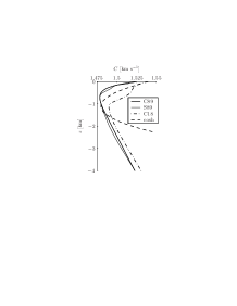
Figure 1: Background sound speed profiles used in the numerical work presented in this paper.

III Numerical simulations

In this section numerical simulations are presented which were chosen to demonstrate the importance of the background sound speed structure on ray stability. We consider first deep-water conditions and upward-refracting conditions afterward.

A Deep-water conditions

Four different background profiles are studied here (cf. Fig. 1). These are designated S89, C89, C18, and cosh. The S89 profile corresponds to a range average of the Slice89 sound speed observations. The C89 profile is a canonical profile Munk-74 with parameters chosen to approximately match S89’s sound channel axis depth, axial sound speed, and surface sound speed. The C18 profile can be regarded as an idealized model of the sound speed structure in the North Atlantic, whose upper ocean structure is associated with the $18\unit{{}^{\circ}{\mathrm{C}}}$ water mass Brown-etal-03 . Finally, the cosh profile, with cosh-dependence on depth relative to the axis, was chosen because it has the special property $\mathrm{d}\omega/\mathrm{d}I=0$ for all $I.$

The same internal-wave-induced sound speed perturbation field is superimposed on all four background profiles. This field is assumed to satisfy the relationship

$$\delta c/c=\mu N^{2}\zeta,$$ (9)

where $\zeta(z;r)$ is the internal-wave-induced vertical displacement of a water parcel and $N(z;r)$ is the Brunt–Väisälä frequency. Relationship (9) with $\mu=1.25\;\mathrm{\unit{s}}^{2}\mathrm{\unit{m}}^{-1}$ was found to give a good fit to AET hydrographic measurements Wolfson-Spiesberg-99 . Our simulated internal-wave-induced sound speed perturbations are similar to those used in Refs. Brown-etal-03, ; Beron-etal-02, ; these are based on Eq. (9) and make use of the $N$ profile estimated from measurements made during the AET experiment. The statistics of $\zeta$ are assumed to be described by the empirical Garrett–Munk spectrum Munk-81 . The vertical displacement $\zeta$ is computed using Eq. (19) of Ref. Colosi-Brown-98, with the variable $x$ replaced by $r$ and $y=0=t$. Physically this corresponds to a frozen vertical slice of the internal wave field that includes the influence of transversely propagating internal wave modes. A Fourier method is used to numerically generate the sound speed perturbation fields. A mode number cutoff of $30$ and a horizontal wavenumber cutoff of $2\pi$ $\unit{km}^{-1}$ were used in our simulations. The internal wave strength parameter was taken to be the nominal Garrett–Munk value.

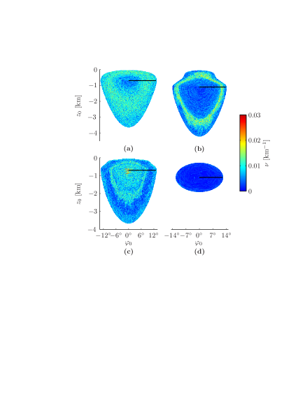
Figure 2: Stability exponents (finite range estimates of Lyapunov exponents) as a function of the initial depth and launch angle, for ray simulations in the (a) C89, (b) C18, (c) S89, and (d) cosh waveguides (cf. Fig. 1) with internal-wave-induced perturbations superimposed.

Fig. 2 shows the stability exponent, $\nu$ (a finite-range estimate of the Lyapunov exponent; cf. appendix A), as a function of initial ray position in phase space for each of the four environments considered. This figure provides a general picture of the ray motion stability character in each of the waveguides. In the C89 waveguide, ray trajectories with small (resp., large) unperturbed ray axial angles have small (resp., large) associated stability exponents. This trend is reversed in the S89 waveguide. The disparity in the stability properties of the ray motion in these waveguides contrasts with the close similarity of the corresponding background sound speed profiles. In the C18 waveguide ray trajectories have in general relatively small associated stability exponents, except in a narrow band of initial actions (or unperturbed axial angles) where the exponents are large and the ray motion more unstable. In opposition to the other waveguides, in the cosh profile the stability exponents are very small everywhere in phase space and the ray motion is remarkably stable.

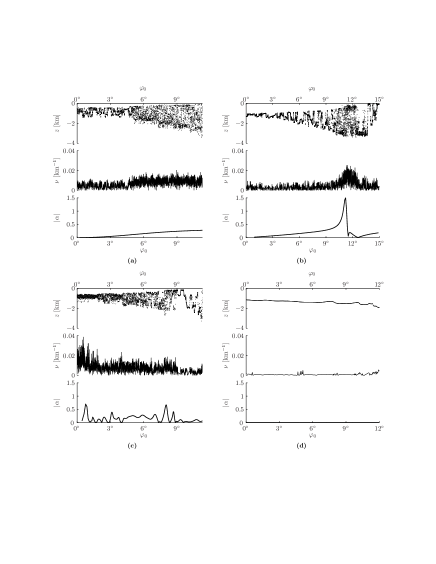
Figure 3: Each panel shows ray final depth (upper-plot), stability exponent (middle-plot), and stability parameter (lower-plot) at $1000$ $\unit{km}$ range as a function of ray launch angle for a source on the sound channel axis. The sound speed structures are identical to those used in the panels of Fig. 2 with the same labels.

In each panel of Fig. 2 the horizontal line shown corresponds to a fan of rays, launched on the sound channel axis, with positive angles. For these rays, in each environment ray depth at a range of $1000$ $\unit{km}$ and stability exponent are plotted as a function of launch angle, $\varphi_{0},$ in Fig. 3. In that figure bands of regular trajectories appear as a smooth slowly-varying curve $z(\varphi_{0})$ with small associated values of $\nu$; bands of chaotic rays appear as a highly structured $z(\varphi_{0})$ curve with large associated values of $\nu$. Also shown in Fig. 3 is a plot of the stability parameter $\alpha$ defined in Eq. (1) vs. $\varphi_{0}$ in each environment. (The action $I$ is a monotonically increasing function of the axial ray angle which, for rays starting at the axis, coincides with $\varphi_{0};$ thus replacing $I$ by $\varphi_{0}$ represents a simple stretching of the abscissa.) Notice in the $z$ vs. $\varphi_{0}$ plots the seemingly unstructured (resp., ordered) distribution of points associated with those angular bands where $\nu$ is large (resp., small). Notice also that $\nu$ (or, equivalently, the irregularity of $z$ as a function of $\varphi_{0}$) appears to increase with increasing $\left|\alpha\right|.$ In particular, note that $\alpha=0$ (since $\mathrm{d}\omega/\mathrm{d}I=0$) for all $\varphi_{0}$ in the cosh profile. In this case ray final depth varies very slowly with $\varphi_{0},$ and the stability exponents are very small.

The numerical results presented in Figs. 2 and 3 suggest that ray stability is strongly influenced by the background sound speed structure and that ray instability increases with increasing $\left|\alpha\right|.$ These results are consistent with the heuristic argument given a the end of Sec. II based on the action–angle form of the ray variational equations; there it was argued that ray instability should increase with increasing $\left|\mathrm{d}\omega/\mathrm{d}I\right|.$

B Upward-refracting conditions

The validity of the argument given in Sec. II is not limited to deep ocean conditions, strongly suggesting that the result should be more generally valid. We now present numerical results that support this expectation.

Figure 4: Background sound speed profiles used to construct the curves in Fig. 5.

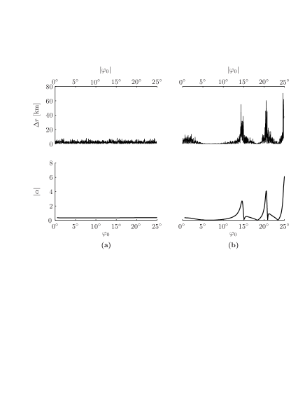
Figure 5: Upper panels: absolute value of the difference between perturbed (rough surface) and unperturbed (flat surface) ray range after 20 surface reflections as a function of initial ray angle at the surface for sound speed profiles PA (a) and PB (b) in Fig. 4. Lower panels: stability parameter as a function of ray angle in each of the two environments.

Figure 4 shows two upward-refracting sound speed profiles. Figure 5 shows $\alpha$ in the same environments and the difference in range, $\Delta r,$ between perturbed (rough surface) and unperturbed (flat surface) rays as a function of launch angle at the surface after making 21 loops, which corresponds to 20 surface reflections. [In this type of environment the definition of $I$ in Eq. (3) is unchanged except that the upper integration limit is $z=0$ for all rays.] Rough surface scattering was treated using a frozen simulated surface gravity wavefield with a $k^{-7/2}$ surface elevation wavenumber spectrum with $0.02$ rad m${}^{-1}\leq k\leq 0.16$ $\mathrm{rad}$ m^-1, $\Delta k=10^{-3}$ rad m${}^{-1},$ and rms slope of $4\times 10^{-3}.$ To treat specular ray reflections from this surface, the surface boundary condition was linearized; the surface elevation was neglected, but the nonzero slope was not approximated.

Figure 5 shows clearly that ray stability, as measured by $\Delta r$, is controlled almost entirely by the background sound speed structure via $\alpha$, rather than details of the rough surface.

IV Shear-induced ray instability

In this section we present additional numerical simulations that give insight into the mechanism by which $\alpha$ influences ray instability. For simplicity we assume deep water conditions here. The arguments presented here make use of the well-known (cf. e.g. Refs. Arnold-89, ; Tabor-89, ) analogy between ray motion, defined by Eqs. (2) and particle motion in an incompressible two-dimensional fluid.

The left panels of Fig. 6 show the range evolution of a segment of a Lagrangian manifold (a smooth curve in phase space) in the unperturbed C89 (top) and cosh (bottom) waveguides. The segment is depicted in black at $r=0$ and in red at $r=1000$ $\unit{km}$ in both waveguides. As a consequence of Liouville’s theorem the segment cannot break or intersect itself but it can increase in complexity as range increases. In the unperturbed case, since the motion is integrable (i.e. each point of the segment preserves its initial $I$), the length of the segment can grow in range, at most, following a power law. The cosh profile has a special property. In that profile the manifold segment just rotates counterclockwise at a constant rate $\omega$. The reason for the difference in behavior is that in the C89 waveguide $\omega$ varies with $I$, whereas in the cosh profile $\omega$ does not vary with $I$. The monotonic decay of $\omega$ as a function of $I$ in the C89 waveguide induces a “shear” in phase space which causes the outermost points of the segment to rotate more slowly than the innermost ones and, hence, causes the segment to spiral. The ray motion in phase space associated with the unperturbed C89 waveguide can thus be regraded as analogous to that of ideal fluid particles passively advected by a stationary planar circular flow with radial shear. In the cosh profile there is no shear. In polar coordinates radial shear can be defined as

$$\rho\frac{\partial}{\partial\rho}\left(\frac{u_{\theta}}{\rho}\right),$$ (10)

where $\rho$ is the radial coordinate and $u_{\theta}$ is the $\theta$-component of the velocity field. (More correctly, this quantity is, apart from a factor of $2$, the $\rho\theta$-component of the strain-rate tensor for planar circular flow; cf. e.g. Ref. Batchelor-64, .) The connection with ray motion in phase space can be accomplished by identifying $I$ with $\rho$ and $\omega I$ with $u_{\theta}$. The replacements $\rho\mapsto I$ and $u_{\theta}\mapsto\omega I$ in Eq. (10) thus give the analogous expression $I\mathrm{d}\omega/\mathrm{d}I$ for the shear in phase space. Notice that this expression is (apart from the $\omega^{-1}$-factor) the stability parameter $\alpha$. We have chosen to include the $\omega^{-1}$-factor in the definition of $\alpha$ because of precedent Zaslavsky-98 and because it is convenient to make $\alpha$ dimensionless.

The right panels of Fig. 6 show the evolution of the Lagrangian manifold segment in the same waveguides as those used to produce the left panels but with a superimposed perturbation induced by internal wave fluctuations. Notice the highly complicated structure of the Lagrangian manifold in the perturbed C89 waveguide as compared to that in the unperturbed one. (Note that the fan of rays used to produce the figure is far too sparse to resolve what should be an unbroken smooth curve which does not intersect itself.) In contrast, observe that in the cosh environment the sound speed perturbation has only a very minor effect on the evolution of the Lagrangian manifold.

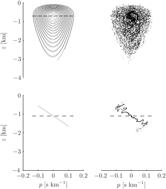
Figure 6: Evolution of a portion of Lagrangian manifold in the C89 (upper panels) and cosh (lower panels) waveguides with (right panels) and without (left panels) internal-wave-induced perturbations. Dashed and solid/dotted curves show the manifold at $r=0$ and $r=1000$ $\unit{km}$, respectively.

Perturbations to steeper rays caused by internal-wave-induced sound speed perturbations in deep ocean, including those in our simulations, are significant only near the ray’s upper turning depth. This observation motivates a simple model that gives insight into the mechanism by which $\alpha$ is linked to ray stability. In the model, each portion of a Lagrangian manifold acquires a sinusoidal “wrinkle” at each upper turning point, but is otherwise unaffected by the sound speed perturbations. The evolution of small segments of a Lagrangian manifold using such a model, in both the C89 and cosh waveguides, is shown in Fig. 7. Notice the rapid growth in complexity of the segment as the range increases in the C89 waveguide. After acquiring a wrinkle, the segment stretches and folds as a result of the radial shear in phase space. As additional wrinkles are acquired this process is repeated successively in range, making the shape of the Lagrangian manifold segment even more complex. In opposition to this situation, observe the simplicity of the segment’s shape in the cosh waveguide as range increases. In this case, after acquiring a wrinkle, the distorted segment rotates counterclockwise, without the additional influence of shear-induced stretching, at a constant frequency $\omega$.

Each time a perturbation is introduced, the action $I$ changes by the amount $\delta I,$ say, which we assume to be of the same order as the perturbation. As a consequence, to lowest-order $R$($=2\pi/\omega$) experiences the change

$$R\mapsto\left(1-\alpha\,\delta I/I\right)R.$$

The perturbation to the range of a ray double loop $R$ depends on both the perturbation and the properties of the background sound speed structure. Under the change $I\mapsto I+\delta I,$ a sufficient condition for $R$ to remain invariant at lowest-order is $\alpha=0.$ This provides an explanation for the remarkable stability of the cosh waveguide. That is, when $\alpha=0$ the ray motion remains periodic at lowest-order—no matter the complexity of the perturbation mounted on the waveguide. To lowest-order, a nonvanishing shear $(\alpha\neq 0)$ appears as a necessary condition to sustain the successive stretching and folding of the Lagrangian manifold after it gets distorted by the perturbation. (Of course, chaotic motion is still possible when $\alpha=0$ provided that the perturbation strength is sufficiently large.) It is thus expected that where $|\alpha|$ is small (resp., large) there will be less (resp., more) sensitivity to initial conditions and, hence, the motion be more regular (resp., chaotic). Support for this conjecture is given in the numerical simulations presented in this paper.

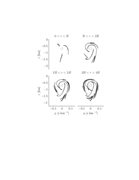
Figure 7: Evolution of a segment of Lagrangian manifold in the C89 (a) and cosh (b) waveguides under the influence of an idealized range-dependent perturbation. The perturbations are is assumed to be in the form of a series of “kicks” that produce a sinusoidal deformation to the Lagrangian manifold at each upper turning depth. The figure shows a portion of Lagrangian manifold, originally located on a torus with frequency $\omega$($=2\pi/R$), immediately after experiencing a kick at range $r=(k-1)R$, $k=1,\cdots,4,$ and before receiving the next one at $r=kR$, as well as at several intermediate stages.

V Summary and discussion

In this paper we have considered ray motion in environments consisting of a range-independent background sound speed profile on which a weak range-dependent perturbation is superimposed. The results presented show that ray stability is strongly influenced by the background sound speed structure; ray instability was shown to increase with increasing magnitude of $\alpha(I)=(I/\omega)\mathrm{d}\omega/\mathrm{d}I,$ where $2\pi/\omega(I)$ is the range of a ray double loop and $I$ is the ray action variable. This conclusion is based largely on numerical simulations, but the simulations were shown to support a simple heuristic argument based on the action–angle form of the ray variational equations. The mechanism by which $\alpha$ controls ray instability was shown to be shear-induced enhancement of perturbations caused by the sound speed perturbation term. The importance of $\alpha$ was illustrated with numerical simulations of ray motion in deep ocean environments including internal-wave-induced scattering, and in upward-refracting environments including rough surface scattering. So far as we are aware, this conclusion is consistent with all of the numerical results presented earlier Duda-Bowlin-94 ; Simmen-Flatte-Yu-Wang-97 ; Smirnov-Virovlyansky-Zaslavsky-01 . Ref. Smirnov-Virovlyansky-Zaslavsky-01, relied heavily on results that follow from a dynamical systems viewpoint.

The connection between our work and results relating to dynamical systems deserves further comment. Recall that the condition $\mathrm{d}\omega/\mathrm{d}I\neq 0$ (the nondegeneracy condition) must be satisfied for the KAM theorem to apply, and that this result guarantees that some rays are nonchaotic provided the strength of the range-dependent perturbation is sufficiently weak. This theorem might seem to conflict with our assertion that ray instability increases with increasing $\left|\alpha\right|.$ This apparent conflict can be resolved by interpreting our statement as a statement of what happens for most rays. That is, for most rays stability exponents (finite range estimates of Lyapunov exponents) increase as $\left|\alpha\right|$ increases. This does not rule out the possibility that for a fixed $\mathrm{d}\omega/\mathrm{d}I\neq 0$ some rays will be nonchaotic.

A seemingly more troublesome conflict between our simulations and KAM theory follows from the result, noted earlier, that each isolated resonance has a width proportional to $|\mathrm{d}\omega/\mathrm{d}I|^{-1/2}$. Doesn’t this imply that rays should become increasingly chaotic as $|\mathrm{d}\omega/\mathrm{d}I|$ decreases? The answer, we believe, is no. To understand why, consider rays in a band $I_{0}\leq I\leq I_{1}$ over which $\mathrm{d}\omega/\mathrm{d}I$ is approximately constant, $\mathrm{d}\omega/\mathrm{d}I=(\omega_{1}-\omega_{0})/(I_{1}-I_{0})$. Within this band resonances are excited at selected values of $\omega$. The number of resonances excited is approximately proportional to $|\omega_{1}-\omega_{0}|$, which, in turn, is proportional to $|\mathrm{d}\omega/\mathrm{d}I|$. The “degree of chaos” should be proportional to the product of the number of resonances excited and the width of individual resonances. This product scales like $|\mathrm{d}\omega/\mathrm{d}I|^{1/2}$; this suggests that rays should become increasingly chaotic as $|\mathrm{d}\omega/\mathrm{d}I|$ increases, consistent with our simulations. Neither the KAM theorem nor the resonance width estimate estimate applies in the limit $\mathrm{d}\omega/\mathrm{d}I=0$. Behavior in that limit is likely problem-dependent (e.g. Refs. Chernikov-et-al-87, ; Chernikov-Sagdeev-Zaslavsky-88, ). Our simulations—which are probably representative of problems characterized by an inhomogeneous background and a weak perturbation with a broad spectrum—suggest that ray motion in this limit is very stable.

In this paper we have addressed the issue of ray stability in physical space or phase space; we have not addressed the related problem of travel time stability. The latter problem is more difficult inasmuch as that problem involves, in addition to the (one-way) ray equations (2), a third equation $\mathrm{d}T/\mathrm{d}r=L$ and imposition of an eigenray constraint. Here, $L=p\mathrm{d}z/\mathrm{d}r-h(p,z;r)$ using standard variables, or $L=I\mathrm{d}\vartheta/\mathrm{d}r-\bar{h}(I,\vartheta;r)$ using action–angle variables. We have seen some numerical evidence that ray instability in phase space is linked to large time spreads, but this connection is currently not fully understood.

An advantage of our use of the action–angle formalism is that essentially the same results apply if the assumption of a background range-independent sound speed profile, i.e. $C=C(z),$ is relaxed to allow for a slowly-varying (in range) background sound speed structure, i.e. $C=C(z;\varepsilon r).$ (Here, $\varepsilon$ scales like the ratio of a typical correlation length of the range-dependence to a typical ray double loop range.) In the latter case the action is not an exact ray invariant but it is an adiabatic invariant, i.e. $\mathrm{d}I/\mathrm{d}r=O(\varepsilon^{2}).$ Thus, correct to $O(\varepsilon)$ the latter problem can be treated as being identical to the former one. Consequently, the problem that we have treated here also applies to slowly-varying background environments.

APPENDIX: STABILITY EXPONENTS

Liouville’s theorem (cf. e.g. Refs. Arnold-89, ; Tabor-89, ) guarantees that areas in the present two-dimensional phase space are preserved, leading to $\det\mathsf{Q}=1$ as a corollary. Consequently, $2\nu_{\pm}^{\mathsf{Q}}=\mathop{\mathrm{t}race}\mathsf{Q}\pm\sqrt{\mathop{\mathrm{t}race}^{2}\mathsf{Q}-1}$. (It can be shown that $\nu_{\pm}^{\mathsf{Q}}\sim\mathop{\mathrm{t}race}^{\pm 1}\mathsf{Q}$ as $r\rightarrow\infty$; accordingly, Eq. (8) can be replaced by the equivalent expression $\nu=$ $\lim\nolimits_{r\rightarrow\infty}$ $r^{-1}\ln\left|\mathop{\mathrm{t}race}\mathsf{Q}\right|$ as in Ref. 20.) The condition $\det\mathsf{Q}=1$, however, is difficult to fulfill in highly chaotic flows due to the limitation of machine numerical precision. More precisely, an initial area in phase space tends to align along the one-dimensional perturbation subspace spanned by the eigenvector of $\mathsf{Q}$ associated with the largest Lyapunov exponent, making the elements of $\mathsf{Q}$ ill-conditioned. This implies that neither $\det\mathsf{Q}$ nor $\mathop{\mathrm{t}race}\mathsf{Q}$—and, hence, neither $\nu^{\mathsf{Q}}$ nor $\nu_{\infty}$—can be computed reliably at long range. The common approach to overcome this problem involves successive normalizations of the elements of $\mathsf{Q},$ while integrating simultaneously (2) and (7), after a fixed number of range steps Parker-Chua-89 . An alternative strategy, which does not involve normalizations, has been taken here.

Let $\mathsf{A}(r)$ be the bounded-element matrix such that

$$\mathsf{Q}=\mathsf{A}\,\mathrm{e}^{\lambda r},$$ (11)

which implies

$$\nu^{\mathsf{Q}}=\nu^{\mathsf{A}}\mathrm{e}^{\lambda r}.$$

Here, $\lambda$ is a guessed value of $\nu_{\infty}.$ The reason for introducing the decomposition (11) is that if $\lambda$ is close to $\nu_{\infty},$ the matrix $\mathsf{A}$ will remain well conditioned at ranges long past those at which $\mathsf{Q}$ becomes poorly conditioned. This leads, in turn, to significantly improved numerical stability. Eq. (7) leads to the modified variational equations

$$\frac{\mathrm{d}\mathsf{A}}{\mathrm{d}r}=\left(\mathsf{J}-\lambda\mathsf{I}\right)\mathsf{A},\quad\mathsf{A}(0)=\mathsf{I}.$$ (12)

Notice that $\det\mathsf{Q}=\det\mathsf{A\,}\mathrm{\exp}\lambda r=1$ and, hence, $\det\mathsf{A}\sim 0\;$as $r\rightarrow\infty.$ Eq. (12) has been integrated in this paper after choosing $\lambda$, in order to compute a finite range estimate of $\nu_{\infty}$, which we call a stability exponent and denote by $\nu.$

References

- (1) T. F. Duda, S. M. Flatté, J. A. Colosi, B. D. Cornuelle, J. A. Hildebrand, W. S. Hodgkiss, P. F. Worcester, B. M. Howe, J. A. Mercer, and R. C. Spindel, “Measured Wavefront Fluctuations in 1000 Km Pulse Propagation in the Pacific Ocean,” J. Acoust. Soc. Am. 92, 939–955 (1992).
- (2) P. F. Worcester, B. D. Cornuelle, M. A. Dzieciuch, W. H. Munk, J. A. Colosi, B. M. Howe, J. A. Mercer, A. B. Baggeroer, and K. Metzger, “A Test of Basin-Scale Acoustic Thermometry Using a Large-Aperture Vertical Array at 3250-Km Range in the Eastern North Pacific Ocean,” J. Acoust. Soc. Am. 105, 3,185–3,201 (1999).
- (3) J. A. Colosi et al., “Comparison of Measured and Predicted Acoustic Fluctuations for a 3250-Km Propagation Experiment in the Eastern North Pacific Ocean,” J. Acoust. Soc. Am. 105, 3,202–3,218 (1999).
- (4) T. F. Duda and J. B. Bowlin, “Ray-Acoustic Caustic Formation and Timing Effects from Ocean Sound-Speed Relative Curvature,” J. Acoust. Soc. Am. 96, 1,033–1,046 (1994).
- (5) J. Simmen, S. M. Flatté, and G. Yu-Wang, “Wavefront Folding, Chaos and Diffraction for Sound Propagation Through Ocean Internal Waves,” J. Acoust. Soc. Am. 102, 239–255 (1997).
- (6) I. P. Smirnov, A. L. Virovlyansky, and G. M. Zaslavsky, “Theory and Application of Ray Chaos to Underwater Acoustics,” Phys. Rev. E 64, 036221, 1–20 (2001).
- (7) M. G. Brown, J. A. Colosi, S. Tomsovic, A. L. Virovlyansky, M. Wolfson, and G. M. Zaslavsky, “Ray Dynamics in Ocean Acoustics,” J. Acoust. Soc. Am. (2003), in press.
- (8) V. I. Arnold, Mathematical Methods of Classical Mechanics (Springer, 1989).
- (9) M. Tabor, Chaos and Integrability in Nonlinear Dynamics (John Wiley and Sons, 1989).
- (10) G. M. Zaslavsky, Physics of Chaos in Hamiltonian Systems (Imperial College, 1998).
- (11) B. V. Chirikov, “A Universal Instability of Many-Dimensional Oscillator Systems,” Phys. Rep. 52, 265–379 (1979).
- (12) M. G. Brown, “Phase Space Structure and Fractal Trajectories in One-and-a-Half Degree of Freedom Hamiltonian Systems Whose Time Dependence is Quasiperiodic,” Nonlinear Processes in Geophys. 5, 69–74 (1998).
- (13) W. H. Munk, “Sound Channel in an Exponentially Stratified Ocean with Application to SOFAR,” J. Acoust. Soc. Am. 55, 220–226 (1974).
- (14) M. A. Wolfson and J. L. Spiesberger, “Full Wave Simulation of the Forward Scattering of Sound in a Structured Ocean: A Comparison with Observations,” J. Acoust. Soc. Am. 106, 1293–1306 (1999).
- (15) F. J. Beron-Vera, M. G. Brown, J. A. Colosi, S. Tomsovic, A. L. Virovlyansky, M. A. Wolfson, and G. M. Zaslavsky, “Ray Dynamics in a Long-Range Acoustic Propagation Experiment,” J. Acoust. Soc. Am. (2002), submitted.
- (16) W. H. Munk, “Internal Waves and Small Scale Processes,” In Evolution of Physical Oceanography, B. Warren and C. Wunsch, eds., pp. 264–291 (MIT, 1981).
- (17) J. A. Colosi and M. G. Brown, “Efficient Numerical Simulation of Stochastic Internal-Wave-Induced Sound Speed Perturbation Fields,” J. Acoust. Soc. Am. 103, 2,232–2,235 (1998).
- (18) G. K. Batchelor, An Introduction to Fluid Dynamics (Cambridge University, 1964).
- (19) A. A. Chernikov, M. Y. Natenzon, B. A. Petrovichev, R. Z. Sagdeev, and G. M. Zaslavsky, “Some Peculiarities of Stochastic Layer and Stochastic Web Formation,” Phys. Let. A 122, 39–46 (1987).
- (20) A. Chernikov, R. Sagdeev, and G. Zaslavsky, “Chaos: How Regular Can It Be?,” Physics Today 41, 27–35 (1988).
- (21) M. A. Wolfson and S. Tomsovic, “On the Stability of Long-Range Sound Propagation Through a Structured Ocean,” J. Acoust. Soc. Am. 109, 2,693–2,703 (2001).
- (22) T. S. Parker and L. O. Chua, Practical Numerical Algorithms for Chaotic Systems (Springer, 1989).