Fractal analysis on a closed classical hard-wall billiard using a simplified box-counting algorithm

Abstract

We perform fractal analysis on a closed classical hard-wall billiard, the circular billiard with a straight cut, assuming there are two openings on the boundary. We use a two-dimensional set of initial conditions that produce all possible trajectories of a particle injected from one opening, and numerically compute the fractal dimension of singular points of a function that maps an initial condition to the number of collisions with the wall before the exit. We introduce a simplified box-counting algorithm, which uses points from a rectangular grid inside the two-dimensional set of the initial conditions, to simplify the calculation, and observe the classical chaotic properties while varying the parameters of the billiard.

Chaotic systems have recently attracted many researchers from various fields, partly because the fast development of computer hardwares has enabled us to solve equations almost insolvable in the pastOtt (1993); Reichl (1992). For physicists, the two-dimensional (2D) billiard system has been a popular subject for studying the dynamics of the Hamiltonian chaotic systems. Classically, the dynamics of the 2D billiard system shows three distinct types of behaviors. The system is either integrable (regular behavior) or non-integrable (either soft chaos, characterized by mixed phase spaces that have both regular and chaotic regions, or hard chaos, characterized by ergodicity and mixing)Gutzwiller (1990).

Here we use a closed 2D hard-wall billiard with two openings on the boundary, and perform fractal analysis using the classical dynamics while varying the shape of the bliiard and the size of the openings. To calculate the fractal dimension, we use a set of initial conditions that will produce trajectories of a particle injected from one opening, and calculate certain values for each trajectory, such as the exit opening (an opening from which the particle exits), the number of collisions with the wall before the exit, the dwell time, and so on. When the system is chaotic, singular points of this kind of response functions form a fractal setEckhardt (1987); Bleher et al. (1988); Ott and Tél (1993). In this Letter, we will calculate the fractal dimension of these singular points of the function that maps an initial condition to the number of collisions, by introducing a simplified box-counting algorithm.

The billiard we have chosen is the circular billiard with a straight cut, or the “cut-circle” billiard (see Fig. 1).

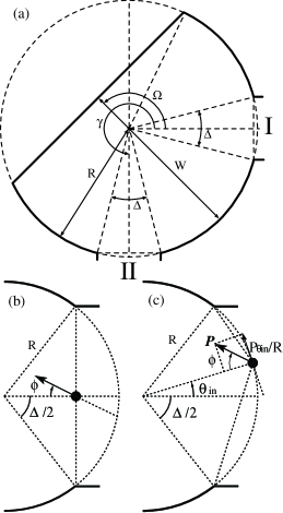
Figure 1: (a) Geometry of the cut-circle billiard. There are two openings, I and II, and a straight cut. The size of the cut is given by the width $W$ (here we use $w\equiv W/R$ as the relative size of the cut), and the size of two openings is $\Delta$. The positions of the cut and the opening II, $\Omega$ and $\gamma$, are measured from the position of the opening I. (b) When a particle is injected from the central point of the opening I with an angle $\phi$, the set of possible initial conditions is one dimensional $(-\pi/2<\phi<\pi/2)$. (c) To fully represent all significant initial conditions, a particle is injected from a point on the circular boundary of the opening I with the angular momentum $P_{\theta\rm in}$. This set, whose element is represented by a pair of values, $(\theta_{\rm in},P_{\theta\rm in})$, is a closed two-dimensional subspace of the four-dimensional phase space.

There are five parameters: (1) the width $W$ measured in the direction perpendicular to the cut, (2) the radius $R$, (3) the angular width $\Delta$ of the openings, which represents the opening size, (4) the orientation angle ${\Omega}$ of the cut relative to the first opening, and (5) the position of the second opening relative to the first opening as measured by the angle $\gamma$. We scale the width $W$ by $R$, so $w\equiv W/R$, thereby reducing the number of independent parameters to four: $w$, $\Delta$, $\Omega$, and $\gamma$. For all subsequent discussions, we set $\Omega=135^{\circ}$ and $\gamma=270^{\circ}$. For the closed cut-circle billiard (when $\Delta=0$), it has been proved in Ref. Bunimovich, 1979 that the phase space is mixed (soft chaos) when $0<w<1$, and that the phase space is fully chaotic (hard chaos) when $1<w<2$. And it is integrable when $w=1$ and 2. Consequently this billiard has a single shape parameter $w$ that makes the billiard exhibit all three types of chaotic behaviors.

In Ref. Ree, 2002, a one-dimensional (1D) set of initial conditions of the cut-circle billiard was used to calculate fractal dimensions while varying the opening size $\Delta$ and the shape parameter $w$ [see Fig. 1(b)]. The particle is injected with an incident angle $\phi$ ($-\pi/2<\phi<\pi/2$). In Ref. Legrand and Sornette, 1990, authors used a 1D set of initial conditions for the stadium, and calculated the recurrence time for each trajectory to obtain the fractal dimension. These 1D sets, however, are subsets of the set of all significant initial conditions that represent all possible trajectories; in our billiard, a 2D subspace in the four-dimensional (4D) phase space is a minimal set that will produce all possible trajectories originating from one opening [see Fig. 1(c)]. (A 2D set of initial conditions were also used in Ref. Bleher et al., 1988 for the Sinai billiard.) There are two reasons that make this reduction possible. First, the value of the energy does not change the trajectory of the particle. This is due to the flat potential inside the billiard with infinitely hard boundaries. Second, the distance from the center of the billiard to the initial location of the particle can be fixed at $R$.

With these two kinds of sets, we numerically find a function that maps an initial condition to the number of collisions before the exit. (In numerical computations, all possible initial conditions cannot be used; only a finite and discrete subset can be considered.) In Fig. 2, we show how the number of collisions changes for these sets of initial conditions when $w=1.5$ and $\Delta=60^{\circ}$.

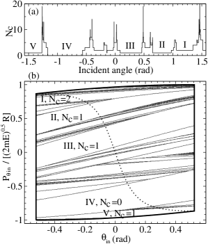
Figure 2: Calculations of the number of collisions when $\Omega=135^{\circ}$, $\gamma=270^{\circ}$, $w=1.5$, and $\Delta=60^{\circ}$. (a) Graph of the incident angle $\phi$ vs the number of collisions $N_{C}$ when the particle is injected as in Fig. 1(b). (b) When the particle is injected as in Fig. 1(c), all significant initial conditions lie inside the closed two-dimensional space bounded by the bold line in the graph. In the graph, only singular points are shown. The dotted line represents the one-dimensional subset of initial conditions used in (a). Five geometrical channels with low $N_{C}$’s are also shown.

In Fig. 2(a), the graph of $\phi$ vs the number of collisions is shown when the 1D subset of initial conditions as in Fig. 1(b) is used (see Ref. Ree, 2002 for more results). In Fig. 2(b), the graph shows the full 2D set of initial conditions, $(\theta_{\rm in},P_{\theta\rm in})$, bounded by two equations,

$$-\frac{\Delta}{2}\leq\theta{\rm in}\leq\frac{\Delta}{2},$$ (1)

$$-\cos\left(\frac{\Delta}{4}+\frac{\theta_{\rm in}}{2}\right)\leq\frac{P_{\theta\rm in}}{\sqrt{2mE}R}\leq\cos\left(\frac{\Delta}{4}-\frac{\theta_{\rm in}}{2}\right),$$ (2)

which are represented by the bold line. Instead of the number of collisions, the graph shows singular points that constitute singular boundaries at which the number of collisions changes. We can observe that singular points have infinitely fine structures. The number of collisions are shown only for five geometrical channelsRoukes and Alerhand (1990); Luna-Acosta et al. (1996) in this example. The dotted line is the 1D subset used in Fig. 2(a).

Now we calculate the fractal dimension $d_{f}$ of a set of singular points in this 2D set using a simplified box-counting algorithm. As a generalization of the box-counting algorithm used in Ref. Ree, 2002 for the 1D set, we use a uniform 2D rectangular grid. Then there are uniform rectangular boxes, and each of them is represented by four points on the grid. For all of these uniformly distributed grid points inside the 2D set, we numerically find the number of collisions before the exit, and for each box, we compare the number of collisions at four corners. With an assumption that a box does not contain a singular point when four values are all equal, we can count the number of boxes containing singularities out of all boxes inside the 2D set. The number of all boxes inside the set is $N_{P}$, and the number of boxes that contain any singular point, based on the above assumption, is $N_{S}$. Then the fractal dimension $d_{f}$ is defined by

$$d_{f}\equiv\lim_{N_{P}\rightarrow\infty}\frac{\log_{10}{N_{S}}}{\log_{10}{N_{P}}^{1/2}},$$ (3)

which is the slope of the graph of $0.5\log_{10}{N_{P}}$ vs $\log_{10}{N_{S}}$. In numerical calculations, we find $N_{S}$ for several $N_{P}$ values, and then use the ordinary least-square fit to find the slope using the points in the graph.

In Fig. 3(a), the log-log graph is shown for several $\Delta$ values when $w=1.5$. (For all calculations, $N_{P}$ up to $10^{8}$ will be used.)

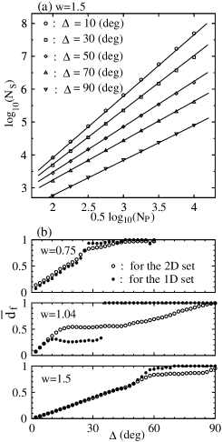
Figure 3: (a) When $w=1.5$, the number of boxes containing the singular points, $N_{S}$, is counted as the number of boxes, $N_{P}$, increases, for five different $\Delta$ values. Then $d_{f}$ can be found from the slopes of these log-log graphs. (b) Graphs of $\bar{d_{f}}$ vs the opening size $\Delta$ for $w=0.75$, $1.04$, and $1.5$. Here we compare the values of $\bar{d_{f}}$ for the 2D set ($\circ$) and for the 1D set ($*$).

Unlike the calculations using the 1D set, $d_{f}$ will be in the range of $1\leq d_{f}\leq 2$. We can define $\bar{d_{f}}$, which better represents the fractality,

$$\bar{d_{f}}\equiv\left\{\begin{array}[]{rl}2-d_{f}{}&\mbox{(for the 2D set)}\\ 1-d_{f}{}&\mbox{(for the 1D set)}\end{array}\right..$$ (4)

In Fig. 3(b), $\bar{d_{f}}$’s both for the 2D set and for the 1D set are compared for three different $w$ values while varying $\Delta$. Like the curves for the 1D set, not all curves monotonically increase as $\Delta$ increases, even though it is not as significant. The reason for this phenomenon is that there are more possible trajectories when the opening gets bigger, and it also explains why curves don’t match very well for large $\Delta$. We also observe that the cases with hard chaos ($w=1.04$, and 1.5) do not behave predictably for large $\Delta$, which will be more clearly seen in the following graph. When the original shape is changed sufficiently by the presence of the openings, the ergodicity of the billiard is no longer an important factor; the relative locations of the openings start to have more effect on the fractal dimension as in the cases of soft chaos.

In Fig. 4, we calculate $\bar{d_{f}}$ as the width $w$ varies from 0.5 to 2 with a step size of 0.02 for seven opening sizes ($\Delta=1^{\circ}$, $\Delta=5^{\circ}$, $\Delta=10^{\circ}$, $\Delta=20^{\circ}$, $\Delta=30^{\circ}$, $\Delta=40^{\circ}$, and $\Delta=50^{\circ}$), using the 2D set.

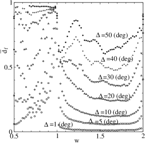
Figure 4: Graphs of $w$ vs $\bar{d_{f}}$ for seven different opening sizes: $\Delta=1^{\circ}$ ($\circ$), $\Delta=5^{\circ}$ ($\Box$), $\Delta=10^{\circ}$ ($\Diamond$), $\Delta=20^{\circ}$ ($\bigtriangleup$), $\Delta=30^{\circ}$ ($\bigtriangledown$), $\Delta=40^{\circ}$ ($+$), and $\Delta=50^{\circ}$ ($*$), for the 2D set. When $\Delta$ is small enough ($\Delta\leq 20^{\circ}$ in the graph), the behavior of the graph is clearly distinct for two regions: hard chaos ($1<w<2$) and soft chaos ($0<w<1$). But for larger $\Delta$, the distinction between two regions starts to disappear.

We can compare graphs in two different regions (found in the closed cut-circle billiard): $0<w<1$ (soft chaos) and $1<w<2$ (hard chaos). We observed similar behaviors seen in results for the 1D set in Ref. Ree, 2002. However $\bar{d_{f}}$ does not reach one ($\bar{d_{f}}=1$ represents non-chaos), even when the billiard is integrable ($w=1$ or 2), and this is due to the fine structure near trajectories bouncing very close to the circular boundary. When the opening size $\Delta$ is not big (see graphs for $\Delta=5^{\circ}$, $\Delta=10^{\circ}$, and $\Delta=20^{\circ}$), we observe that the behavior in two regions is clearly distinct. In the region $0<w<1$, there are fluctuations, which comes from the mixed phase space structures of the billiard, and in the region $1<w<2$, graphs are smooth because the phase spaces of the billiard have no structure due to ergodicity. On the other hand, when the opening size gets bigger (see graphs for $\Delta=30^{\circ}$, $\Delta=40^{\circ}$, and $\Delta=50^{\circ}$), the distinction between two regions, observed in cases with smaller openings, disappears. There are fluctuations in both regions.

In this Letter, we calculated the fractal dimension for the cut-circle billiard with two openings by introducing the simplified box-counting algorithm for the 2D set of initial conditions. The simplified box-counting algorithm introduced here is possible because the function used to find singularities is constant except singular points (i. e., the function is constant with different values in all regions surrounded by singular boundaries). With this method, some boxes containing singular points will be missed, but the number of missed boxes is negligible when we calculate the fractal dimension with big enough $N_{P}$ values. Results for the 2D set were close to those for the 1D set only when $\Delta$ is small enough; hence using the 1D set in fractal analysis does not fully represent the chaoticity of the billiard for most cases. In conclusion, this kind of fractal analyses gives us one of the fundamental measures of the chaoticity of classical billiard systems, and finding the relations with the quantum and semiclassical dynamics of the same kind of billiards will be one of the interesting future works.