Synchronizing to Periodicity:
The Transient Information and Synchronization Time of Periodic Sequences

Abstract

We analyze how difficult it is to synchronize to a periodic sequence whose structure is known, when an observer is initially unaware of the sequence’s phase. We examine the transient information ${\bf T}$, a recently introduced information-theoretic quantity that measures the uncertainty an observer experiences while synchronizing to a sequence. We also consider the synchronization time ${\tau}$, which is the average number of measurements required to infer the phase of a periodic signal. We calculate ${\bf T}$ and ${\tau}$ for all periodic sequences up to and including period $23$. We show which sequences of a given period have the maximum and minimum possible ${\bf T}$ and ${\tau}$ values, develop analytic expressions for the extreme values, and show that in these cases the transient information is the product of the total phase information and the synchronization time. Despite the latter result, our analyses demonstrate that the transient information and synchronization time capture different and complementary structural properties of individual periodic sequences — properties, moreover, that are distinct from source entropy rate and mutual information measures, such as the excess entropy.

PACS: 02.50.Ey 02.50.Ga 05.45.-a 05.45.Tp 89.75.Kd;

Santa Fe Institute Working Paper 02-08-043

I Introduction

Imagine you are about to begin observing a sequence of events. You know the sequence is periodic; you even know the particular pattern that will repeat. However, you do not know what phase the sequence is in. How many observations, on average, would you have to make before you know with certainty the sequence’s phase? And, as you obtain this certainty, how uncertain are you about the phase? Will the answers to these questions be the same for all sequences of a given period or are there differences between such sequences? What structural properties of a sequence determine the difficulty of synchronization? Here, we answer these questions.

A natural place to begin is with information theory, since it has long been used to analyze the statistical properties of sequences that arise in a variety of settings, including dynamical systems, time-series analysis, statistical mechanics, signal processing, and cryptography [1, 2]. One of the central quantities in these analyses is the entropy rate $h_{\mu}$, the long-time measure of unpredictability of sequences produced by an information source. Although useful and important for quantifying randomness, $h_{\mu}$ does not capture a sequence’s structural properties: its correlation, memory, or statistical complexity. Fortunately, today there are scores of measures of these latter properties. For example, on the information theoretic side, an oft-used measure of memory is the excess entropy ${\bf E}$ — the time-averaged, “all-point” mutual information between a sequence’s past and future [3, 4, 5, 6, 7].

For any sequence of period $P$, it is well known that the entropy rate $h_{\mu}$ vanishes and the excess entropy ${\bf E}=\log_{2}P$, since a periodic sequence is asymptotically predictable and since $\log_{2}P$ bits of information are needed to store in which of the $P$ possible phases a symbol in the sequence is. Thus, all periodic sequences of the same period have the same entropy rate and excess entropy, and so these quantities are unable to capture structural differences between distinct sequences of the same period. In particular, $h_{\mu}$ and ${\bf E}$ cannot help answer the questions posed above.

We turn instead to a recently introduced measure, the transient information ${\bf T}$ [5, 8], which captures information-theoretic differences between sequences of a given period. We will also make use of the synchronization time ${\tau}$, defined as the average number of observations needed to synchronize to a periodic information source. We shall see that there are indeed significant differences in the synchronization properties of periodic sequences. Furthermore, while ${\bf T}$ and $\tau$ are related for extreme cases — minimum and maximum ${\bf T}$ and $\tau$ sequences — there is a wide range of ${\bf T}$ and $\tau$ values for periodic sequences of the same period.

In the following section we review information sources, entropy rate, and excess entropy. In Sec. III we define ${\bf T}$ and ${\tau}$ more carefully. After a brief discussion of combinatorics and symmetry types of periodic sequences in Sec. IV, in Sec. V we discuss methods used to calculate ${\bf T}$ and ${\tau}$. In Sec. VI we present the results of exhaustively calculating ${\bf T}$ and ${\tau}$ up to period $23$. In Secs. VII and VIII, we investigate these results, developing analytic expressions for the minimum and maximum ${\bf T}$ and ${\tau}$ values of a given period, exploring relationships and bounds between the two synchronization measures. Finally, in Sec. IX we summarize and interpret the results, pointing out several applications to coordination in multiagent systems.

II Entropy Rate and Excess Entropy

A Information Sources

We shall be concerned with a one-dimensional infinite sequence of variables:

$$\stackrel{{\scriptstyle\leftrightarrow}}{{S}}\,\equiv\,\ldots S_{-2}S_{-1}S_{0}S_{1}\ldots\;.$$ (1)

Here, the $S_{t}$’s are random variables that range over a finite set ${\cal A}$ of alphabet symbols. In general, ${\cal A}=\{0,1,\ldots,k-1\}$, although in the following, we will restrict ourselves to binary sequences. We denote a block or word of $L$ consecutive variables by $S^{L}\equiv S_{1}\ldots S_{L}$. We follow the convention that a capital letter refers to a random variable, while a lowercase letter denotes a particular value of that variable. Thus, $s^{L}=s_{0}s_{1}\cdots s_{L-1}$, denotes a particular symbol block of length $L$.

We assume that the underlying information source is described by a shift-invariant measure $\mu$ on infinite sequences $\cdots s_{-2}s_{-1}s_{0}s_{1}s_{2}\cdots;s_{t}\in\cal A$ [9]. The measure $\mu$ induces a family of distributions, $\{{\rm Pr}(s_{t+1},\ldots,s_{t+L}):s_{t}\in\cal A\}$, where ${\rm Pr}(s_{t})$ denotes the probability that at time $t$ the random variable $S_{t}$ takes on the particular value $s_{t}\in\cal A$ and ${\rm Pr}(s_{t+1},\ldots,s_{t+L})$ denotes the joint probability over blocks of $L$ consecutive symbols. We assume that the source is stationary; ${\rm Pr}(s_{t+1},\ldots,s_{t+L})={\rm Pr}(s_{1},\ldots,s_{L})$.

We are interested in periodic sequences; a sequence is periodic of period $P$ if $s_{i}=s_{i+P}$ for all $i$. The prime period of the sequence is the smallest such $P$. We can specify a periodic sequence by giving the smallest word — the prime word — that is exactly repeated. The prime word is aperiodic, necessarily. For example, $\ldots 1100110011001100\ldots$ is period $8$ (and period $16$ and so on), but has prime word $1100$ and prime period $4$.

B Entropy Growth and Entropy Rate

Here, we give a brief review of the information-theoretic description of sequences, concentrating on those that are periodic. For more detail about information-theoretic measures of uncertainty and structure in the context of general one-dimensional random sequences, see, e.g., Refs. [5, 10, 11] and references therein.

The total Shannon entropy of length-$L$ blocks is defined by:

$$H(L)\,\equiv\,-\sum_{s^{L}\in{\cal A}^{L}}{\rm Pr}(s^{L}){\rm log}_{2}{\rm Pr}(s^{L})\;,$$ (2)

where $L>0$. The sum is understood to run over all possible blocks of $L$ consecutive symbols. The units of $H(L)$ are bits. The entropy $H(L)$ measures the average uncertainty in identifying one sequence in the set of length-$L$ sequences. Equivalently, $H(L)$ tells us how many yes-no questions, on average, are needed to determine the value of $S^{L}$. Another way to state this is that $H(L)$ sets a lower bound on the size of the code, measured in bits, needed to encode successive outcomes of the random variable $S^{L}$. For more on this coding interpretation of the Shannon entropy, see, e.g., Ref. [2].

The general behavior of $H(L)$ as a function of $L$ for periodic information sources is shown schematically in Fig. 1. Note that we define $H(0)\equiv 0$.

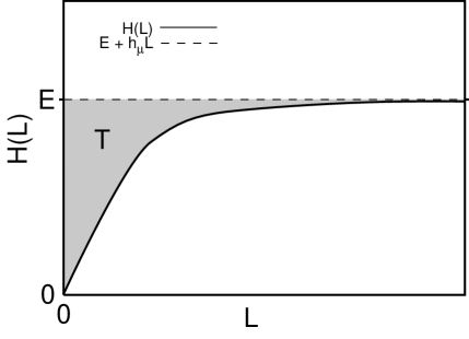
FIG. 1.: Total Shannon entropy growth: A schematic plot of $H(L)$ versus $L$. The entropy $H(L)$ of $L$-blocks increases monotonically and approaches the asymptote ${\bf E}+h_{\mu}L$, where ${\bf E}$ is the excess entropy and $h_{\mu}$ is the source entropy rate. The shaded area is the transient information ${\bf T}$.

The entropy rate $h_{\mu}$ is the rate of increase with respect to $L$ of the total Shannon entropy in the large-$L$ limit:

$$h_{\mu}\equiv\lim_{L\rightarrow\infty}\frac{H(L)}{L}\;,$$ (3)

where $\mu$ denotes the measure over infinite sequences that induces the $L$-block joint distribution ${\rm Pr}(S^{L})$; the units are bits per symbol. One can also define a finite-$L$ approximation to $h_{\mu}$,

$$h_{\mu}(L)\, = \,H(L)-H(L\!-\!1)\;,$$ (4)

$$= \,H[S_{L}|S_{L-1}S_{L-2}\ldots S_{0}]\;,$$ (5)

where $H[X|Y]$ is the entropy of the random variable $X$ conditioned on the random variable $Y$: $H[X|Y]\,\equiv\,-\sum_{x,y}{\rm Pr}(x,y)\log_{2}{\rm Pr(x|y)}$. One can then show [2] that

$$h_{\mu}=\lim_{L\rightarrow\infty}h_{\mu}(L)\;.$$ (6)

Note that Eq. (4) shows that $h_{\mu}(L)$ may be viewed as the slope of $H(L)$. For more on this point of view, see Ref. [5].

Eq. (6) gives us another interpretation of $h_{\mu}$. The entropy rate quantifies the irreducible randomness or unpredictability of the sequences; $h_{\mu}$ measures the randomness that persists even after the statistics of longer and longer blocks are taken into account. Since all periodic sequences are, ultimately, predictable, the entropy rate for all periodic sequences is $h_{\mu}=0$. For a period-$P$ sequence $h_{\mu}(P)=0$ and $h_{\mu}(L)\geq 0$, for $L=1,2,\ldots,P\!-\!1$. This is illustrated in Fig. 2 for three different period-$8$ sequences; when the slope of $H(L)$ vanishes, $h_{\mu}(L)=0$.

FIG. 2.: Shannon entropy growth curves $H(L)$ for three different period-$8$ sequences: $00010111$, $00010101$, and $00000001$.

C Excess Entropy: Apparent Memory

The entropy rate measures the randomness of sequences. A complementary quantity is the excess entropy ${\bf E}$, which measures the deviations of finite-$L$ estimates of $h_{\mu}$ from its asymptotic value:

$${\bf E}\,\equiv\,\sum_{L=1}^{\infty}[h_{\mu}(L)-h_{\mu}]\;,$$ (7)

The units of ${\bf E}$ are bits. Using this definition, one can show that the excess entropy is the subextensive part of $H(L)$ (see, e.g., [4, 5, 11, 12, 13, 7]); that is,

$${\bf E}=\lim_{L\rightarrow\infty}[H(L)-h_{\mu}L]\;.$$ (8)

This establishes a geometric interpretation for ${\bf E}$, as shown in Fig. 1; it is the $y$-intercept of the line to which $H(L)$ asymptotes. That is, when ${\bf E}$ is finite, $H(L)$ asymptotes to ${\bf E}+h_{\mu}L$.

Another way to understand excess entropy is through its expression as a mutual information: the mutual information between the past and future semi-infinite halves of the chain of random variables:

$${\bf E}\,=\,\lim_{L\rightarrow\infty}I[S_{-L+1},S_{-L+2},\cdots S_{0};S_{1}S_{2}\cdots S_{L}]\;,$$ (9)

when the limit exists [5, 7]. Eq. (9) says that ${\bf E}$ measures the amount of historical information stored in the present that is communicated to the future.

Our focus here is on periodic sequences, for which it is easy to show from one or another of the above definitions that

$${\bf E}={\rm log}_{2}P~{}.$$ (10)

That is, the excess entropy is the total phase information stored in the periodic source. As noted above, the entropy of a random variable gives the average number of yes-no questions (i.e., bits), needed to determine the outcome of the variable. Since the observer starts out equally ignorant of the initial phase, it follows that ${\bf E}$ is a lower bound on the amount of information (in bits) an observer must extract in order to know in which phase the source is — that is, in order for it to be synchronized to the source.

The entropy growth curves $H(L)$ for three different period-$8$ sequences are shown in Fig. 2. Note that all curves asymptote to the same line, ${{\bf E}}+h_{\mu}L$. Since $h_{\mu}=0$ (periodic sequences) and ${{\bf E}}=\log_{2}P=\log_{2}8=3$, the $H(L)$ curves asymptote to the horizontal line $H(L)=3$ bits, when $L\geq 8$.

Despite the fact that these three period-$8$ sequences have the same $h_{\mu}$ and ${{\bf E}}$, Fig. 2 shows that their entropy growth curves $H(L)$ are not the same; for example, they reach the linear asymptote at different $L$’s. Do all period-$8$ curves have different $H(L)$ behaviors? And do these different $H(L)$ behaviors matter, or do $h_{\mu}$ and ${\bf E}$ suffice to characterize periodic sequences?

III Measures of Synchronization

A Transient Information

To address these questions, we consider the transient information ${\bf T}$, which was introduced by us in Ref. [5] and is defined by summing the deviations of $H(L)$ from its linear asymptote:

$${\bf T}\,\equiv\,\sum_{L=0}^{\infty}\left[{\bf E}+h_{\mu}L-H(L)\right]\;.$$ (11)

Note that the units of ${\bf T}$ are bits $\times$ symbols and that ${\bf T}\geq{\bf E}$. The transient information is the shaded area in Fig. 1. We refer to ${\bf T}$ as transient, since, unlike $h_{\mu}$ and ${\bf E}$, it is dominated by nonasymptotic quantities: how $H(L)$ behaves before it reaches the linear scaling form ${\bf E}+h_{\mu}L$. By inspection, one sees that the three period-$8$ sequences in Fig. 2 all have different ${\bf T}$ values.

As noted above, for finite-${\bf E}$ processes $H(L)$ scales as ${\bf E}+h_{\mu}L$ for large $L$ [5]. When this scaling form is attained, we say that the observer is synchronized to the source. In other words, when

$${\bf T}(L)\,\equiv\,{\bf E}+h_{\mu}L-H(L)\,=\,0\;,$$ (12)

we say the observer is synchronized at length-$L$ sequences. The quantity ${\bf T}(L)$ provides a measure of the departure from synchronization. Note that ${\bf T}(L)$ is non-negative. Looking at Eq. (11), we see that the transient information ${\bf T}$ may be written as a sum of the ${\bf T}(L)$’s:

$${\bf T}\,=\,\sum_{L=0}^{\infty}{\bf T}(L)\;.$$ (13)

To give the transient information a more precise interpretation, let us consider in more detail the synchronization scenario we have in mind. An observer begins making measurements of a sequence, seeing one symbol at a time. The observer knows the periodic sequence it is about to start seeing, but it doesn’t know the phase. That is, the observer knows the period and the prime word that will be repeated. The task for the observer is to make measurements and determine the sequence’s phase. Exact prediction is possible from this point onwards, though not before. How uncertain is the observer during this synchronization process?

To answer this question, we must introduce some additional notation. Before the observer is synchronized, its knowledge is characterized by a distribution over the $P$ possible phases of the periodic sequence. Equivalently, the sequence’s phases may be viewed as the periodic source’s internal states. Let $\varphi$ denote a particular phase, and let $\Phi$ denote the set of all phases. Clearly, $|\Phi|=P$. Next, let ${\rm Pr}(\varphi|s^{L})$ denote the probability, as inferred by the observer, that the sequence is in phase $\varphi$, given that it has just seen the particular sequence of symbols $s^{L}$. The entropy of the distribution of $\varphi$ measures the observer’s average uncertainty of the phase $\Phi$. Averaging this uncertainty over the possible length-$L$ observations, we obtain the average state-uncertainty:

$${\cal H}(L)\,\equiv\,-\sum_{s^{L}}{\rm Pr}(s^{L})\sum_{\varphi\in\Phi}{\rm Pr}(\varphi|s^{L})\log_{2}{\rm Pr}(\varphi|s^{L})\;.$$ (14)

The quantity ${\cal H}(L)$ can be used as a criterion for synchronization. The observer is synchronized to the sequence when ${\cal H}(L)=0$ — that is, when it is completely certain about the phase, or internal state, $\varphi\in\Phi$ of the source generating the sequence. And so, when the condition in Eq. (12) is met, we see that ${\cal H}(L)=0$, and the uncertainty associated with the next observation is $0$.

However, while the observer is still unsynchronized ${\cal H}(L)>0$. The average total uncertainty experienced by the observer during the synchronization process is the total synchronization information ${\bf S}$:

$${\bf S}\equiv\sum_{L=1}^{P}{\cal H}(L)\;.$$ (15)

The synchronization information measures the total uncertainty ${\cal H}(L)$ experienced by an observer during synchronization. For the periodic sequences under consideration here, it turns out that

$${\bf S}\,=\,{\bf T}\;.$$ (16)

That is, the transient information ${\bf T}$ is equal to the total synchronization information ${\bf S}$.

Eq. (16) is a special case of a theorem recently proved by us in Ref. [5] and discussed further in Ref. [8]. Here, we briefly sketch the main argument behind Eq. (16). At $L=0$, no measurements have been made and the observer posits that each phase is equally likely. The state-uncertainty is thus $\log_{2}P={\bf E}$. After $L$ observations have been made, the observer has gained, on average, $H(L)$ bits of information about the phase of the process. As a result, the average state-uncertainty ${\cal H}(L)$ is now ${\bf E}-H(L)$. Plugging this last observation into Eq. (15), Eq. (16) follows from the definition of ${\bf T}$, Eq. (11).

As a result of Eq. (16), the transient information ${\bf T}$ provides a direct measure of how difficult or confusing it is to synchronize to a periodic sequence. If a periodic sequence has a large ${\bf T}$, then on average an observer will be highly uncertain about its phase during the synchronization process. The transient information measures a structural property of a sequence — a property captured neither by the entropy rate nor by the excess entropy. If the observer is in a position where it must take immediate action, it does not have the option of waiting for full synchronization. In this circumstance, the synchronization information ${\bf S}$ provides an information-theoretic average-case measure of the error incurred by the observer during the synchronization process.

B Synchronization Time

In addition to measuring the total uncertainty experienced during synchronization, we can ask a related question: On average, how many measurements must be made before the observer is certain in which state the source is? We call the number ${\tau}$ of measurements, averaged over the $P$ possible starting phases, the synchronization time.

For example, consider the periodic sequence $(0001)^{\infty}$. There are four possible phases in which one might begin to observe this sequence. If the first symbols parsed are $1-0-0-0$, then the observer is synchronized after the first observation (a $1$). If the observer initially sees $0-1-0-0$, it is synchronized after two symbols. If the observer sees either $0-0-1-0$ or $0-0-0-1$, it is synchronized after three measurements. Each of these initial measurement sequences is equally likely. Thus, on average, it will take

$${\tau}\,=\,\frac{1+2+3+3}{4}\,=\,2.25$$ (17)

measurements before the observer is synchronized to $(0001)^{\infty}$.

Below, we conduct a survey of the transient information ${\bf T}$ and synchronization time ${\tau}$ of periodic sequences. Although there is an overall scaling between them, perhaps somewhat surprisingly, we shall see that ${\bf T}$ and ${\tau}$ capture fundamentally different properties of a sequence. We shall also see that within different sequences of a given period there are wide variations of ${\bf T}$ and ${\tau}$. First, however, we pause to consider some combinatorial properties and symmetry classes of periodic sequences.

IV Entropic Symmetry Types and Combinatorics of Periodic Sequences

How many periodic sequences of a given prime period are there? Aperiodic length-$P$ words that are related by an application of a cyclic permutation group $C_{P}$ give the same periodic sequence. Thus, for our purposes — considering infinitely repeated periodic sequences — two length-$P$ words related via the group operation $C_{P}$ are equivalent; they yield identical infinite sequences. For example, the aperiodic words $001$, $010$, and $100$ all yield the same, infinite, period-$3$ sequence.

However, we are interested in looking for distinct $H(L)$ versus $L$ behaviors, and this induces another set of equivalences on the period-$P$ sequences. Because $H[X]$ depends only on the distribution of $X$, and not on the values $X$ assumes, the entropy of a random variable is unchanged under a one-to-one mapping of alphabet symbols [2]. For the binary cases we are interested in here, this means that the mapping $0\leftrightarrow 1$ leaves $H(L)$ unchanged; for our purposes, the sequence $(011)^{\infty}$ is identical to $(100)^{\infty}$. In terms of group action, swapping $1$ and $0$ is the action of the symmetric group $S_{1}$. So, any two sequences that are based on binary aperiodic length-$P$ words related to each other by some combination of $S_{1}$ and $C_{P}$ will have identical $H(L)$ versus $L$ behavior.

The number $L_{2}$ of aperiodic binary words inequivalent under $S_{1}\times C_{P}$ is given by:

$$L_{2}(P)\,=\,\frac{1}{P}\sum_{d|P,d\;{\rm odd}}\mu(d)2^{P/d}\;.$$ (18)

The sum runs over all odd positive divisors $d$ of $n$, and $\mu(m)$ is the Möbius function: $\mu(m)=0$, if $m$ is the product of nondistinct primes; $+1$, if $m$ is the product of an even number of distinct primes; and $-1$, otherwise. This result was first obtained by Fine [14] in 1958 and simplified a few years later by Gilbert and Riordan [15]. These words are also related to a version of the famous necklace problem from combinatorics: the words inequivalent under $S_{1}\times C_{P}$ are exactly those $2$-color necklace sequences with prime period $P$ where interchanging bead color is allowed, but turning the necklace over is not.

These aperiodic words are also related to the so-called Lyndon words. A Lyndon word is aperiodic and the lexicographically least among its rotations. An unlabeled Lyndon word is aperiodic and lexicographically least among its rotations and relabelings. Eq. (18), then, also counts the number of binary unlabeled Lyndon words. For more discussion, see Ref. [16] and sequence #A000048 of Ref. [17]. Titsworth [18] has pointed out that Eq. (18) also gives the number of distinct finite-state machines needed to produce all periodic binary sequences of prime period $P$.

V Methods

We calculated the transient information ${\bf T}$ and synchronization time ${\tau}$ for all distinct periodic sequences (unlabeled Lyndon words) up to and including period $P=23$. To enumerate all of these words of a given period, we used the efficient algorithms available at Ref. [16].

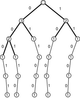
FIG. 3.: Parse tree for the period-$5$ sequence with prime word $00011$. Unvisited paths are not shown. The synchronizing words are shown with bold paths from the start node.

Prime Word	${\bf T}$	${\tau}$
000001	6.97905	3.33333
000011	5.37744	2.83333
000101	5.58496	3.33333
000111	4.83659	2.66667
001011	4.83659	2.66667

TABLE I.: The transient information ${\bf T}$ and synchronization time ${\tau}$ of all five distinct period-$6$ sequences.

To calculate ${\bf T}$ and ${\tau}$ for a given length-$P$ word, we begin by determining the frequency of occurrence of all its subwords. This is done by parsing the word and its $P-1$ cyclic permutations into a tree, whose paths from the root to any node are the subwords and each of whose nodes contain the number of subwords found that lead to it from the root.

An example is shown in Fig. 3. Consider the sequence whose prime word is the length-$5$ word $00011$. We start at the tree root, indicated by the double circle at the top, and follow the leaves labeled with the appropriate symbol. Each time we cross a node we increment the count there by one. We repeat this procedure for all $5$ cyclic permutations of $00011$.

Once the parse tree is built, ${\bf T}$ can be easily and exactly calculated. First, the node counts are turned into probabilities by normalizing — dividing each count by the period $P$. Reading across the tree at level $\ell$ gives the probability of subwords of length $\ell$. In the $P=5$ example considered here, ${\rm Pr}(00)=2/5$, ${\rm Pr}(01)=1/5$, ${\rm Pr}(10)=1/5$, and ${\rm Pr}(11)=1/5$. From these probabilities, the block entropies $H(L)$, and, in turn, ${\bf T}$, follow directly by using Eq. (11) and noting that ${\bf E}=\log_{2}P$ and $h_{\mu}=0$.

Calculating ${\tau}$ is only a bit more involved. After building the parse tree, we reparse each cyclic permutation of the word. As we reparse and proceed down the tree, we monitor the node counts. For each cyclic permutation of the prime word, we follow the corresponding path from the root. When we come to the first node that has a count of $1$, we are synchronized. That is, for the $i^{\rm th}$ cyclic permutation of the word, the level $\ell$ at which we first encounter a node count of $1$ is the synchronization time ${\tau}_{i}$ for that permutation. The average synchronization time ${\tau}$ is then simply:

$${\tau}\,=\,\frac{1}{P}\sum_{i=0}^{P-1}{\tau}_{i}\;.$$ (19)

For the example in Fig. 3, we have

$${\tau}\,=\,\frac{1}{5}(3+3+2+2+2)\,=\,2.4\;.$$ (20)

As for ${\bf T}$, the above method yields an exact value for ${\tau}$.

For example, in Table I we show the results of calculating the transient information ${\bf T}$ and the synchronization time ${\tau}$ for all five distinct period-$6$ sequences. (The reader may find it helpful to verify these results.)

VI Empirical Results

We empirically investigated the behavior of ${\bf T}$ and ${\tau}$ by first exhaustively enumerating all distinct periodic sequences up to and including period $P=23$ and then exactly calculating these two quantities for each using the methods of the previous section. The results are summarized in Figs. 4, 5, 6, 7, and 8. In Table II we show, for periods $2$ through $23$, the number of distinct periodic sequences, the number of distinct ${\bf T}$ and ${\tau}$ values, and the mean, minimum, and maximum ${\bf T}$ and ${\tau}$ values.

Based on these results, one can make a host of observations. First, note that ${\bf T}$ and ${\tau}$ are not the same for all sequences of a given period. This can be seen in our period-$6$ results of Table I, as well as in Figs. 4, 5, and 6. Thus, within a given period, there are many different synchronization behaviors. As noted before, these differences are not accounted for by the entropy rate $h_{\mu}$ and the excess entropy ${\bf E}$, since ${\bf E}$ and $h_{\mu}$ are the same for all sequences with the same period.

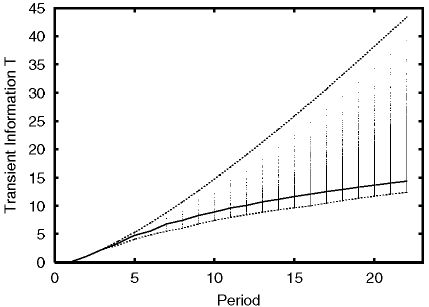
FIG. 4.: Scatter plot of the transient information ${\bf T}$ for all distinct periodic sequences as a function of their prime period $P$, up to $P=22$. The dashed lines are the maximum and minimum ${\bf T}$ values computed analytically; see text. The solid line gives the estimated average ${\bf T}$ value at the given period.

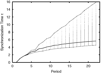
FIG. 5.: Scatter plot of the synchronization time ${\tau}$ for all distinct periodic sequences as a function of their period $P$, up to $P=22$. The dashed lines are the maximum and minimum ${\tau}$ values computed analytically; see text. The solid line gives the estimated average ${\tau}$ value at the given period.

Period	Distinct	Distinct	$\langle{\bf T}\rangle$	${\bf T}_{\rm min}$	${\bf T}_{\rm max}$	Distinct	$\langle{\tau}\rangle$	${\tau}_{\rm min}$	${\tau}_{\rm max}$
$P$	Periodic Sequences	${\bf T}$ Values				${\tau}$ Values
3	1	1	2.25163	2.25163	2.25163	1	1.66667	1.66667	1.66667
4	2	2	3.34436	3.00000	3.68872	2	2.12500	2.00000	2.25000
5	3	3	4.73957	4.07291	5.27291	3	2.80000	2.40000	3.20000
6	5	4	5.52293	4.83659	6.97905	3	2.96667	2.66667	3.33333
7	9	8	6.77183	5.48662	8.78940	8	3.58730	2.85714	4.71429
8	16	13	7.42624	6.00000	10.6907	10	3.72656	3.00000	5.37500
9	28	21	8.27733	6.76598	12.6728	12	4.05556	3.22222	6.22222
10	51	35	8.89152	7.39483	14.7274	22	4.22549	3.40000	6.60000
11	93	53	9.63275	7.94889	16.8480	29	4.50733	3.54545	7.72727
12	170	90	10.0802	8.42155	19.0290	28	4.57157	3.66667	8.41667
13	315	145	10.7162	8.88705	21.2656	49	4.80293	3.76923	9.23077
14	585	261	11.1637	9.29398	23.5540	60	4.89634	3.85714	9.71429
15	1091	484	11.6530	9.66732	25.8906	64	5.03367	3.93333	10.7333
16	2048	610	12.0846	10.0000	28.2725	78	5.13293	4.00000	11.4375
17	3855	1091	12.5298	10.4930	30.6969	104	5.25312	4.11765	12.2353
18	7280	1878	12.9133	10.9359	33.1614	104	5.33134	4.22222	12.7778
19	13797	3205	13.3158	11.3449	35.6640	132	5.43299	4.31579	13.7368
20	26214	5015	13.6772	11.7168	38.2027	143	5.50798	4.40000	14.4500
21	49929	10355	14.0405	12.0774	40.7759	153	5.59134	4.47619	15.2381
22	95325	16031	14.3815	12.4083	43.3818	191	5.66223	4.54545	15.8182
23	182361	27322	14.7179	12.7191	46.0192	207	5.73570	4.60870	16.7391

TABLE II.: The number of distinct periodic sequences, the number of distinct ${\bf T}$ and ${\tau}$ values, and the average, minimum, and maximum ${\bf T}$ and ${\tau}$ values as a function of period, up to $P=23$.

FIG. 6.: The number of distinct periodic sequences, distinct ${\bf T}$ values, and distinct ${\tau}$ values as a function of period $P$. Note the logarithmic scale on the vertical axis.

Second, there are words with the same period that have identical ${\bf T}$ or identical $\tau$ values. This can be seen in Fig. 6, in which we have plotted the count data shown in Table II. The number of distinct ${\bf T}$ and ${\tau}$ values clearly grows less quickly than the total number of distinct periodic sequences. Note also that the number of distinct ${\bf T}$ and ${\tau}$ values grow at different rates. This provides direct evidence that the transient information and the synchronization time measure different qualities. For example, in Table I, note that two sequences have the same ${\tau}$ but different ${\bf T}$’s. The converse also occurs, but much less frequently. There are sequences with the same ${\bf T}$ but different ${\tau}$ values, but this does not occur until $P=12$. As can be seen from both Table II and Fig. 6, ${\tau}$ tends to be substantially more degenerate than ${\bf T}$; ${\tau}$ is somehow a coarser measure of a sequence’s synchronization properties.

Third, note that for a given period there is a considerable range of transient information and synchronization time values. This can be seen in Figs. 4 and 5, where the minimum and maximum ${\bf T}$ and ${\tau}$ values are shown as dashed lines. This suggests that there are significant differences in synchronization behaviors among different sequences with the same period. We will return to the question of minimum and maximum ${\bf T}$ and ${\tau}$ sequences in some detail in Sec. VII.

Another way to view the range of ${\bf T}$ values is found in Fig. 7, in which we plot the distribution of ${\bf T}$ values for period-$16$ and period-$23$ sequences. Note the asymmetry; most ${\bf T}$ values are closer to the minimum ${\bf T}$ than the maximum ${\bf T}$. Similar observations can be made about the distribution of ${\tau}$ values shown in Fig. 8.

FIG. 7.: Normalized histogram of the distribution of ${\bf T}$ values for period-$18$ and period-$23$ sequences.

FIG. 8.: Normalized histogram of the distribution of ${\tau}$ values for period-$18$ and period-$23$ sequences.

Finally, note from Fig. 6 and Table II that the number of distinct ${\tau}$ values is not strictly monotonic with increasing periodicity. Curiously, the number of distinct ${\tau}$ values decreases as the period goes from $11$ to $12$ and it remains constant in going from $P=5$ to $P=6$, while it increases for all other $P$ increases.

VII Minimum, Maximum, and Average ${\bf T}$ and ${\tau}$

Here we develop analytical expressions for the extreme behaviors of the transient information and the synchronization time, and we determine how these extreme values grow asymptotically with period. This analysis allows us to derive a number of important conclusions about which complementary structural features these quantities capture.

First, some notational preliminaries. For a given period, we denote by $\langle{\bf T}\rangle$ the average transient information, averaged over all distinct prime words. Similarly, ${\bf T}_{\rm min}$ and ${\bf T}_{\rm max}$ denote the minimum and maximum ${\bf T}$ values at a given period, respectively. We use similar notation for the average, maximum, and minimum ${\tau}$ values.

A Maximum-${\bf T}$ Sequence

A sequence’s transient information ${\bf T}$ is large if $H(L)$ approaches its asymptotic value of ${\bf E}=\log_{2}P$ slowly. This can be deduced graphically from Figs. 1 and 2. The $H(L)$ curve that grows most slowly is that in which the distribution over subwords is maximally nonuniform, since the entropy of a random variable decreases as its distribution departs from uniformity. For a given period $P$, the sequence with the maximum value of ${\bf T}$ is one consisting of $P\!-\!1$ $0$’s followed by an isolated $1$, since this sequence is the one whose distribution over subwords is as nonuniform as possible. This behavior is seen in one of the period-$8$ sequences shown in Fig. 2.

A direct calculation for the maximal-${\bf T}$ sequence yields:

$${\bf T}_{\rm max}\,=\,\frac{1}{P}\sum_{n=2}^{P}n\log_{2}n\;.$$ (21)

To develop a functional form for ${\bf T}_{\rm max}$ we approximate the sum by an integral. After some work, one obtains,

$${\bf T}_{\rm max}\, \approx \,\frac{1}{\ln(16)P}\left[\,2-P-P^{2}+4\ln(2)\right.$$ (23)

$$\;\;+\;\left.P^{2}\ln(P)+(1\!+\!P)^{2}\ln(1\!+\!P)\,\right]\;.$$

For large $P$, this scales as

$${\bf T}_{\rm max}\,\approx\,\frac{1}{2}P\,{\rm log}_{2}P\;.$$ (24)

The values obtained from Eq. (21) agree with the exact numerical results shown in Table II. In Fig. 9 we plot the approximation of Eq. (23) and compare them with our exact numerical results. As expected, the approximation is quite good and improves at larger $P$.

The synchronization time $\tau$ for the maximum-${\bf T}$ word can be calculated directly by noticing that one is synchronized as soon as one sees a $1$, or after $P-1$ measurements, whichever comes first. One obtains, for large $P$:

$$\tau_{{\rm max\;T}}\sim\frac{P-1}{2}\;,$$ (25)

B Minimum-${\bf T}$ Sequences

The minimum-${\bf T}$ word is particularly easy to analyze when the period is a power of $2$. We begin with this special case and use it to derive a simple form for ${\bf T}_{\rm min}$ as a function of the period.

The sequences with the minimum transient information ${\bf T}_{\rm min}$ correspond to those whose $H(L)$ curves rise most quickly to ${\bf E}$. This is achieved by a sequence whose distribution over subwords, at each subword length, is most nearly uniform and so gives high entropy: the measurements are most informative about the phase.

When the period $P=2^{M}$, where $M$ is an integer, the distribution over subwords for the ${\bf T}_{\rm min}$ sequence is exactly uniform. Words with this property are known as de Bruijn sequences. A binary de Bruijn sequence of order $k$ is a binary circular string containing every binary substring of length $k$ exactly once. For example, the lexicographically smallest order-$3$ binary de Bruijn sequence is $00010111$. Note that this was one of the period-$8$ sequences whose $H(L)$ curve was plotted in Fig. 2. In that figure, the rapid convergence of $H(L)$ to $\log_{2}8=3$ is clearly seen.

FIG. 9.: The minimum, maximum, and average transient information values plotted as a function of period. The solid points are our exact results; the dashed lines are the approximations developed in the text: Eq. (23) for ${\bf T}_{\rm max}$, Eq. (27) for ${\bf T}_{\rm min}$, and Eq. (36) for $\langle{\bf T}\rangle$.

Because every subword appears with equal probability, $H(L)=L$, until $L=\log_{2}P$. That is, $H(L)$ converges linearly to the excess entropy ${\bf E}=\log_{2}P$. In other words, the source appears to be a fair coin until synchrony is achieved. At that time, exact predictability becomes possible. This linear convergence can be seen in Fig. 2. The transient information is thus given by the area between $H(L)$ and $\log_{2}P$;

$${\bf T}_{\rm min}\,=\,\sum_{n=1}^{\log_{2}P}n\;.$$ (26)

Evaluating the sum, one has:

$${\bf T}_{\rm min}\,\approx\,\frac{1}{2}\left(\log_{2}^{2}P+\log_{2}P\right)\;.$$ (27)

Equivalently, since ${\bf E}=\log_{2}P$, we may write this as:

$${\bf T}_{\rm min}\,\approx\,\frac{1}{2}\,{\bf E}\,({\bf E}+1)\;.$$ (28)

This result is exact for all $P$ that are a power of $2$ and serves as an excellent lower bound for $P$’s that are not.

For periods that are not a power of $2$, the minimum-${\bf T}$ words are those for which the distribution over subwords is as uniform as possible. For example, for $P=10$ there are two prime words with minimum ${\bf T}$: $0000101111$ and $0001011101$. Each has ${\bf T}_{\rm min}$ of $7.39483$. Note that for each word, the distribution over subwords of length $1$ is uniform, while the distribution over words of length $2$ is as uniform as can be, given that there are $10$ occurrences of subwords of length $2$; for each, two length-$2$ subwords occur with a frequency of $3/10$ and two occur with a frequency of $2/10$.

We have obtained an analytic expression for ${\bf T}_{\rm min}$ for sequences of general period $P$. The main idea, as stated above, is to distribute the frequencies of the subwords as uniformly as possible. How uniform this distribution is depends on how $2^{L}$ (the number of subwords of length-$L$) divides into the period $P$. Following this line of reasoning, we obtain the following results. Let

$$n_{p}(L)\,\equiv\,\bigg{\lfloor}\,\frac{P}{2^{L}}\,\bigg{\rfloor}\;$$ (29)

and

$$N_{\rm odd}(L)\, \equiv \,P\;{\rm mod}\;2^{L}~{},$$ (30)

$$N_{\rm even}(L)\, \equiv \,2^{L}-N_{\rm odd}(L)~{}.$$ (31)

Here, $\lfloor x\rfloor$ denotes the floor of $x$ — the largest integer smaller than $x$. Similarly, $\lceil x\rceil$ is the ceiling of $x$ — the smallest integer larger than $x$.

The $H(L)$ curve converges to ${\bf E}=\log_{2}P$ by length $L^{*}$, where

$$L^{*}\,\equiv\,\bigg{\lceil}\frac{\log_{2}P}{2}\bigg{\rceil}\,+\,1\;.$$ (32)

Then, we find that the transient information is given by:

$${\bf T}_{\rm min}\,=\,(L^{*}+1)\log_{2}P-\phi\;,$$ (33)

where

$$\phi\, = \,\sum_{n=1}^{L^{*}}\left[-N_{\rm odd}\frac{n_{p}(L)+1}{n}\log_{2}\left(\frac{n_{p}(L)+1}{n}\right)\right.\,$$ (35)

$$\hskip 28.45274pt-\,\left.N_{\rm even}(L)\frac{n_{p}(L)}{n}\log_{2}\left(\frac{n_{p}(L)}{n}\right)\right]\;.$$

Values obtained using Eq. (33) agree with the exact results of Table II.

C Average ${\bf T}$

In Fig. 9 we have also plotted $\langle{\bf T}\rangle$, the average value of the transient information, as a function of the period $P$. These average values were also given in Table II. The average values appear to be well approximated by

$$\langle{\bf T}\rangle\,=\,\frac{1}{2}\log_{2}^{2}P+\log_{2}P\;.$$ (36)

This is an empirical fit. Note that $\langle{\bf T}\rangle$ and ${\bf T}_{\rm min}$ of Eq. (27) are the same to leading order in $P$. This is not surprising, given the asymmetry in the distribution of ${\bf T}$ values evident in Fig. 7.

D Minimum-${\tau}$ Sequences

For a given period $P$, we found that the sequences with the minimum transient information ${\bf T}_{\rm min}$ are the same as the sequences with the minimum synchronization time ${\tau}_{\rm min}$. As noted above, these sequences are those for which the distribution of subwords is most nearly uniform at each subword length. Using this observation, it is possible to derive an analytic expression for ${\tau}_{\rm min}$ among the sequences of period $P$.

As discussed above when considering the minimum-${\bf T}$ word, if $P=2^{M}$, where $M$ is an integer, then the minimum-$\tau$ word is such that all subwords appear with equiprobability. In particular, each subword of length $\log_{2}P$ occurs exactly once. Thus, regardless of the phase in which one begins observing such a sequence, there is no ambiguity about the phase of the sequence after making $\log_{2}P$ observations. For observations shorter than $\log_{2}P$, there will always be some uncertainty about the phase of the process. Thus, the synchronization time is:

$${\tau}_{\rm min}\,=\,\log_{2}P\,=\,{\bf E}\;.$$ (37)

This result is exact when $P=2^{M}$ and is an excellent approximation for other periods.

As mentioned above, ${\bf E}$ is the total phase information stored in the periodic source; it is simply the Shannon entropy of the $P$ possible phases. Recall that the entropy of a random variable sets a lower bound on the number of yes-no questions needed, on average, determine the value of that variable. The synchronization time $\tau$ is equivalent to this average number of yes-no questions — measuring a binary symbol entails asking a yes-no question of the source. Eq. (37) thus shows that the periodic word with the minimum $\tau$ saturates the lower bound set by the entropy.

As was the case for ${\bf T}_{\rm min}$, one can derive an expression for ${\tau}_{\rm min}$ for periods that are not a power of $2$. As with the minimum-${\bf T}$ word, in the minimum-$\tau$ word the distribution over the subwords is as uniform as possible. In the case where $P=2^{M}+1$, $P-2$ phases will synchronize in $M$ observations. The remaining two phases, though, require an additional observation to synchronize; an additional symbol must be seen to distinguish between these two phases. This was the case, for example, for the period-$5$ case considered in Fig. 3. Here, $P=5=2^{2}+1$ and $M=2$. Three of the phases synchronize after two observations, while two phases synchronize after three observations.

Generalizing this observation to $P=2^{M}+N$, we obtain the following result:

$${\tau}_{\rm min}\,=\,\frac{1}{P}\left[\,2N(M\!+\!1)+(P\!-\!2N)M\,\right]\;,$$ (38)

where

$$M\,=\,\bigg{\lfloor}\log_{2}P\bigg{\rfloor}$$ (39)

and

$$N=P\;{\rm mod}\;2^{M}\;.$$ (40)

Eq. (38) can also be written as [17, seq. A061717]:

$${\tau}_{\rm min}\,=\,\frac{1}{P}\bigg{\lceil}\log_{2}P^{P}\bigg{\rceil}\;.$$ (41)

The minimum-${\tau}$ values given by Eq. (38) agree with the exact numerical results shown in Table II. For large $P$, Eq. (41) scales as $\log_{2}P$, in agreement with Eq. (37).

E Maximum-${\tau}$ Sequence

Recall that the maximum-${\bf T}$ sequence consisted of $P\!-\!1$ $0$’s followed by one $1$. For example, the ${\bf T}_{\rm max}$ sequence is $000000001$ for $P=9$. However, this is not the maximum-${\tau}$ sequence. The sequence $000000001$ has an $H(L)$ that grows very slowly, leading to its large ${\bf T}$. However, once one sees a $1$, one is synchronized. Thus, it is possible for an observer to get lucky, see a $1$ after one or two observations and be synchronized quickly. As a result, the expected synchronization time for this sequence is relatively low, only ${\tau}=4.88889$.

In contrast, the sequence with the largest synchronization time for period $9$ is $000010001$ and has ${\tau}=6.2222$. This sequence has the maximum ${\tau}$ due the presence of an additional $1$ which prevents an observer from synchronizing after a single observation; this leads to a larger ${\tau}$.

The maximum-${\tau}$ word for periods $4$-$16$ are given in Table IV. Note that a maximum-${\tau}$ word need not be unique, although we find that it is unique for all periods examined, except for $P=6$.

For $P$ odd, we noticed the maximum-${\tau}$ word takes on a particularly simple form: two $1$’s separated by $(P-3)/2$ zeros. This allows us to determine a simple expression for ${\tau}_{\rm max}$ in this case. We find:

$${\tau}_{\rm max}\,=\,\frac{3}{4}P-\frac{1}{2}-\frac{1}{4P}\,,\;\;P\;{\rm odd}\;.$$ (42)

If the period is even, it is also possible to write down an expression for ${\tau}_{\rm max}$. If $P$ is divisible by $4$, then

$${\tau}_{\rm max}\,=\,\frac{3}{4}P-\frac{1}{2}-\frac{1}{P}\,,\;\;{\rm P\;divisible\;by\;}4\;.$$ (43)

However, if $P$ is divisible by $2$, but not by $4$, then:

$${\tau}_{\rm max}\,=\,\frac{3}{4}P-\frac{1}{2}-\frac{4}{P}\,,\;\;{\rm P\;divisible\;by\;}2\;{\rm and\;not\;}4\;.$$ (44)

Note that, in all cases, to leading order in $P$, ${\tau}_{\rm max}$ grows linearly with $P$:

$${\tau}_{\rm max}\,\sim\,\frac{3}{4}P\;.$$ (45)

Also, in all cases the preceding results agree with the exact values obtained by enumeration and shown in Tables II and IV. Eqs. (42) through (44) were obtained by noting various regularities in the enumeration data and not via a first-principles calculation of the subword statistics.

It is also possible to calculate the transient information ${\bf T}$ for the word that maximizes $\tau$ for the case in which $P$ is odd. Recall that the $\tau_{\rm max}$ word in this case consisted of two $1$’s separated by $(P-3)/2$ zeros. A brute force, direct counting approach yields, for large $P$:

$${\bf T}_{\rm max\;\tau}\,\sim\,\frac{1}{4}P{\bf E}+\frac{P}{2}\;.$$ (46)

FIG. 10.: The minimum, maximum, and average synchronization time plotted as a function of period. The solid points are the exact results from the enumeration; the dashed lines are the approximations developed in the text. The approximation for ${\tau}_{\rm max}$ is that of Eq. (42), which is exact for odd periods. The approximation for ${\tau}_{\rm min}$ is that of Eq. (37), which is exact for periods that are a power of $2$. The approximation for $\langle{\bf T}\rangle$ is the empirical fit of Eq. (47).

F Average Synchronization Time $\langle{\tau}\rangle$

Figure 10 also shows $\langle{\tau}\rangle$, the average synchronization time at a given period, as a function of the period. The dashed line in this figure is an empirical fit:

$$\langle{\tau}\rangle\,\approx\,\frac{5}{4}\log_{2}P\;.$$ (47)

As was the case with the transient information, the average and minimum synchronization times appear to grow asymptotically at the same rate.

VIII Relationships between ${\tau}$ and ${\bf T}$

Throughout the foregoing we have argued that there are important structural differences between distinct periodic sequences at a given period. Moreover, the structural properties captured ${\bf T}$ and ${\tau}$, though both related to synchronization, can be different. Perhaps the differences are not surprising. Based on their definitions these quantities have different interpretations: ${\bf T}$ measures the total uncertainty experienced while synchronizing; ${\tau}$ measures the expected number of observations needed in order to synchronize. To clarify the differences and similarities, in this section we analyze more directly the relationship between ${\bf T}$ and ${\tau}$. We shall see that, while there are relationships between ${\bf T}$ and $\tau$ for the extremal synchronization behaviors, there is a fairly wide range of ${\bf T}$ and $\tau$ combinations possible among different words of the same period.

Period	${\tau}_{\rm max}$	${\tau}_{\rm max}$ word
4	$2.25$	0001
5	$3.2$	00101
6	$3.3333$	000101, 000001
7	$4.71429$	0001001
8	$5.375$	00100101
9	$6.222$	000010001
10	$6.6$	0001001001
11	$7.72727$	00000100001
12	$8.41667$	001010010101
13	$9.23077$	0000001000001
14	$9.71429$	00001000010001
15	$10.7333$	000000010000001
16	$11.4375$	0010101001010101

TABLE III.: Maximum synchronization-time words and ${\tau}_{\rm max}$ values as a function of period $P$.

Function	Minimum	Maximum
${\bf T}$	$\frac{1}{2}\log_{2}^{2}P=\frac{1}{2}{\bf E}^{2}$	$\frac{P}{2}\log_{2}P=\frac{P}{2}{\bf E}$
${\tau}$	$\log_{2}P={\bf E}$	$\frac{3}{4}P$

TABLE IV.: Summary of minimum and maximum ${\bf T}$ and ${\tau}$ behaviors expressed as a function of period $P$ and as a function of the excess entropy ${\bf E}$.

A Extreme Synchronizations

We start by summarizing the behaviors of the minimum and maximum values of the transient information ${\bf T}$ and the synchronization time ${\tau}$ to leading order in the period $P$ in Table IV. Note the enormous range in ${\bf T}$ and ${\tau}$ values. For example, if $P=256$, ${\bf T}_{\rm min}\approx 32$, while ${\bf T}_{\rm max}\approx 1024$. Similarly, for $P=256$, ${\tau}_{\rm min}\approx 8$ while ${\tau}_{\rm max}\approx 192$.

Note that for both the minimum and maximum cases, ${\bf T}$ and $\tau$ are related to each other by:

$${\bf T}\,=\,a\tau{\bf E}\;,$$ (48)

where $a$ is a constant that does not depend on the period $P$. For the minimum-(${\bf T}$, $\tau$) case $a=1/2$ and for the maximum case $a=2/3$. Recall, however, that the maximum-${\bf T}$ word is not the same as the maximum-$\tau$ word. If one uses ${\bf T}_{\rm max}$ and $\tau_{\rm max\;T}$ from Eq. (25) in Eq. (48), one finds $a=1$. And, if one uses ${\bf T}_{\rm max\;\tau}$ and $\tau_{\rm max}$, one find $a=1/3$.

In all cases, note that the ratio of ${\bf T}$ to ${\bf E}$ gives a quantity proportional to $\tau$. This ratio may thus be viewed as setting a characteristic time for synchronization.

B Nonextreme Synchronizations

It turns out, however, that these simple relations mask a wide diversity of synchronization behaviors. Fig. 11, a scatter plot of ${\bf T}$ and ${\tau}$ for all period-$18$ sequences, shows that the relationship between ${\bf T}$ and ${\tau}$ for individual sequences is quite a bit more complicated. For example, recall from the previous section that the maximum-${\bf T}$ sequence does not correspond with the maximum-${\tau}$ sequence. In the Fig. 11, the maximum-${\bf T}$ value is shown by a solid triangle and the maximum-$\tau$ value by a solid square. The minimum-${\bf T}$ and -${\tau}$ sequences are identical, however. This corresponds to the single point in the figure’s lower left corner.

The wide range of points in the scatter plot of Fig. 11 makes it clear that ${\bf T}$ and ${\tau}$ do indeed measure different properties: ${\bf T}$ and ${\tau}$ are not simply rescaled versions of each other. Any simple functional relationship is precluded by the diffuse scatter of points. Said another way, if one lists sequences of a given period in order of increasing ${\bf T}$, this order will not be the same as listing the sequences in order of increasing ${\tau}$.

Although there is considerable spread evident in Fig. 11, there are bounds limiting the range of ${\bf T}$ values at each ${\tau}$.

In fact, one can develop an approximate form for the upper bound in Fig. 11 as follows. Given an arbitrary ${\tau}$ value and the period $P$, we are interested in determining the largest possible ${\bf T}$. Call this maximum value ${\bf T}_{\rm upper}$. Recall that the synchronization time $\tau_{\rm max\;T}$ for the maximum ${\bf T}$ word scales as $P/2$ for large $P$, as shown in Eq. (25). This lets us write

$${\bf T}_{\rm max}\,=\,\frac{1}{2}P{\bf E}\,=\,{\bf E}\tau_{\rm max\;T}\;.$$ (49)

To maximize ${\bf T}$ for a given $\tau$, assume that the given $\tau$ is that which maximizes ${\bf T}$. Then, using the above equation, we see that ${\bf T}_{\rm upper}\propto{\bf E}\tau$. That is, the slope of the linear upper bound is ${\bf E}$. To get the full equation of the line, we require that it go through the minimum-$({\tau},{\bf T})$ point on the lower left hand corner of Fig. 11. Using Eqs. (27) and (37) for the values of ${\bf T}_{\rm min}$ and ${\tau}_{\rm min}$, respectively, we then obtain

$${\bf T}_{\rm upper}\,\approx\,{\bf E}\,[{\tau}-\frac{1}{2}({\bf E}-1)]\;.$$ (50)

This upper bound is plotted in Fig. 11, with ${\bf E}={\rm log}_{2}18\approx 4.1699\ldots$. This upper bound is only approximate because the minimum-($\tau,{\bf T}$) values used in its calculation are the asymptotic values for large $P$. The bound is also approximate because the relationship in Eq. (49), which is true for the maximum-${\bf T}$ sequence (the solid triangle in the figure), is assumed to hold for all sequences. Despite these approximations, the linear upper bound appears to fit the data quite well, as shown in Fig. 11.

FIG. 11.: A scatter plot of ${\bf T}$ versus ${\tau}$ for all period-$18$ sequences. The upper bound is that of Eq. (50) and the lower bound is that of Eq. (52). The solid triangle is the $({\tau},{\bf T})$ point for the ${\bf T}_{\rm max}$ sequence; the solid square denotes the ${\tau}_{\rm max}$ sequence.

A similar line of reasoning allows us to form a lower bound ${\bf T}_{\rm lower}$ for the smallest possible ${\bf T}$, given a value of $\tau$ and the period $P$. From Eqs. (28) and (37), for large $P$ we know that ${\bf T}_{\rm min}\approx\frac{1}{2}E^{2}$ and $\tau_{\rm min}\approx{\bf E}$. This gives us

$${\bf T}_{\rm min}\,=\,\frac{1}{2}{\bf E}\tau_{\rm min}\;.$$ (51)

To minimize ${\bf T}$, we assume that the given $\tau$ is the minimum $\tau$. This tells us that the slope of a linear lower bound is $\frac{1}{2}{\bf E}$. Requiring the line to go through the minimum $\tau,{\bf T}$ point yields

$${\bf T}_{\rm lower}\,=\,\frac{1}{2}\tau+\frac{1}{2}E^{2}\;.$$ (52)

This is only an approximate bound, for the same reasons that ${\bf T}_{\rm upper}$ is approximate. Eq. (52) is plotted in Fig. 11. It is indeed a lower bound, but the bound is not very tight.

IX Discussion and Conclusion

We began by introducing two measures of how difficult it is to synchronize to a sequence: the transient information ${\bf T}$, an information-theoretic measure of the total uncertainty experienced by an observer during the synchronization process; and the synchronization time ${\tau}$, the number of symbols an observer expects to measure before it is synchronized. We exactly calculated ${\bf T}$ and ${\tau}$ for all synchronization-distinct periodic sequences up to and including period $23$. We also derived a handful of analytic expressions and approximations for the minimum, maximum, and average ${\bf T}$ and ${\tau}$ as a function of period.

Our results show that there are many structural differences between periodic sequences, even within sequences of the same period. These differences are simply not captured by commonly used information theoretic measures, such as the entropy rate and the excess entropy. Are all periodic sequences of a given period the same from an information-theoretic standpoint? The answer we gave here is “no”; the recently introduced transient information, in fact, captures the information-theoretic differences between sequences of a given period. Are there structural differences between different periodic sequences of the same period? We showed that the answer is “yes” and argued that the differences are significant. Are there distinct classes of periodic sequence? Again, we provided a positive answer, partly by contrasting properties captured by the transient information with a sequence’s group theoretic properties and its synchronization time. The latter measures the average number of observations needed to synchronize to the sequence and, for a given sequence at a given period, this number was neither the same nor simply proportional to the transient information. Nonetheless, at a coarse level, the leading-order approximations we developed provide simple and direct links between the three different concepts of phase memory ${\bf E}$, synchronization time ${\tau}$, and the total uncertainty experienced during synchronization ${\bf T}$.

There are a number of areas in which our results may find application. For one, recognizing the phases of long periodic sequences of the type investigated here is a key technology for current and future large-scale satellite-to-satellite communication systems. These multiagent systems require extremely accurate and robust satellite-to-satellite synchronization [19] generally for coordination in signal processing and navigation and specifically for estimating inter-satellite signal delays and distances. Synchronization between two satellites is effected by one transmitting a very long ($P\sim 1,000$) and known binary periodic sequence. The receiver then infers the phase, using a hierarchical correlation algorithm adapted to account for noise corruption of individual symbols during transmission. It turns out that the long periodic acquisition sequences are aperiodic sequences formed from relatively “prime” short aperiodic sequences. In fact, the synchronization properties of the component sequences and the composite acquisition sequence determine bounds on the computational effort and noise robustness that can be achieved by the receiver’s detection system. We conjecture that the transient information of the acquisition sequence is a key parameter determining these properties.

More generally, these results bear on any situation in which an intelligent agent needs to learn the phase of a periodic component in its environment’s behavior; cf. Ref. [8]. This arises in multiagent systems if an agent needs to know where it is in a physical environment that varies periodically in space or time, if it needs to adjust its behavior in response to the repetitive behavior of other agents, or if a collective decision requires coordinated information processing.

Finally, we mention several open questions and directions for future work. First, do these results hold if the synchronization process is noisy and bits flip occasionally? They should extend relatively directly to a class of “noisy-periodic” processes in which one or several symbols in a periodic sequence are random. However, can these results be extended to the full class of finite-memory sources? For a further discussion of the synchronization scenario in a setting not restricted to periodic sequences see Refs. [5] and [8].

Second, one may view those sequences at a given period with the same ${\bf T}$ as forming an equivalence class. Recall that distinct periodic sequences were defined by the group $S_{k}\times C_{P}$. These are the equivalence classes of zero entropy rate, finite excess entropy sequences. But what new algebra or symmetry group of periodic sequences characterizes those sequences that are equally hard to synchronize to, as measured by ${\bf T}$ or $\tau$? If we can characterize identical ${\bf T}$ or $\tau$ sequences in terms of a symmetry group or algebra, it should be possible to obtain an analytic expression for the number of distinct ${\bf T}$ or $\tau$ values at a given period.

Third, as noted above, Titsworth [18] pointed out that Eq. (18) gives the number of distinct finite-state machines needed to generate all sequences of a given prime period. The picture is that starting in a different state of such a machine gives the cyclic permutations, while exchanging the output symbols gives the permutation $0\leftrightarrow 1$. Titsworth does not comment on the structure of the synchronizing states of these machines. To account for synchronization one wants each finite-state machine to have a unique start state that corresponds to the condition of an observer not knowing in which phase a periodic sequence starts. It turns out that $\epsilon$-machines [20, 21, 22] capture this synchronizing structure in their transient states, and these in turn determine ${\bf T}$. Moreover, this is true for both periodic and random sources. Based on these observations we conjecture that the number of distinct ${\bf T}$ values for a given period is the number of distinct $\epsilon$-machines needed to recognize all periodic sequences of a given prime period. That is, we conjecture that those sequences with the same ${\bf T}$ value have the same transient $\epsilon$-machine structure, up to edge relabeling.

In summary, we analyzed what is arguably the simplest class of sequences: zero entropy rate, finite-period sequences. The sequences represent behaviors that are often ignored in many fields as being too simple. As we demonstrated, however, their structural complexity and synchronization properties are rich and subtle. Within a given period, there are large differences in structural complexity, as measured by the transient information ${\bf T}$ and the synchronization time ${\tau}$. Thus, even simple periodic systems are surprisingly complex.

REFERENCES

- [1] C. E. Shannon and W. Weaver. The Mathematical Theory of Communication. University of Illinois Press, Champaign-Urbana, 1962.
- [2] T. M. Cover and J. A. Thomas. Elements of Information Theory. John Wiley & Sons, Inc., 1991.
- [3] J. P. Crutchfield and N. H. Packard. Symbolic dynamics of noisy chaos. Physica D, 7:201–223, 1983.
- [4] P. Grassberger. Toward a quantitative theory of self-generated complexity. Intl. J. Theo. Phys., 25(9):907–938, 1986.
- [5] J. P. Crutchfield and D. P. Feldman. Regularities unseen, randomness observed: Levels of entropy convergence. Chaos, 2001. arXiv.org/abs/cond-mat/0102181. Chaos, In Press.
- [6] K. Lindgren and M. G. Norhdal. Complexity measures and cellular automata. Complex Systems, 2(4):409–440, 1988.
- [7] W. Li. On the relationship between complexity and entropy for Markov chains and regular languages. Complex Systems, 5(4):381–399, 1991.
- [8] J. P. Crutchfield and D. P. Feldman. Synchronizing to the environment: Information theoretic constraints on agent learning. Advances in Complex Systems, 4:251–264, 2001.
- [9] R. M. Gray. Entropy and Information Theory. Springer-Verlag, New York, 1990.
- [10] W. Ebeling. Prediction and entropy of nonlinear dynamical systems and symbolic sequences with LRO. Physica D, 109:42–52, 1997.
- [11] W. Bialek, I. Nemenman, and N. Tishby. Predictability, complexity, and learning. physics/0007070v2, 2000.
- [12] R. Shaw. The Dripping Faucet as a Model Chaotic System. Aerial Press, Santa Cruz, California, 1984.
- [13] I. Nemenman. Information Theory and Learning: A Physical Approach. PhD thesis, Princeton University, 2000.
- [14] N. J. Fine. Classes of periodic sequences. Illinois Journal of Mathematics, 2:285–302, 1958.
- [15] E. N. Gilbert and J. Riordan. Symmetry types of periodic sequences. Illinois J. Math., 5:657–665, 1961.
- [16] Combinatorial object server. http://www.theory.csc.uvic.ca/~cos/root.html.
- [17] N. J. A. Sloan. The on-line encyclopedia of integer sequences. http://www.research.att.com/~njas/sequences/index.html. Individual integer sequences in the encyclopedia are referenced by Annnnnn.
- [18] R. C. Titsworth. Equivalence classes of periodic sequences. Illinois J. Math., pages 266–270, 1964.
- [19] J. L. Massey. Noisy sequence acquisition with minimum computation. Lecture Notes, Ulm Winter School, 2000.
- [20] J. P. Crutchfield and K. Young. Inferring statistical complexity. Phys. Rev. Lett., 63:105–108., 1989.
- [21] J. P. Crutchfield. The calculi of emergence: Computation, dynamics, and induction. Physica D, 75:11–54, 1994.
- [22] C. R. Shalizi and J. P. Crutchfield. Computational mechanics: Pattern and prediction, structure and simplicity. Journal Statistical Physics, 104:819–881, 2001.