Scarred eigenstates for quantum cat maps of minimal periods

Abstract

In this paper we construct a sequence of eigenfunctions of the “quantum Arnold’s cat map” that, in the semiclassical limit, show a strong scarring phenomenon on the periodic orbits of the dynamics. More precisely, those states have a semiclassical limit measure that is the sum of $1/2$ the normalized Lebesgue measure on the torus plus $1/2$ the normalized Dirac measure concentrated on any a priori given periodic orbit of the dynamics. It is known (the Schnirelman theorem) that “most” sequences of eigenfunctions equidistribute on the torus. The sequences we construct therefore provide an example of an exception to this general rule. Our method of construction and proof exploits the existence of special values of $\hbar$ for which the quantum period of the map is relatively “short”, and a sharp control on the evolution of coherent states up to this time scale. We also provide a pointwise description of these states in phase space, which uncovers their “hyperbolic” structure in the vicinity of the fixed points and yields more precise localization estimates.

1 Introduction

One of the main problems in quantum chaos is the understanding of the semiclassical behaviour of the eigenfunctions of quantum dynamical systems having a chaotic classical limit. The main theorem in this context is the Schnirelman theorem [Sc, CdV, Z1, HMR, BouDB]. It roughly states that “most” eigenfunctions equidistribute on the available phase space in the classical limit. This leaves open the question of the existence of exceptional sequences of eigenfunctions with a different limit. In the case of “hard chaos” (uniformly hyperbolic systems), numerical computations have shown the presence of “scars” on certain eigenfunctions [He], i.e. a visual enhancement of the wavefunction on an unstable periodic orbit. Up to now all theories of this phenomenon have required some kind of averaging over a (semiclassically large) set of eigenfunctions [Bog, Ber, He, KH]. In addition, scarring is often described in the physics literature as a weak type of localization, compatible with Schnirelman’s (measure-theoretic) equidistribution, as opposed to “strong scarring” [RS], which implies that the limiting measure has a component supported on a periodic orbit and therefore does not equidistribute. We show in this paper that, for the quantized “Arnold’s cat map”, strongly scarred sequences do indeed exist for any periodic orbit (more generally, for any finite union of periodic orbits). This is, to the best of our knowledge, the first example of this kind in hyperbolic systems. A construction of exceptional sequences of eigenfunctions not equidistributing in the semiclassical limit was recently announced [CKS] for the quantization of certain ergodic piecewise affine transformations on the torus, but these do not correspond to “scars” since the systems in question have no periodic orbits.

Our construction is based on intuitively clear ideas that we now briefly sketch. For unfamiliar notation, we refer to Sections 2–4. Precise statements of our results will be given below.

Let $M\in$ SL$(2,\mathbb{Z})$ be a hyperbolic automorphism of the 2-dimensional torus $\mathbb{T}$ and $\hat{M}$ its quantization on the $N$-dimensional quantum Hilbert space ${\mathcal{H}}_{N,\theta}$, where $2\pi\hbar N=1$. We will construct strongly scarred quasimodes of $\hat{M}$ that, for certain values of $N$, will be shown to be eigenfunctions. For that purpose we will use three ingredients. First, the time-energy uncertainty relation in the following simple form ($T\in\mathbb{N},\phi\in\mathbb{R}$):

$$\parallel(\hat{M}-\rm e^{{\rm i}\phi}\hat{I})\sum_{t=-T}^{T-1}\rm e^{-{\rm i}\phi t}\hat{M}^{t}\parallel=\parallel\rm e^{-2{\rm i}\phi T}\hat{M}^{2T}-\hat{I}\parallel\leq 2.$$ (1)

Second, precise estimates on intuitively clear phase space localization properties of coherent states. Third, a remark on the quantum period of $\hat{M}$ [BonDB1] (Section 8).

Let $x_{0},x_{1}=Mx_{0},\dots,x_{\tau}=M^{\tau}x_{0}=x_{0}$ be a periodic orbit of period $\tau$ of $M$. Let $|x_{0},\tilde{c}_{0},\theta\rangle$ be a “squeezed” coherent state in ${\cal H}_{N,\theta}$ centered on the point $x_{0}$ and consider $\hat{M}^{t}|x_{0},\tilde{c}_{0},\theta\rangle$ for $t\in\mathbb{Z}$. Note first that this state is still a squeezed coherent state and that, for small enough $t$, it is localized around $x_{t}$. In fact, the support of the Husimi function of this state is an ellipse stretched along the unstable direction of the dynamics through the point $x_{t}$, with its major axis roughly of size $\sqrt{\hbar}\rm e^{\lambda t}$, where $\lambda$ is the (positive) Lyapounov exponent of the dynamics (Section 4). Introducing the Ehrenfest time $T=\frac{|\ln\hbar|}{\lambda}$, the support is therefore microscopic as long as $t\leq(1-\epsilon)T/2$. For longer times, between $T/2$ and $T$, the support of the Husimi function of $\hat{M}^{t}|x_{0},\tilde{c}_{0},\theta\rangle$ starts to wrap around the torus and it was shown in [BonDB1] that it equidistributes on that time scale.

We shall consider the “discrete time quasimode”

$$|\Phi^{\rm disc}_{\phi}\rangle=\sum_{t=-T}^{T-1}\rm e^{-{\rm i}\phi t}\hat{M}^{t}|x_{0},\tilde{c}_{0},\theta\rangle=\sum_{j=1}^{4}|\Phi_{j,\phi}^{\rm disc}\rangle$$ (2)

and its “components”

$$|\Phi_{j,\phi}^{\rm disc}\rangle=\sum_{t=-T+(j-1)\frac{T}{2}}^{-T+j\frac{T}{2}-1}\rm e^{-{\rm i}\phi t}\hat{M}^{t}|x_{0},\tilde{c}_{0},\theta\rangle.$$ (3)

We note that similar states were considered before in the study of scars, see for instance [dPBB, KH] and references therein.

Figure 1: Partition of the time interval $[-T,T]$ into four equal parts, and of the quasimode $|\Phi_{\phi}\rangle$ into corresponding components.

We shall introduce a “continuous time” version $|\Phi^{\rm cont}_{\phi}\rangle$ of those quasimodes later. We will write $|\Phi_{\phi}\rangle$ in statements true for both the discrete and continuous time quasimodes.

Let us for simplicity concentrate on the case where $x_{0}=0,\tau=1$. Our crucial technical estimate (Section 4–Proposition 1) says that there exists $C>0$ so that

$$\langle\tilde{c}_{0},\theta\mid\hat{M}^{t}\mid\tilde{c}_{0},\theta\rangle=\frac{1}{\sqrt{\cosh(\lambda t)}}+I(t),\;{\rm with}\>|I(t)|\leq C\rm e^{-\lambda(T-\frac{|t|}{2})}.$$ (4)

This implies rather easily (Proposition 2) the existence of a smooth, strictly positive function $S_{1}(\phi,\lambda)$ so that

$$\langle\Phi_{\phi}\mid\Phi_{\phi}\rangle\sim 2S_{1}(\phi,\lambda)T.$$

Using (1) one concludes readily that

$$\parallel(\hat{M}-\rm e^{{\rm i}\phi}\hat{I})|\Phi_{\phi}\rangle_{n}\parallel\leq\sqrt{\frac{2}{{S_{1}(\phi,\lambda)T}}}\left(1+\frac{\mathcal{O}(1)}{S_{1}(\phi,\lambda)T}\right)\,,$$ (5)

justifying the name “quasimode”. Here we used the notation $|\psi\rangle_{n}=|\psi\rangle/\sqrt{\langle\psi|\psi\rangle}$ for any non-zero $|\psi\rangle\in{\mathcal{H}}_{N,\theta}$.

To analyze the phase space properties of the above quasimodes, we first show as a further consequence of (4) that the four states $|\Phi_{j,\phi}\rangle$ have the same norm, asymptotically proportional to $\sqrt{T}$ as $\hbar$ goes to $0$ and that they are asymptotically orthogonal in the semiclassical limit. In fact, this is easily understood intuitively by noting for example that the Husimi function of $|\Phi_{1,\phi}\rangle$ is supported along the stable manifold of the periodic orbit, and that of $|\Phi_{4,\phi}\rangle$ along the unstable one, so that they have essentially disjoint supports, which is at the origin of their orthogonality. To put it differently, since the unstable and stable manifolds intersect at homoclinic points, our results show that the contribution of these intersections in the phase space integral expressing the overlap $\langle\Phi_{1,\phi}|\Phi_{4,\phi}\rangle$ is small for small $\hbar$. Note that although the homoclinic interferences do not contribute significantly to the above integral, they are nevertheless clearly visible on the pointwise behaviour of the Husimi distribution of $|\Phi_{\phi}\rangle$, which is represented in Figure 2 and that will be further studied in Section 6 (for “continuous time” quasimodes). The pointwise estimates obtained there will show that the Husimi density concentrates along “classical hyperbolas” asymptotic to the stable and unstable manifolds; they will at the same time provide estimates on the rate of convergence to the limit measure, as well as other localization indicators (namely, $L^{s}$ norms of the Husimi density).

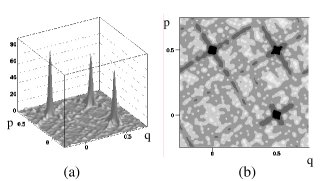
Figure 2: Husimi distribution of the state $|\Phi_{\phi}\rangle_{n}$, constructed for the cat map (21) on the orbit of period $3$ starting from $x_{0}=(0,0.5)$. The quantum parameters read $N=1/(2\pi\hbar)=500$, $\phi=0$. (a): 3D plot on a linear scale. (b): 2D plot in logarithmic scale (darker = higher values).

It is furthermore clear from the previous discussion on the phase space localization properties of the evolved coherent states that $|\Phi_{1,\phi}\rangle$ and $|\Phi_{4,\phi}\rangle$ are sums of states that equidistribute on the torus, whereas $|\Phi_{2,\phi}\rangle$ and $|\Phi_{3,\phi}\rangle$ are sums of states that localize on the periodic orbit. One therefore expects (and we shall prove in Sections 5–7) that

$$\lim_{\hbar\to 0}\ {}_{n}\!\langle\Phi_{j,\phi}|\hat{f}|\Phi_{j,\phi}\rangle_{n}=\int_{\mathbb{T}}f(x)dx\qquad{\rm if}\ j=1,4,$$

and that

$$\lim_{\hbar\to 0}\ {}_{n}\!\langle\Phi_{j,\phi}|\hat{f}|\Phi_{j,\phi}\rangle_{n}=\frac{1}{\tau}\sum_{i=0}^{\tau-1}f(x_{i})\qquad{\rm if}\ j=2,3.$$

Here $\hat{f}$ is either the Weyl or anti-Wick quantization of $f\in C^{\infty}(\mathbb{T})$. In other words, the Wigner and hence also the Husimi function of $|\Phi_{2,3,\phi}\rangle$ converge (weakly) to the Dirac measure on the periodic orbit, whereas the ones of $|\Phi_{1,4,\phi}\rangle$ equidistribute, i.e. converge to the Lebesgue measure. This suggests grouping these states two by two, defining:

$$|\Phi_{{\rm erg},\phi}\rangle=|\Phi_{1,\phi}\rangle+|\Phi_{4,\phi}\rangle\;\ {\rm and}\;\ |\Phi_{{\rm loc},\phi}\rangle=|\Phi_{2,\phi}\rangle+|\Phi_{3,\phi}\rangle.$$ (6)

Using the above information we shall finally prove (Propositions 7 and 12) that, for any $\phi\in[-\pi,\pi]$,

$$\lim_{\hbar\to 0}\ {}_{n}\!\langle\Phi_{\phi}|\hat{f}|\Phi_{\phi}\rangle_{n}=\frac{1}{2}\int_{\mathbb{T}^{2}}f(x)dx+\frac{1}{2}\left[\frac{1}{\tau}\sum_{j=0}^{\tau-1}f(x_{j})\right].$$ (7)

In other words, the semiclassical limit measure of the sequence of quasimodes $|\Phi_{\phi}\rangle_{n}$ is the measure

$$\frac{1}{2}dx+\frac{1}{2}\left[\frac{1}{\tau}\sum_{j=0}^{\tau-1}\delta_{x_{j}}\right].$$

This shows that the quasimodes $|\Phi_{\phi}\rangle_{n}$ are strongly scarred.

We then conclude using a particular property of the quantum period of $\hat{M}$. We recall that the quantum cat map $\hat{M}$ has an $\hbar$ dependent “quantum period” $P$, i.e. $\hat{M}^{P}=\rm e^{-{\rm i}\varphi}\hat{I}$ for some $\varphi\in[0,2\pi[$. The eigenvalues of $\hat{M}$ on ${\cal H}_{N,\theta}$ are therefore all of the form $\rm e^{-{\rm i}\phi_{j}}$, with $\phi_{j}=\varphi/P+2\pi j/P$, $j=1,\dots,P$. Note that $P$ plays the role here of the Heisenberg time of the system, since $\Delta\phi_{j}\sim 1/P$. Since, for general $\hbar$, the quantum period $P$ is of order $\hbar^{-1}$ [Ke], it is considerably longer than the Ehrenfest time $T$, which grows only logarithmically in $\hbar^{-1}$. Nevertheless, developing an argument in [BonDB1], we will show that, for any hyperbolic matrix in SL$(2,\mathbb{Z})$ there exists a subsequence $(\hbar_{k})_{k\in\mathbb{N}}$ of values of $\hbar$ tending to zero for which $P=2T+\mathcal{O}(1)$ (see also [KR2]). For those values the Heisenberg and Ehrenfest times of the system coincide and the $|\Phi_{\phi}\rangle_{n}$ therefore constitute a sequence of eigenfunctions of $\hat{M}$ that strongly scar, provided $\phi=\phi_{j}$ for some $j\in\{1\dots P\}$. It should be noted that, for the values of $\hbar$ considered, the number of distinct eigenvalues $\phi_{j}$ is of order $|\ln\hbar|$, so that the eigenvalue degeneracy is very large, namely of order $(\hbar|\ln\hbar|)^{-1}$.

Our main result can finally be summarized as follows:

Theorem 1.

Let $M$ and $(\hbar_{k})_{k\in\mathbb{N}}$ be as above. Let $0\leq\beta\leq 1/2$ and let $\mathcal{P}=\{x_{0},\ldots,x_{\tau-1}\}$ be a periodic orbit of $M$. Then there exists a sequence $(\psi_{j_{k}})_{k\in\mathbb{N}}$ of eigenfunctions of $\hat{M}$ on $\mathcal{H}_{N_{k},\theta}$ with the property that, for all $f\in C^{\infty}(\mathbb{T}^{2})$,

$$\lim_{k\to\infty}\ {}_{n}\!\langle\psi_{k}|\hat{f}|\psi_{k}\rangle_{n}=\beta\frac{1}{\tau}\sum_{j=0}^{\tau-1}f(x_{j})+(1-\beta)\int_{\mathbb{T}^{2}}\ f(x)\,dx.$$ (8)

Our result helps to complete the picture of the semiclassical eigenfunction behaviour of quantized toral automorphisms known to date. Indeed, beyond the general Schnirelman theorem for these models [BouDB] the following results are known. First, suppose $M$ is of “checkerboard form”, meaning $AB\equiv 0\equiv CD\bmod 2$. Then all eigenfunctions of $\hat{M}$ semiclassically equidistribute, provided one takes the limit along a density one subsequence of values of $N$ [KR2], for which the quantum period is larger than $\sqrt{N}$. Note that this sequence excludes the values $N_{k}$ for which the period is very short. Second, it is shown in [KR1, Me] that for such $M$ there exists a basis of eigenfunctions that equidistribute as $N$ tends to infinity, without restrictions on $N$. This basis is constructed as a common eigenbasis for $\hat{M}$ and its “quantum symmetries”, which are shown in [KR1] to be sufficiently numerous to drastically reduce (if not to lift) the degeneracies of the eigenvalues. Finally, one may wonder if it would be possible to construct a sequence of eigenfunctions of $\hat{M}$ that has as a limit measure

$$\beta\frac{1}{\tau}\sum_{j=0}^{\tau-1}\delta_{x_{j}}+(1-\beta)dx,$$

with $\beta>1/2$. It is proven in [FN1] that this is impossible, so that the above quasimodes are in a sense maximally localized (the bound $\beta>(\sqrt{5}-1)/2\cong 0.62$ had been previously obtained by [BonDB2]).

2 Linear dynamics on the plane

In this section we recall some known results we will need in the sequel. For details not given here we refer to [F].

2.1 Classical linear flow

The most general quadratic Hamiltonian on $\mathbb{R}^{2}$ is ($\alpha,\beta,\gamma\in\mathbb{R})$:

$$H(q,p)=\frac{1}{2}\alpha q^{2}+\frac{1}{2}\beta p^{2}+\gamma qp.$$ (9)

Assuming $\gamma^{2}>\alpha\beta$, $H$ generates a hyperbolic flow $x(t)=(q(t),p(t))$ on $\mathbb{R}^{2}$, given by $x(t)=M{(t)}x(0)\ (t\in\mathbb{R})$, where for each $t\not=0$, $M(t)$ is a hyperbolic matrix in SL$(2,\mathbb{R})$. Explicitly, for $t=1$

$$M\stackrel{{\scriptstyle\rm def}}{{=}}M(1)=\left(\begin{array}[]{cc}A&B\\ C&D\end{array}\right)\in{\rm SL}\left(2,\mathbb{R}\right),$$ (10)

i.e. $AD-BC=1$, and

$$\left\{\begin{array}[]{ll}A=\cosh\lambda+\frac{\gamma}{\lambda}\sinh\lambda&B=\frac{\beta}{\lambda}\sinh\lambda\\ C=-\frac{\alpha}{\lambda}\sinh\lambda&D=\cosh\lambda-\frac{\gamma}{\lambda}\sinh\lambda\end{array}\right.$$ (11)

where $\lambda=\sqrt{\gamma^{2}-\alpha\beta}>0$ is the Lyapounov exponent. Note that $M$ has two real eigenvalues $\rm e^{\pm\lambda}$ and hence two real eigenvectors corresponding to an unstable and a stable direction for the dynamics. They have respective slopes $s_{+}=\tan\psi_{+},s_{-}=\tan\psi_{-}$. Clearly, any hyperbolic matrix $M\in$ SL$(2,\mathbb{R})$ with Tr$M>2$ is of the above form for a unique $\alpha,\beta,\gamma$ (the case Tr$M<-2$ is treated by using the map $-M$). The expressions in (10)–(11) still make sense in the elliptic case, when $\gamma^{2}<\alpha\beta$ and $-2<$Tr$M<2$. In terms of the complex coordinate $z=\frac{1}{\sqrt{2}}\left(q+{\rm i}p\right)$, the Hamiltonian in (9) reads

$$H=\frac{c}{2}z^{2}+\frac{\overline{c}}{2}\overline{z}^{2}+bz\overline{z},\ {\rm with}\ b=\frac{1}{2}\left(\alpha+\beta\right)\in\mathbb{R},\ c=\frac{1}{2}\left(\alpha-\beta\right)-{\rm i}\gamma\in\mathbb{C}.$$ (12)

and $\lambda=\sqrt{\left|c\right|^{2}-b^{2}}.$ We shall write $M_{(c,b)}$ for the matrix $M$ constructed via (10)–(12), whenever $b^{2}\not=|c|^{2}$.

We will make use of the following convenient decomposition of a general hyperbolic matrix $M$ (Tr$M>2$). We first introduce some notation. For $\mu\in\mathbb{R}_{+}$ we define:

$$D(\mu)\stackrel{{\scriptstyle\rm def}}{{=}}M_{(c=-{\rm i}\mu,b=0)},\quad B(\mu)\stackrel{{\scriptstyle\rm def}}{{=}}M_{\left(c=-\mu,b=0\right)},\quad R(\mu)\stackrel{{\scriptstyle\rm def}}{{=}}M_{(c=0,b=-\mu)}.$$

Clearly, $D(\mu)$ is hyperbolic, with the $q$ and $p$ axes as unstable and stable axes. $B(\mu)$ is also hyperbolic, with eigenaxes forming angles $\psi_{+}=\frac{1}{2}\arg(-{\rm i}\bar{c})=\frac{\pi}{4}=-\psi_{-}$ with the horizontal. $R(\mu)$, on the other hand, is just a rotation of angle $\mu$ and hence elliptic. Any hyperbolic matrix $M_{(c,b)}$ as in (10) can be decomposed as:

$$M_{(c,b)}=QD(\lambda)Q^{-1},\ {\rm with}\ Q=R(b_{1})B(b_{2}),$$ (13)

where $b_{1}\in\left[-\frac{\pi}{2},\frac{\pi}{2}\right]$, $b_{2}\in\mathbb{R}$ are defined as follows. We denote by $\phi_{1}\in\left[-\frac{\pi}{2},\frac{\pi}{2}\right]$ the angle between the $q$ axis and the bisector between the stable and unstable axes of $M_{(c,b)}$, and by $\phi_{2}\in\left]0,\frac{\pi}{4}\right]$ the angle between the bisector and the stable axis of $M_{(c,b)}$ (Figure 3). In terms of those, one has:

$$\sinh\left(2b_{2}\right)=\frac{1}{\tan\left(2\phi_{2}\right)},\qquad b_{1}=\phi_{1}-\frac{\pi}{4}.$$ (14)

Figure 3: Decomposition of the general linear hyperbolic map $M_{(c,b)}$ as in (13).

This last decomposition has the following interpretation. The general hyperbolic map $M_{(c,b)}$ is obtained from the special case $D(\lambda)$ ($\lambda=\sqrt{|c|^{2}-b^{2}}>0$) by a change of coordinates $Q$ yielding a transformation from the $(q,p)$ frame into the unstable-stable frame. The unstable (respectively stable) direction is given by the vectors ${v}_{+}=Q\,{e}_{q}$, ${v}_{-}=Q\,{e}_{p}$ (which are, in general, not normalized). Above, we decomposed $Q$ into the transformation $B(b_{2})$ which changes the angle between the stable and unstable axis, and the rotation $R(b_{1})$ which rotates the whole frame (Figure 3).

We finally remark, for later purposes, that there exists another decomposition: given $M\in\mathrm{SL}(2,\mathbb{R})$, $\exists!\tilde{c}\in\mathbb{C}$, $\mu\in]-\pi,\pi]$ so that

$$M=M_{(\tilde{c},0)}R(\mu).$$ (15)

2.2 Linear quantum dynamics

In terms of the usual annihilation and number operators $a=\frac{1}{\sqrt{2\hbar}}\left(\hat{q}+i\hat{p}\right)$, and $\hat{n}=\frac{1}{2}\left(a^{\dagger}a+aa^{\dagger}\right),$ the Weyl (or canonical) quantization of $H$ in (9) is defined as the self-adjoint operator $\hat{H}$ on $L^{2}(\mathbb{R})$ given by:

$$\hat{H}=\frac{1}{2}\alpha\hat{q}^{2}+\frac{1}{2}\beta\hat{p}^{2}+\gamma\frac{1}{2}\left(\hat{q}\hat{p}+\hat{p}\hat{q}\right)=\hbar\left(\frac{c}{2}a^{2}+\frac{\overline{c}}{2}a^{\dagger 2}+b\hat{n}\right).$$ (16)

The quantum evolution operator for time $t=1$ which corresponds to $M_{(c,b)}$ is then:

$$\hat{M}_{(c,b)}=\exp\left\{-{\rm i}\frac{\hat{H}}{\hbar}\right\}.$$ (17)

The quantization of the matrix $-M_{(c,b)}=M_{(c,b)}R(\pi)$ can be defined as $\hat{M}_{(c,b)}\hat{P}=\hat{P}\hat{M}_{(c,b)}$ where $\hat{P}=-{\rm i}\hat{R}(\pi)$ is the parity operator. The unitary operators $\hat{M}_{(c,b)}$, $\hat{M}_{(c,b)}\hat{P}$ yield a projective representation of SL$(2,\mathbb{R})$ (which resembles the metaplectic representation). We will in most of the paper omit to indicate the $\hbar$-dependence of the operators $\hat{H}$ and $\hat{M}_{(c,b)}$.

Let $v=v_{1}e_{q}+v_{2}e_{p}\in\mathbb{R}^{2}$ and let $T_{v}:\mathbb{R}^{2}\rightarrow\mathbb{R}^{2}$ denote the translation on classical phase space by $v$. The corresponding quantum translation operator is defined by:

$$\hat{T}_{v}=\exp\left(-\frac{{\rm i}}{\hbar}\left(v_{1}\hat{p}-v_{2}\hat{q}\right)\right).$$ (18)

These quantum translations satisfy the algebraic identity

$$\hat{T}_{v}\,\hat{T}_{v^{\prime}}=\rm e^{{\rm i}S}\,\hat{T}_{v+v^{\prime}},$$ (19)

with $S=\frac{1}{2\hbar}\left(v_{2}v_{1}^{\prime}-v_{1}v_{2}^{\prime}\right)=-\frac{1}{2\hbar}v\wedge v^{\prime}$, so they generate an (irreducible) unitary representation of the Heisenberg group. For any matrix $M\in{\rm SL}(2,\mathbb{R})$, one trivially has $M\,T_{v}M^{-1}=T_{Mv}$. This intertwining persists at the quantum level:

$$\hat{M}\,\hat{T}_{v}\,\hat{M}^{-1}=\hat{T}_{Mv}.$$ (20)

3 Classical and quantum automorphisms of the torus

3.1 Classical automorphisms and their invariant manifolds

Consider the torus $\mathbb{T}=\mathbb{R}^{2}/\mathbb{Z}^{2}$ as a symplectic manifold with the two-form $dq\wedge dp$. Then any $M\in$ SL$(2,\mathbb{Z})$ defines a (discrete) symplectic dynamics on $\mathbb{T}$ in the obvious way. We are interested in the case where $M$ is hyperbolic: the corresponding dynamical system is then an Anosov system [AA]. The stable and unstable manifolds of any point $x\in\mathbb{T}$ are obtained by wrapping the lines with slopes $s_{\pm}$ passing through $x$ around the torus. We present here some properties of these manifolds that we will need in subsequent sections.

A simple example we will use for numerical illustrations is the so called “Arnold’s cat map” [AA]

$$M_{\rm Arnold}=\left(\begin{array}[]{cc}2&1\\ 1&1\end{array}\right).$$ (21)

Its Lyapounov coefficient is $\lambda_{0}=\log\left(\frac{3+\sqrt{5}}{2}\right)\approx 0.9624$. The stable and unstable manifolds of the fixed point $x=0$ are depicted in Figure 4.

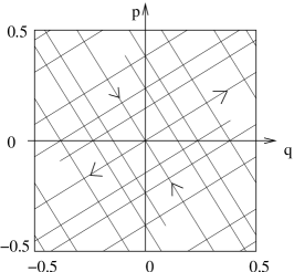
Figure 4: The stable and unstable axes through $0$ of the map $M_{\rm Arnold}$ wrap around the torus at infinity. We have only represented the first six occurrences.

For any hyperbolic matrix $M$, the slopes $s_{+}$ and $s_{-}$ of the unstable and stable directions are quadratic irrationals (i.e. the solutions of a quadratic equation with integer coefficients). It is well known [Kh] that any quadratic irrational $s$ satisfies the following diophantine inequality:

$$\exists C(s)>0,\ \forall k\in\mathbb{Z},\ \forall l\in\mathbb{N}^{*},\quad\left|s-\frac{k}{l}\right|\geq C(s)\frac{1}{l^{2}}\Longleftrightarrow\left|ls-k\right|\geq C(s)\frac{1}{l}.$$

This means that quadratic irrationals are poorly approximated by rationals, in the sense that, to get an approximation with an error $\epsilon$, you need a rational with a denominator of order at least $\epsilon^{-1/2}$.

This inequality will be used in the following manner. Consider the eigenvectors $v_{\pm}$ of $M_{(c,b)}$ defined as $v_{+}=Qe_{q}$ , $v_{-}=Qe_{p}$ (with $Q$ the matrix defined in Eq. (13)). As usual, their dual basis $u_{\pm}$ (defined as $v_{+}\cdot u_{+}=1,\>v_{+}\cdot u_{-}=0$, etc.) can be used to express the coordinates of a point $x$ in the basis $v_{\pm}$:

$$x=q^{\prime}(x)v_{+}+p^{\prime}(x)v_{-},\quad{\rm with}\quad q^{\prime}(x)=x\cdot u_{+},\ \ p^{\prime}(x)=x\cdot u_{-}.$$ (22)

We call d$(x,\mathbb{Z}^{2}_{*})$ the distance between a point $x\in\mathbb{R}^{2}$ and $\mathbb{Z}^{2}_{*}=\mathbb{Z}^{2}\setminus\{0\}$, and we will estimate it for $x$ on the (un)stable axis:

$$\exists C>0,\ \forall x\in\mathbb{R}v_{\pm},\quad{\rm d}(x,\mathbb{Z}^{2}_{*})\geq\frac{C}{\|x\|+1}.$$ (23)

To prove this, first note that, for any $n\in\mathbb{Z}$ s.t. $n_{q}\neq 0$, we have

$$|p^{\prime}(n)|=|n\cdot u_{-}|=|u_{-,p}|\,\left|n_{q}\frac{u_{-,q}}{u_{-,p}}+n_{p}\right|\geq\frac{C(s_{+})|u_{-,p}|}{|n_{q}|},$$ (24)

where we have used the fact that $u_{-,q}/u_{-,p}=s_{+}$ is a quadratic irrational. Interchanging $n_{q}$ and $n_{p}$, we obtain a first set of inequalities:

Lemma 1.

There is a constant $C$ (depending on $M$) such that, for any integer lattice point $n\neq 0$,

$$|p^{\prime}(n)|\geq\frac{C}{\|n\|}\quad\mbox{and}\quad|q^{\prime}(n)|\geq\frac{C}{\|n\|}.$$

We can now prove (23) as follows. For each $x\in\mathbb{R}v_{+}$, there exists an $n\in\mathbb{Z}^{2}_{*}$ so that

$${\rm d}(x,\mathbb{Z}^{2}_{*})=\|n-x\|\geq\frac{|n\cdot u_{-}|}{\|u_{-}\|}\geq\frac{C_{\pm}}{\|u_{-}\|\|n\|}.$$

Since, obviously, $\|n-x\|\leq 1/\sqrt{2}$, (23) follows easily.

We will in addition need a slightly refined statement. If the lattice point $n\neq 0$ is in a sufficiently thin strip around the unstable axis, it satisfies $\|p^{\prime}(n)v_{-}\|\leq 1/2\leq\|n\|/2$, which implies the lower bound $|q^{\prime}(n)|\geq\frac{\|n\|}{2\|v_{+}\|}$. Together with the above lemma, this entails $|p^{\prime}(n)|\geq\frac{C^{\prime}_{1}}{|q^{\prime}(n)|}$ for a certain $C^{\prime}_{1}$. Interchanging $p^{\prime}\leftrightarrow q^{\prime}$, we see that the same inequality holds for points in a sufficiently thin strip around the stable axis. Outside the union of these strips, this inequality can be violated by at most a finite set of lattice points; therefore, upon reducing the constant $C^{\prime}_{1}$ we obtain the main technical result of this section:

Lemma 2.

There exists a constant $C_{o}>0$ (depending on $M$) such that, for any integer points $n\neq m$ of the plane, their coordinates along the (un)stable directions satisfy:

$$|q^{\prime}(n)-q^{\prime}(m)|\geq\frac{C_{o}}{|p^{\prime}(n)-p^{\prime}(m)|}.$$ (25)

These inequalities precisely control the sparseness of the lattice points inside a strip around the unstable axis: the narrower the strip, the farther successive lattice points have to be from each other.

3.2 Quantum mechanics on the torus

We recall as briefly as possible the basic setting for the quantum mechanics of a system with $\mathbb{T}$ as phase space, as well as the quantization of the automorphism $M$, referring to [HB, DE, BouDB] and references therein for further details. In order to define the Hilbert space associated to $\mathbb{T}$, we first consider the translation operators $\hat{T}_{1}=\hat{T}_{(1,0)},\quad\hat{T}_{2}=\hat{T}_{(0,1)}$, which satisfy $\hat{T}_{1}\hat{T}_{2}=\rm e^{-{\rm i}/\hbar}\hat{T}_{2}\hat{T}_{1}$ as a result of (19). So for the values of $\hbar$ defined as:

$$N=\frac{1}{2\pi\hbar}\in\mathbb{N}^{*},$$ (26)

one has the property $\left[\hat{T}_{1},\hat{T}_{2}\right]=0.$ The Hilbert space $L^{2}(\mathbb{R})$ may then be decomposed as a direct integral of the joint eigenspaces of $\hat{T}_{1}$ and $\hat{T}_{2}$:

$$L^{2}(\mathbb{R})=\int^{\oplus}{\cal H}_{N,\theta}\,\frac{d^{2}\theta}{(2\pi)^{2}},\ \ \ {\cal H}_{N,\theta}=\left\{|\psi\rangle\in{\cal S}^{\prime}(\mathbb{R})\ \big{|}\ \hat{T}_{1}|\psi\rangle=\rm e^{{\rm i}\theta_{1}}|\psi\rangle,\hat{T}_{2}|\psi\rangle=\rm e^{{\rm i}\theta_{2}}|\psi\rangle\right\}.$$ (27)

The ‘angle’ $\theta=(\theta_{1},\theta_{2})\in[0,2\pi[^{2}$ thus describes the periodicity properties of the wave function under translations by an elementary cell. $\mathcal{H}_{N,\theta}$ is $N$-dimensional.

We can define a projector $\hat{P}_{\theta}$ from ${\cal S}(\mathbb{R})$ onto the space $\mathcal{H}_{N,\theta}$:

$$\hat{P}_{\theta}=\sum_{(n_{1},n_{2})\in\mathbb{Z}^{2}}\rm e^{-{\rm i}n_{1}\theta_{1}-{\rm i}n_{2}\theta_{2}}\>\hat{T}_{1}^{n_{1}}\>\hat{T}_{2}^{n_{2}}=\sum_{n\in\mathbb{Z}^{2}}\rm e^{-{\rm i}\theta\cdot n+{\rm i}\delta_{n}}\>\hat{T}_{n}.$$ (28)

The phase $\delta_{n}=-n_{1}n_{2}N\pi$ comes from the decomposition $\hat{T}_{n}=\rm e^{-{\rm i}\delta_{n}}\,\hat{T}_{1}^{n_{1}}\hat{T}_{2}^{n_{2}}$.

The Weyl quantization of a function $f(x)=\sum_{k\in\mathbb{Z}^{2}}f_{k}\rm e^{2{\rm i}\pi(x\wedge k)}$ is an operator on $\mathcal{H}_{N,\theta}$ defined by

$$\hat{f}=\sum_{k\in\mathbb{Z}^{2}}f_{k}\>\hat{T}_{k/N}.$$ (29)

For $|\psi\rangle\in\mathcal{H}_{N,\theta}$, its “Wigner function” $W_{\psi}(x)$ is the distribution implicitly defined via

$$\langle\psi|\hat{f}|\psi\rangle=\int_{\mathbb{T}}f(x)\ W_{\psi}(x)\ dx,\ \ \mbox{ so that }\ \tilde{W}_{\psi}(k)=\langle\psi|\hat{T}_{k/N}|\psi\rangle$$ (30)

where the $\tilde{W}_{\psi}(k)=\int_{\mathbb{T}}\rm e^{2{\rm i}\pi(x\wedge k)}\;W_{\psi}(x)\,dx$ are the Fourier coefficients of $W_{\psi}$.

Let now $M\in{\rm SL}(2,\mathbb{Z})$, so that $A,B,C,D$ (see Eq. (10)) are integers. One then easily deduces from (20) and (28) that the quantum map $\hat{M}$ satisfies:

$$\hat{M}\,\hat{P}_{\theta}=\hat{P}_{\theta^{\prime}}\,\hat{M},\quad\mbox{with}\quad\theta^{\prime}=\theta M^{-1}+2\pi\frac{N}{2}\left(CD,AB\right).$$ (31)

The constant shift on the right hand side (RHS) is due to the phases $\delta_{n}$ appearing in (28). $\hat{M}$ will define an endomorphism in $\mathcal{H}_{N,\theta}$ provided $\theta^{\prime}\equiv\theta\bmod 2\pi$, i.e. provided $\theta$ is a fixed point of the dual map defined in (31). Given a hyperbolic matrix $M$, such a fixed point exists for any $N$ [DE]. In particular, for any matrix $M$ the angle $\theta=(0,0)$ (periodic wavefunctions) is a fixed point if $N$ is even, while $\theta=(\pi,\pi)$ (antiperiodic wave wavefunctions) is a fixed point for $N$ odd. We will always make this choice for our numerical examples.

From now on, we will assume that $M=\pm M_{(c,b)}\in{\rm SL}(2,\mathbb{Z})$ is a fixed hyperbolic matrix defining a dynamics on the plane and on the torus. We will therefore no longer indicate its dependence on $(c,b)$. We will also assume that $\hbar$ is such that (26) holds, and for this $\hbar$ we select an angle such that $\theta^{\prime}\equiv\theta$. In general, $\theta$ can depend on $\hbar$, but we will not indicate this dependence.

4 Coherent states and their evolution

4.1 Standard and squeezed coherent states

With the normalized state $|0\rangle$ defined by $a|0\rangle=0$, a “standard” coherent state is

$$|x\rangle=\hat{T}_{x}|0\rangle,\quad x=(q,p)\in\mathbb{R}^{2}.$$ (32)

More generally, we define for each $\tilde{c}\in\mathbb{C}^{*}$ the “squeezed” coherent states $|x,\tilde{c}\rangle$ by

$$|\tilde{c}\rangle=|0,\tilde{c}\rangle=\hat{M}_{(\tilde{c},0)}|0\rangle,\quad|x,\tilde{c}\rangle=\hat{T}_{x}|\tilde{c}\rangle,$$ (33)

where the “squeezing operator” $\hat{{M}}_{(\tilde{c},0)}$ is defined by (17), with $\tilde{b}=0$. Note that, in view of (15), given $M\in\mathrm{SL}(2,\mathbb{R}),\exists!\tilde{c}\in\mathbb{C},\sigma\in[0,2\pi[$ such that

$$\hat{M}|0\rangle=\rm e^{{\rm i}\sigma}|\tilde{c}\rangle.$$ (34)

For more details on coherent states, we refer to [Z, Pe].

To avoid confusion, we will use a tilde for the parameters of the squeezing operator $\hat{{M}}_{(\tilde{c},0)}$, and keep untilde notations for the parameters of the dynamics defined by the matrix $M\stackrel{{\scriptstyle\rm def}}{{=}}\pm M_{(c,b)}$ that are at any rate kept fixed throughout the further discussion. In the $L^{2}(\mathbb{R})$ representation, the state $|x,\tilde{c}\rangle$ is a Gaussian wave packet with mean position $q$. Its Fourier transform is centered around the mean momentum $p$. For any state $|\psi\rangle\in L^{2}\left(\mathbb{R}\right)$, we define its Bargmann function as $x\mapsto\langle x,\tilde{c}|\psi\rangle$, and its Husimi function to be the positive function $\mathcal{H}_{\tilde{c},\psi}$ defined on phase space $\mathbb{R}^{2}$ by:

$$\mathcal{H}_{\tilde{c},\psi}\left(x\right)=\frac{\left|\langle x,\tilde{c}|\psi\rangle\right|^{2}}{2\pi\hbar},\quad\textrm{which satisfies}\quad\int_{\mathbb{R}^{2}}\mathcal{H}_{\tilde{c},\psi}\left(x\right)dx=\|\psi\|^{2}_{L^{2}(\mathbb{R})}.$$ (35)

Note that for given $|\psi\rangle$, the Bargmann and Husimi functions depend on the choice of $\tilde{c}$. Also, the function $x\mapsto\langle x,\tilde{c}|\psi\rangle$ is the product of a Gaussian factor with a function holomorphic with respect to a $\tilde{c}$-dependent holomorphic structure. The term Bargmann function is usually reserved for the holomorphic factor, but we find it convenient to adopt here a slightly different convention.

We will need the explicit expression of the (standard) Bargmann and Husimi functions of the squeezed coherent state $|\tilde{c}\rangle$:

$$\langle x,0|\tilde{c}\rangle=\frac{1}{\sqrt{\cosh|\tilde{c}|}}\exp\left\{-{\rm i}\frac{\tilde{q}\tilde{p}\tanh|\tilde{c}|}{2\hbar}\right\}\exp\left\{-\frac{1}{2}\left(\frac{\tilde{q}^{2}}{\Delta\tilde{q}^{2}}+\frac{\tilde{p}^{2}}{\Delta\tilde{p}^{2}}\right)\right\}.$$ (36)

Here the unstable-stable frame $(\tilde{q},\tilde{p})$ of the symmetric matrix $M_{(\tilde{c},0)}$ is easily seen from the formulas in Section  2 to be obtained from $(q,p)$ by a rotation of angle $\tilde{\psi}_{+}$ (Figure 5), and the widths are given by

$$\Delta\tilde{q}^{2}=\frac{2\hbar}{\left(1-\tanh\left|\tilde{c}\right|\right)},\quad\Delta\tilde{p}^{2}=\frac{2\hbar}{\left(1+\tanh\left|\tilde{c}\right|\right)}.$$ (37)

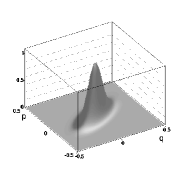
Figure 5: Modulus square of the Bargmann function of a squeezed coherent state $|\tilde{c}\rangle$, as given in (36). The inverse Planck’s constant $N=1/h=40$, and the squeezing parameter $\tilde{c}=-{\rm i}|\tilde{c}|\rm e^{-2{\rm i}\tilde{\psi}_{+}}$ with $|\tilde{c}|=0.962$, $\tilde{\psi}_{+}=32^{\circ}$ (this corresponds to $\tilde{c}_{1}$ for the map $\hat{M}_{\rm Arnold}$). (a) Three dimensional picture. (b) Typical size and orientation of the distribution: ellipse “supporting” the distribution.

Standard and squeezed coherent states on the torus are defined to be the images of the previous coherent states by the projector $\hat{P}_{\theta}$. We use the notation:

$$|x,\tilde{c},\theta\rangle=\hat{P}_{\theta}|x,\tilde{c}\rangle\in{\mathcal{H}}_{N,\theta}.$$ (38)

These states are asymptotically normalized:

$$\langle x,\tilde{c},\theta|x,\tilde{c},\theta\rangle=1+\mathcal{O}(\rm e^{-C(\tilde{c})/\hbar})$$

and satisfy a resolution of the identity on the Hilbert spaces ${\cal H}_{N,\theta}$ [BouDB]:

$$\int_{\mathbb{T}}\frac{dqdp}{2\pi\hbar}\ |x,\tilde{c},\theta\rangle\langle x,\tilde{c},\theta|=\hat{I}_{{\cal H}_{N,\theta}}.$$ (39)

Similarly as above, one defines for any $|\psi\rangle\in{\mathcal{H}}_{N,\theta}$ its Bargmann “function” $x\mapsto\langle x,\tilde{c},\theta|\psi\rangle$ (which is actually a section of a suitable line bundle over $\mathbb{T}$, i.e. a quasiperiodic function on $\mathbb{R}^{2}$, but this shall not interest us here), and Husimi function $\mathcal{H}_{\tilde{c},\psi,\theta}(x)=N\left|\langle x,\tilde{c},\theta|\psi\rangle\right|^{2},$ a bona fide function on the torus (of which we omit to indicate the $N$-dependence).

4.2 The evolution of coherent states

Before turning to quasimodes, we need to study in detail the quantum evolution of the squeezed coherent state $|\tilde{c},\theta\rangle$ which is given by $|t;\tilde{c},\theta\rangle\stackrel{{\scriptstyle\rm def}}{{=}}\hat{M}^{t}|\tilde{c},\theta\rangle$, $t\in\mathbb{Z}$. We will extend this notation to any real time, by $|t;\tilde{c},\theta\rangle\stackrel{{\scriptstyle\rm def}}{{=}}\hat{P}_{\theta}\rm e^{-{\rm i}\hat{H}t/\hbar}|\tilde{c}\rangle$. Due to (34), the states $|t;\tilde{c},\theta\rangle$ are again squeezed coherent states (up to a global phase), so this evolution defines a time flow $\tilde{c}(t)$ on the family of squeezed coherent states centered at the origin. All squeezed states at the origin have even parity: $\hat{P}|\tilde{c}\rangle=|\tilde{c}\rangle$, so that the evolution of $|\tilde{c}\rangle$ through the map $\hat{M}\hat{P}$ is the same as through $\hat{M}$ (yet, these two maps might require different values for $\theta$, see Eq. (31)).

It will turn out that $|t;\tilde{c},\theta\rangle$ will be most simply described if the initial squeezed state $|\tilde{c}_{0},\theta\rangle$ at time $t=0$ is well chosen in terms of the decomposition (13). Defining, with the notations of (13)–(14), $\tilde{c}_{0}=-b_{2}\rm e^{-2{\rm i}b_{1}}$, it is easy to check that $|\tilde{c}_{0}\rangle=\rm e^{-{\rm i}b_{1}/2}\hat{Q}|0\rangle$ since $\hat{M}_{(\tilde{c}_{0},0)}=\hat{R}(b_{1})\hat{B}(b_{2})\hat{R}(-b_{1})$ and $\hat{R}(-b_{1})|0\rangle=\rm e^{-{\rm i}b_{1}/2}|0\rangle$. Then, with $\hat{M}=\hat{Q}\hat{D}(\lambda)\hat{Q}^{-1}$,

$$\hat{M}^{t}|\tilde{c}_{0}\rangle=\rm e^{-{\rm i}b_{1}/2}\hat{Q}\,\hat{D}(\lambda t)|0\rangle,\qquad\langle\tilde{c}_{0}|\hat{M}^{t}|\tilde{c}_{0}\rangle=\langle 0|\hat{D}(\lambda t)|0\rangle=\frac{1}{\sqrt{\cosh(\lambda t)}}\in\mathbb{R}^{+},$$ (40)

so the overlap $\langle\tilde{c}_{0}|\hat{M}^{t}|\tilde{c}_{0}\rangle$ is real positive for all times.

For later purposes we note that, defining, for $s\in\mathbb{R}$, $\tilde{c}_{s}\in\mathbb{C},\sigma_{s}\in[0,2\pi[$ by

$$\rm e^{-{\rm i}\frac{\hat{H}}{\hbar}s}|\tilde{c}_{0}\rangle=\rm e^{{\rm i}\sigma_{s}}|\tilde{c}_{s}\rangle,$$ (41)

(see (34)), it is clear that $\langle\tilde{c}_{s}|\rm e^{-{\rm i}\hat{H}t/\hbar}|\tilde{c}_{s}\rangle$ is real positive for all $t$. In fact, it can be shown that the $\tilde{c}_{s}$ are the only values of $\tilde{c}$ with this property. Among all $s$, $s=0$ maximizes $\left|\langle 0|\tilde{c}_{s}\rangle\right|^{2}$, so $|\tilde{c}_{0}\rangle$ is in a sense the most localized state among all $|\tilde{c}_{s}\rangle$.

In this paper, we will almost exclusively build quasimodes from coherent states with “squeezing” $\tilde{c}_{0}$; this choice is made for pure convenience, and our main semiclassical results apply to more general squeezings as well (see Section 6.6 and Appendix 10.2).

Before turning to $|t;\tilde{c},\theta\rangle\in{\cal H}_{N,\theta}$, we first describe the evolved state $|t;\tilde{c}_{0}\rangle\stackrel{{\scriptstyle\rm def}}{{=}}\rm e^{-{\rm i}\hat{H}t/\hbar}|\tilde{c}_{0}\rangle\in L^{2}(\mathbb{R})$, by studying its Husimi function on the plane, as defined in (35). It will be convenient (but again not absolutely necessary for our results, see Section 10.2) to adapt the choice of $\tilde{c}$ in the definition of this Husimi function to the dynamics $M$ by putting $\tilde{c}=\tilde{c}_{0}$. One then computes

$${\mathcal{H}}_{\tilde{c}_{0},t}(x)\stackrel{{\scriptstyle\rm def}}{{=}}\frac{\left|\langle\tilde{c}_{0}|\hat{T}^{\dagger}_{x}|t;\tilde{c}_{0}\rangle\right|^{2}}{2\pi\hbar}=\frac{\left|\langle 0|\hat{Q}^{\dagger}\hat{T}^{\dagger}_{x}\hat{Q}\hat{D}\left(\lambda t\right)\hat{Q}^{\dagger}\hat{Q}|0\rangle\right|^{2}}{2\pi\hbar}=\frac{\left|\langle 0|\hat{T}^{\dagger}_{Q^{-1}x}\hat{D}\left(\lambda t\right)|0\rangle\right|^{2}}{2\pi\hbar}.$$ (42)

It is now natural to use the coordinates $\left(q^{\prime},p^{\prime}\right)=Q^{-1}\left(q,p\right)\in\mathbb{R}^{2}$ attached to the unstable-stable basis $({v}_{+,\,}{v}_{-})$ (see Eq. (22)). In terms of these, the Husimi function is a Gaussian drawn on the unstable and stable axes:

$$\mathcal{H}_{\tilde{c}_{0},t}(x)=\frac{1}{2\pi\hbar\cosh(\lambda t)}\exp\left(-\frac{q^{\prime 2}}{\Delta q^{\prime 2}}-\frac{p^{\prime 2}}{\Delta p^{\prime 2}}\right),$$ (43)

with

$$\Delta q^{\prime 2}=\frac{2\hbar}{1-\tanh(\lambda t)}\stackrel{{\scriptstyle t\to\infty}}{{\sim}}\hbar\,\rm e^{2\lambda t},\qquad\Delta p^{\prime 2}=\frac{2\hbar}{1+\tanh(\lambda t)}=\rm e^{-2\lambda t}\Delta q^{\prime 2}\stackrel{{\scriptstyle t\to\infty}}{{\rightarrow}}\hbar.$$ (44)

The Husimi distribution of the evolved state $|t;\tilde{c}_{0}\rangle$ therefore spreads exponentially (with rate $\lambda$) in the unstable direction of the map, and has a finite transverse width $\sqrt{\hbar}$. It “lives” in an elliptic region of phase space centered on the origin and of area $\Delta q^{\prime}\Delta p^{\prime}\sim\hbar\rm e^{\lambda t}$. Due to conservation of the total probability, the height of the distribution decreases exponentially.

We now turn to $|t;\tilde{c}_{0},\theta\rangle=\hat{M}^{t}|\tilde{c}_{0},\theta\rangle$, $t\geq 0$ and its Husimi function

$${\mathcal{H}}_{\tilde{c}_{0},t,\theta}(x)=N|\langle x,\tilde{c}_{0}|\hat{P}_{\theta}|t;\tilde{c}_{0}\rangle|^{2}.$$

It is clear from (28) that $\langle x,\tilde{c}_{0}|\hat{P}_{\theta}|t;\tilde{c}_{0}\rangle$ is obtained by summing (up to some phases) the translates of the function $\langle x,\tilde{c}_{0}|t;\tilde{c}_{0}\rangle$ into the different phase space cells of size $1$ centered on the points of $\mathbb{Z}^{2}$ (the cell around $0$ will be called the fundamental cell $\mathcal{F}$). Consequently, it follows from (43)–(44) that this function is non-negligible at a point $x\in\mathcal{F}$ only if $x$ lies within a distance $\sqrt{\hbar}$ from a stretch of length $\Delta q^{\prime}\approx\sqrt{\hbar}\rm e^{\lambda t}=\rm e^{\lambda(t-T/2)}$ of the unstable manifold through $0$ (Figure 6). Here we introduced the Ehrenfest time as

$$T\stackrel{{\scriptstyle\rm def}}{{=}}\frac{|\log\hbar|}{\lambda}.$$ (45)

Since at time $|\log\hbar|/(2\lambda)=T/2$, $\Delta q^{\prime}$ reaches the size $1$ (i.e. the size of the torus), it is clear that for shorter times the Husimi function ${\mathcal{H}}_{\tilde{c}_{0},t,\theta}$ lives in an elliptic region of shrinking diameter $\sqrt{\hbar}\rm e^{\lambda t}$ around $0$.

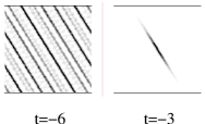
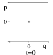
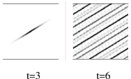
Figure 6: Husimi function of the state $|t;\tilde{c}_{0},\theta\rangle$ for the dynamics (21) and $N=1/(2\pi\hbar)=500$. One has $T\approx 8.37$.

For times larger than $T/2$, this Husimi function starts to wrap itself around the torus along the unstable axis or, equivalently, the support of some of the translates $\langle x+n,\tilde{c}_{0}|t;\tilde{c}_{0}\rangle$ start to enter into the fundamental cell. The diophantine properties guarantee that the branches of the piece of length $\Delta q^{\prime}$ of the unstable manifold passing through the origin are roughly at a distance $1/\Delta q^{\prime}=\rm e^{-\lambda(t-T/2)}$ from each other (Fig.  4). Consequently, as long as $\Delta p^{\prime}<<\rm e^{-\lambda(t-T/2)}$, i.e. as long as $t\leq(1-\epsilon)T$, the main contribution to $\langle x,\tilde{c}_{0}|\hat{P}_{\theta}|t;\tilde{c}_{0}\rangle$ and hence to the Husimi function $\mathcal{H}_{\tilde{c}_{0},t,\theta}$ comes from a single term $\langle x+n,\tilde{c}_{0}|t;\tilde{c}_{0}\rangle$ for most $x\in\mathcal{F}$. We say there are no interference effects. The regime $(1+\epsilon)T/2\leq t\leq(1-\epsilon)T$ was studied in [BonDB1] where it was proven that on that time scale the Husimi function equidistributes on the torus.

For longer times $t\geq(1+\epsilon)T$, when the area $\Delta p^{\prime}\Delta q^{\prime}$ occupied by the support of $\mathcal{H}_{\tilde{c}_{0},t}$ becomes larger than the area of the torus itself, several terms may contribute equally to $\langle x,\tilde{c}_{0}|\hat{P}_{\theta}|t;\tilde{c}_{0}\rangle$. In the next subsection we give a detailed control on the onset of this “interference regime” up to time $2T$ for the Husimi function of $|t;\tilde{c}_{0},\theta\rangle$ evaluated at the origin $x=0$; we shall show that the interferences remain “small” up to the time $2T$.

As a last remark, we point out that the above discussion is symmetric with respect to time reversal. For negative times, $\mathcal{H}_{\tilde{c}_{0},t,\theta}$ spreads along the stable direction, reaches the boundary of $\mathcal{F}$ around $-T/2$, and will interfere with itself for $t\leq-T$.

4.3 Estimating the interference effects

As explained in the introduction, our crucial technical estimate concerns the autocorrelation function for the state $|\tilde{c}_{0},\theta\rangle$, given by $\langle\tilde{c}_{0},\theta|\hat{M}^{t}|\tilde{c}_{0},\theta\rangle$. More generally, we will need control on

$$\langle\tilde{c}_{s},\theta|\hat{M}^{t}|\tilde{c}_{s},\theta\rangle=\langle\tilde{c}_{s}|\hat{P}_{\theta}\hat{M}^{t}|\tilde{c}_{s}\rangle=\langle\tilde{c}_{s}|\hat{M}^{t}|\tilde{c}_{s}\rangle+I(t,s),$$ (46)

where we separated the contribution of the term $n=(0,0)$ (the “plane overlap”), from the remaining terms:

$$I(t,s)\stackrel{{\scriptstyle\rm def}}{{=}}\sum_{n\in\mathbb{Z}^{2}_{*}}\rm e^{-{\rm i}n\cdot\theta+{\rm i}\delta_{n}}\>\langle\tilde{c}_{s}|\hat{T}_{n}\,\hat{M}^{t}|\tilde{c}_{s}\rangle.$$ (47)

This remainder represents the interference of the evolved plane coherent state with the lattice-translated initial state. We will show that these contributions tend to $0$ as $N\to\infty$, uniformly for all times $|t|\leq 2(1-\epsilon)T$, for any fixed $\epsilon>0$.

A trivial upper bound is

$$\left|I(t,s)\right|\leq\sum_{n\in\mathbb{Z}^{2}_{*}}\left|\langle n,\tilde{c}_{s}|\rm e^{-\frac{i}{\hbar}\hat{H}t}|\tilde{c}_{s}\rangle\right|\stackrel{{\scriptstyle\rm def}}{{=}}J_{0}(t,s),$$ (48)

and we shall estimate the RHS. Note that we extended $I(t,s)$ in the natural way to real times $t$. The detailed proofs of the estimates below are given in Appendix 10.1; here we limit ourselves to explaining the underlying ideas and to an instructive comparison with a numerical example. For simplicity, we will concentrate on the case $s=0$.

We define a time-dependent metric on the plane adapted to the Gaussian in (43):

$$\|\,x\,\|^{2}_{t}\ \stackrel{{\scriptstyle\rm def}}{{=}}\ \frac{1}{2}\left(\frac{q^{\prime}(x)}{\Delta q^{\prime}(t)}\right)^{2}+\frac{1}{2}\left(\frac{p^{\prime}(x)}{\Delta p^{\prime}(t)}\right)^{2}.$$

The RHS of (48) is simply the sum of this Gaussian of height $H_{t}=(\cosh\lambda t)^{-1/2}$ evaluated at all nonzero integer lattice points. The diophantine properties proven in Section  3.1 provide information on the position of the integer lattice with respect to the ellipse $\{\|x\|^{2}_{t}=\nolinebreak 1\}$ and allow us to prove the following estimates:

• for relatively short times (meaning $|t|\leq(1-\epsilon)T$), all lattice points $n\neq 0$ are far outside the support of the Gaussian so that $\|n\|_{t}$ is large. In fact, the distance $\|n\|_{t}$ reaches its minimum for a single point $n_{o}$ (more precisely a finite number $\mathcal{N}$ of points), with $\|n_{o}\|^{2}_{t}>c\,\frac{\rm e^{-\lambda|t|}}{\hbar}>>1$. Note that, here and in the following, we write $f(\hbar)<<g(\hbar)$ when $\lim_{\hbar\to 0}f(\hbar)/g(\hbar)=0$. $J_{0}(t,0)$ is dominated by the contribution of this finite set of points, given by $\mathcal{N}\,H_{t}\exp\left\{-\|n_{o}\|^{2}_{t}\right\}$, the contributions of farther points being much smaller. The precise bound proven in the appendix reads:

  $$|t|\leq T\Longrightarrow|I(t,0)|\leq 2\sqrt{2}\,\rm e^{-\lambda|t|/2}\,\exp\left\{-C_{o}\frac{\rm e^{-\lambda|t|}}{2\hbar}\right\}\left[1+C\rm e^{\lambda(|t|-T)/2}\right],$$ (49)

  where the constant $C_{o}$ is the parameter of the diophantine equation (25), and $C$ can be computed explicitly (it depends only on $M$).

• For times $|t|\geq T$, a large number of lattice points ($\mathcal{N}_{t}=\Delta q^{\prime}(t)\Delta p^{\prime}(t)\sim\rm e^{\lambda(|t|-T)}$) are contained in the ellipse (i.e. satisfy $\|n\|_{t}\leq 1$), and their collective contribution dominates the RHS of (48): $|I(t)|\lesssim\mathcal{N}_{t}H_{t}\sim\rm e^{\lambda(-T+|t|/2)}$. This is indeed essentially what we prove:

  $$T\leq|t|\Longrightarrow|I(t,0)|\leq\frac{2\pi\sqrt{2}}{C_{o}}\,\rm e^{\lambda(-T+|t|/2)}\,\left[1+C^{\prime}\rm e^{\lambda(T-|t|)/2}\right],$$ (50)

  where $C^{\prime}$ can be computed explicitly in terms of $M$. This upper bound becomes of order unity for $|t|\simeq 2T$.

• From the definition (46), we have trivially for any time

  $$|I(t,0)|\leq\langle\tilde{c}_{0},\theta|\tilde{c}_{0},\theta\rangle+\langle\tilde{c}_{0}|\hat{M}^{t}|\tilde{c}_{0}\rangle\leq 1+\mathcal{O}\left(\rm e^{-C(\tilde{c}_{0})/\hbar}\right)+\frac{1}{\sqrt{\cosh(\lambda|t|)}}.$$

Combining these estimates (generalized to $s\neq 0$), one obtains the following proposition:

Proposition 1.

There exist positive constants $C$, $C^{\prime}$, $C^{\prime\prime}$ such that for all times $t\in\mathbb{R}$, and for all $s$ in a bounded interval

$$|I(t,s)|\leq J_{0}(t,s)\leq\min\left(C\hbar\rm e^{\lambda|t|/2},\>1+\sqrt{2}\rm e^{-\lambda|t|/2}+C^{\prime}\rm e^{-C^{\prime\prime}/\hbar}\right).$$ (51)

This shows that the interferences remain small until times of order $2T$. The existence of “short quantum periods” for certain values of $\hbar$ (see the introduction and Section 8) implies that $I(t,0)$ is of order $1$ at $t=P\simeq 2T$ for these values of $\hbar$. This is further illustrated in Figure 7.

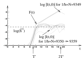
Figure 7: Numerical calculations of $\log|I(t,0)|$, for the map (21). The heuristic upper bound $F(t)$ (solid line) is defined in terms of the shifted Ehrenfest time $T^{\prime}=\log(N)/\lambda$: $F(t)=-\frac{\lambda t}{2}-\rm e^{\lambda\left(T^{\prime}-t\right)}-1$ for $0<t<T^{\prime}$ and $F(t)=\frac{\lambda}{2}\left(t-2T^{\prime}\right)+0.5$ for $T^{\prime}<t<2T^{\prime}$. The horizontal dashed line at $\log(h^{1/2})$ gives the order of magnitude of the plateau for $t>T^{\prime}$.

Figure 7 shows numerical calculations of $\log|I(t,0)|$ for values of Planck’s “constant” $N=9349\rightarrow 9359$ and compares them to $F(t)$, which is essentially given by the upper bounds (49)–(50). We observe that, whereas (49) is close to optimal, the same is not true for (50) for most values of $N$: there is a “plateau” $\log|I(t,0)|\simeq\log(\hbar^{1/2})$ for $t>T^{\prime}$, where $T^{\prime}=\log(N)/\lambda$ is a shifted Ehrenfest time. This plateau can be explained by assuming that the phases which multiply the different terms in $I(t,0)$ are uncorrelated, like independent random phases. For $t>>T$, the RHS of (47) could then be replaced by a sum of many ($\simeq\mathcal{N}_{t}$) terms with identical moduli $H_{t}$ but random uncorrelated phases, similar to a 2-dimensional random walk. The modulus of the sum (i.e. the length of the random walk) has a typical value $|I(t,0)|\sim\sqrt{\mathcal{N}_{t}}\,H_{t}\sim\hbar^{1/2}$, independent of time: this is indeed what we see numerically.

However, for the value of $N=9349$, corresponding to a “short quantum period” $P=19$, as discussed in Section 8, $\log|I(t,0)|$ is close to the upper bounds (49)–(50) up to time $P\simeq 2T^{\prime}$. In such exceptional cases —crucial in this paper— there appears strong correlations between the phases in the sum $I(t,0)$: the random walk somehow becomes “rigid”, which makes its total length of the same order as the sum of individual lengths, $|I(t,0)|\sim J_{0}(t,0)\sim\mathcal{N}_{t}H_{t}$. This rigidity can actually by analyzed directly from the explicit expression for the phases [FN2]: one first finds that for these special values of Planck’s constant $N=N_{k}$ and $t$ in the interval $T<t<2T$, the phases corresponding to the relevant $\sim\mathcal{N}_{t}$ lattice points are all close to $2d$-th roots of unity, where $d=({\rm tr}M)^{2}-4$ (in the example $M=M_{\rm Arnold}$ and $N_{k}=9349$, the relevant phases are all close to unity). Then, the sum of these $\sim\mathcal{N}_{t}$ phases behaves like $G(M,N_{k})\mathcal{N}_{t}$ for $\mathcal{N}_{t}>>1$, and one can check that the prefactor $G(M,N_{k})$ (a Gauss sum) is bounded away from zero uniformly (e.g. $G(M_{\rm Arnold},9349)=1$). This explains the behaviour $|I(t,0)|\sim J_{0}(t,0)$. This situation drastically differs from the case of a “generic” $N$, where the relevant phases are more or less equidistributed over the circle.

5 Quasimodes at the origin

5.1 Continuous time versus discrete time quasimodes

We are now ready to study the quasimodes (2) and (6) “associated” with the periodic orbits of the dynamics generated by $M$, as discussed in the introduction. To alleviate the notations, we start with the case where the orbit is simply the fixed point $(0,0)\in\mathbb{T}$. The rather straightforward generalization to arbitrary orbits is given in Section 7. Note that the Ehrenfest time $T=\frac{|\ln\hbar|}{\lambda}$ is in general not an integer: whenever $T$ or $T/2$ appears in a sum boundary, they should therefore be replaced by the nearest integer.

It will be convenient to also consider slightly modified quasimodes, for which the initial state is not the squeezed coherent state $|\tilde{c}_{0},\theta\rangle$ as in (2), but rather the following superposition of squeezed coherent states:

$$\hat{P}_{\theta}\>\int^{1}_{0}dt\,\rm e^{-{\rm i}\phi t}\rm e^{-\frac{{\rm i}}{\hbar}\hat{H}t}|\tilde{c}_{0}\rangle.$$ (52)

The “continuous time” version of the quasimodes defined in (2) then reads:

$$|\Phi^{\rm cont}_{\phi}\rangle \stackrel{{\scriptstyle\rm def}}{{=}}\hat{\mathcal{P}}_{-T,T,\phi}\>\hat{P}_{\theta}\>\int^{1}_{0}dt\,\rm e^{-{\rm i}\phi t}\rm e^{-\frac{{\rm i}}{\hbar}\hat{H}t}|\tilde{c}_{0}\rangle$$ (53)

$$=\hat{P}_{\theta}\>\int_{-T}^{T}dt\,\rm e^{-{\rm i}\phi t}\rm e^{-\frac{{\rm i}}{\hbar}\hat{H}t}|\tilde{c}_{0}\rangle.$$ (54)

Here we introduced, for any $\phi\in\mathbb{R},t_{0}<t_{1}\in\mathbb{Z}$, the operator

$$\hat{\mathcal{P}}_{t_{0},t_{1},\phi}=\sum_{t=t_{0}}^{t_{1}-1}\rm e^{-{\rm i}t\phi}\hat{M}^{t},$$ (55)

and the equality (54) follows from a trivial computation.

These quasimodes can also be decomposed into 4 parts $|\Phi^{\rm cont}_{j,\phi}\rangle$, obtained by integrating in $t$ over time intervals of length $T/2$, then projecting the obtained state in ${\cal H}_{N,\theta}$. A remarkable and useful property (derived from Poisson’s formula) is that we can recover the “discrete time” quasimodes $|\Phi^{\rm disc}_{\phi}\rangle$ defined in (2) from the “continuous time” ones:

$$|\Phi^{\rm disc}_{\phi}\rangle=\sum_{k\in\mathbb{Z}}|\Phi^{\rm cont}_{\phi+2\pi k}\rangle.$$

Notice that the state in (52) is not $2\pi$-periodic with respect to $\phi$ so that the quasimodes $|\Phi^{\rm cont}_{\phi}\rangle$ depend on the “quasienergy” $\phi\in\mathbb{R}$.

The main reason for considering continuous time quasimodes is that they are easily connected with generalized eigenstates of the Hamiltonian $\hat{H}$, which allows to pointwise describe their Husimi densities, a task we turn to in Section 6.

In the next subsection, we start our study of the above quasimodes. We will use from now on the notation $|\Phi_{\phi}\rangle$ in statements that are valid both for $|\Phi^{\rm disc}_{\phi}\rangle$ and $|\Phi^{\rm cont}_{\phi}\rangle$ (and similarly for $|\Phi_{j,\phi}\rangle$).

5.2 Orthogonality of the states $|\Phi_{j,\phi}\rangle_{n}$ at fixed $\phi$

Proposition 2.

(i) The states $|\Phi_{j,\phi}\rangle$, $j=1,2,3,4$ and $|\Phi_{\phi}\rangle$ satisfy, as $\hbar\to 0$

$$\langle\Phi_{j,\phi}|\Phi_{j,\phi}\rangle=\frac{T}{2}S_{1}(\lambda,\phi)+\mathcal{O}(1),\qquad\langle\Phi_{\phi}|\Phi_{\phi}\rangle=2TS_{1}(\lambda,\phi)+\mathcal{O}(1),$$ (56)

where the smooth function $S_{1}(\lambda,\phi)$ is strictly positive for all $\phi\in\mathbb{R}$ and $\mathcal{O}(1)$ is uniformly bounded in $\phi$. In particular these states do not vanish for small enough $\hbar$ and the normalized quasimodes $|\Phi_{\phi}\rangle_{n}$ satisfy (5).

(ii) Furthermore, for all $\phi\in\mathbb{R}$, the $|\Phi_{j,\phi}\rangle_{n}$ become mutually orthogonal in the semiclassical limit: for all $j\not=k\in\{1,\ldots,4\}$

$$\lim_{\hbar\to 0}\ {}_{n}\!\langle\Phi_{j,\phi}|\Phi_{k,\phi}\rangle_{n}=0.$$ (57)

The limit is uniform for all $\phi$ in a bounded interval.

(iii) Consequently, for all $\phi\in\mathbb{R}$,

$${}_{n}\!\langle\Phi_{\phi}|\Phi_{j,\phi}\rangle_{n}\rightarrow 1/2,\quad_{n}\!\langle\Phi_{\phi}|\Phi_{{\rm erg},\phi}\rangle_{n}\rightarrow 1/\sqrt{2}\quad\textrm{and}\quad_{n}\!\langle\Phi_{\phi}|\Phi_{{\rm loc},\phi}\rangle_{n}\rightarrow 1/\sqrt{2}.$$

Proof.

(i) We first give a detailed proof for the “continuous time” quasimodes. Writing $k=j-i\in\{0,1,2,3\}$, a simple computation yields (see (41))

$$\langle\Phi_{i,\phi}^{\rm cont}|\Phi_{j,\phi}^{\rm cont}\rangle=\sum_{t=0}^{\frac{T}{2}-1}\sum_{t^{\prime}=0}^{\frac{T}{2}-1}\int_{0}^{1}ds\ \int_{0}^{1}ds^{\prime}\,\rm e^{-{\rm i}(t-t^{\prime}+s-s^{\prime}+kT/2)\phi}\,\langle\tilde{c}_{0}|\hat{P}_{\theta}\rm e^{-\frac{i}{\hbar}\hat{H}(t-t^{\prime}+s-s^{\prime}+kT/2)}|\tilde{c}_{0}\rangle.$$

Using (46) and (48) this becomes:

$$\langle\Phi_{i,\phi}^{\rm cont}|\Phi_{j,\phi}^{\rm cont}\rangle=\int^{T/2}_{-T/2}ds\;\left(\frac{T}{2}-|s|\right)\>\rm e^{-{\rm i}(s+kT/2)\phi}\langle\tilde{c}_{0}|\rm e^{-\frac{i}{\hbar}\hat{H}(s+kT/2)}|\tilde{c}_{0}\rangle+\mathrm{error}$$ (58)

where

$$\mathrm{error}\leq\int_{0}^{1}ds\ \int_{0}^{1}ds^{\prime}\sum_{t=-\frac{T}{2}}^{\frac{T}{2}-1}\big{(}\frac{T}{2}-|s|\big{)}\ J_{0}(t+k\frac{T}{2}+s-s^{\prime},s^{\prime}).$$

Using the bound (51), one readily finds that the second term is $\mathcal{O}(\hbar^{\frac{3-k}{4}})$.

To estimate the norm of $|\Phi_{j}^{\rm cont}\rangle$, there remains to compute the integral in (58) in the case $i=j$, that is $k=0$:

$$\int^{T/2}_{-T/2}ds\;(T/2-|s|)\,\rm e^{-{\rm i}s\phi}\langle\tilde{c}_{0}|\rm e^{-\frac{i}{\hbar}\hat{H}s}|\tilde{c}_{0}\rangle =\int^{T/2}_{-T/2}ds\,\frac{(T/2-|s|)\rm e^{-{\rm i}s\phi}}{\sqrt{\cosh(\lambda s)}}$$

$$=\frac{T}{2}\,S_{1}^{\rm cont}(\lambda,\phi,T/2)-S_{2}^{\rm cont}(\lambda,\phi,T/2),$$

where the (real) functions $S_{1}^{\rm cont}$, $S_{2}^{\rm cont}$ are defined as follows:

$$S_{1}^{\rm cont}(\lambda,\phi,\tau)\stackrel{{\scriptstyle\rm def}}{{=}}\int^{\tau}_{-\tau}dt\,\frac{\rm e^{-{\rm i}t\phi}}{\sqrt{\cosh\left(\lambda t\right)}},\quad S_{2}^{\rm cont}(\lambda,\phi,\tau)\stackrel{{\scriptstyle\rm def}}{{=}}\int^{\tau}_{-\tau}dt\,\frac{\left|t\right|\rm e^{-{\rm i}t\phi}}{\sqrt{\cosh\left(\lambda t\right)}}.$$ (59)

The limits of $S_{i}^{\rm cont}(\lambda,\phi,\tau)$ as $\tau\rightarrow\infty$ clearly exist. We only give the value for $S_{1}^{\rm cont}$, the most relevant one for our purposes [BaTIT]:

$$S_{1}^{\rm cont}(\lambda,\phi)\stackrel{{\scriptstyle\rm def}}{{=}}\lim_{\tau\to\infty}S_{1}^{\rm cont}(\lambda,\phi,\tau)=\frac{1}{\lambda\sqrt{2\pi}}\left|\Gamma\left(\frac{1}{4}+{\rm i}\frac{\phi}{2\lambda}\right)\right|^{2}.$$ (60)

For fixed $\lambda$, this function is maximal for $\phi=0$ (with value $\approx 5.244/\lambda$), and decreases as $\sqrt{\frac{4\pi}{\lambda|\phi|}}\rm e^{-\pi|\phi|/2\lambda}$ for $|\phi|\to\infty$. A crucial property is the strict positivity of this function, for all values $\lambda>0$, $\phi\in\mathbb{R}$.

The computation of $\langle\Phi_{\phi}|\Phi_{\phi}\rangle$ is similar.

(ii) We now estimate the overlaps $\langle\Phi_{i,\phi}|\Phi_{j,\phi}\rangle$ for $j\neq i$, by estimating the first integral of (58) in the cases $3\geq k\geq 1$:

$$\left|\int^{T/2}_{-T/2}ds\;\left(T/2-|s|\right)\frac{\rm e^{-{\rm i}(s+kT/2)\phi}}{\sqrt{\cosh(\lambda(s+kT/2))}}\right|\leq\frac{4\sqrt{2}}{\lambda^{2}}\rm e^{-\frac{\lambda(k-1)T}{4}}=\mathcal{O}(\hbar^{\frac{k-1}{4}}).$$

Taking into account the estimate of the error in (58), we see that for any $i\neq j$, the overlap $\langle\Phi_{i,\phi}^{\rm cont}|\Phi_{j,\phi}^{\rm cont}\rangle$ is bounded by a constant (even by $\mathcal{O}(\hbar^{1/4})$ for $|i-j|=2)$. As a result,

$$\forall i\neq j,\quad_{n}\!\langle\Phi_{i,\phi}^{\rm cont}|\Phi_{j,\phi}^{\rm cont}\rangle_{n}=\frac{\langle\Phi_{i,\phi}^{\rm cont}|\Phi_{j,\phi}^{\rm cont}\rangle}{\langle\Phi_{i,\phi}^{\rm cont}|\Phi_{i,\phi}^{\rm cont}\rangle}\leq\frac{C}{T}.$$ (61)

This proves (ii). Part (iii) is now obvious.

To treat the case of the discrete quasimodes, the integrals over time have to be replaced by sums over integers. For instance, the expressions defined in (59) are replaced by

$$S^{\rm disc}_{1}(\lambda,\phi,\tau)\stackrel{{\scriptstyle\rm def}}{{=}}\sum_{|t|\leq\tau}\frac{\rm e^{-{\rm i}t\phi}}{\sqrt{\cosh\left(\lambda t\right)}},$$

and similarly for $S_{2}$. The sum $S_{1}^{\rm disc}(\lambda,\phi)=\lim_{\tau\to\infty}S^{\rm disc}_{1}(\lambda,\phi,\tau)$ is also nonnegative for all $\lambda>0$, $\phi\in[-\pi,\pi]$. Indeed, Poisson’s formula induces the identity

$$S^{\rm disc}_{1}(\lambda,\phi)=\sum_{k\in\mathbb{Z}}S_{1}^{\rm cont}(\lambda,\phi+2k\pi).$$

The norms of the discrete quasimodes therefore satisfy an estimate similar to (57), upon replacing $S_{1}^{\rm cont}$ by $S_{1}^{\rm disc}$. The other estimates are identical as for the continuous version. ∎

5.3 Quasimodes of different quasienergies

We now compare quasimodes $|\Phi_{\phi}\rangle$ of different quasienergies and show:

Proposition 3.

Let $\phi_{0}$ be an arbitrary angle in $[0,2\pi[$, and

$$\phi_{k}=\phi_{0}+\frac{\pi}{T}k,\quad k=1,\ldots,2T.$$

The $2T$ quasimodes $|\Phi_{\phi_{k}}\rangle_{n}$ become mutually orthogonal in the semiclassical limit: $\forall k^{\prime}\neq k$, ${}_{n}\!\langle\Phi_{\phi_{k^{\prime}}}|\Phi_{\phi_{k}}\rangle_{n}=\mathcal{O}(1/T)$.

This is an immediate consequence of the following finer estimate:

Proposition 4.

Let $I\subset\mathbb{R}$ be a fixed bounded interval. There exists a constant $C>0$ such that, given any semiclassically vanishing function $\theta(\hbar)$ and $n\in\mathbb{Z}^{*}$, if $\phi,\phi^{\prime}\in I$, and if the phase shift $\Delta\phi=\phi^{\prime}-\phi$ satisfies $|\Delta\phi-\frac{n\pi}{T}|\leq\theta(\hbar)\frac{|n|}{T}$, then we have, for small enough $\hbar$, ${}_{n}\!\langle\Phi_{\phi^{\prime}}|\Phi_{\phi}\rangle_{n}\leq C\left(\theta(\hbar)+\frac{1}{T}\right)$.

Proof.

As before, we write the proof for the continuous time quasimodes. The overlap $\langle\Phi_{\phi^{\prime}}^{\rm cont}|\Phi_{\phi}^{\rm cont}\rangle$ is given by an expression similar to (58). Using the estimate (51) for $I(t,s)$, we obtain

$$\langle\Phi^{\rm cont}_{\phi^{\prime}}|\Phi^{\rm cont}_{\phi}\rangle =\int^{T}_{-T}dt\int^{T}_{-T}dt^{\prime}\>\frac{\rm e^{{\rm i}(t^{\prime}\phi^{\prime}-t\phi)}}{\sqrt{\cosh\lambda(t-t^{\prime})}}+\mathcal{O}(1)$$

$$=\int^{2T}_{-2T}ds\>\frac{\rm e^{{\rm i}s\bar{\phi}}}{\sqrt{\cosh(\lambda s)}}\>\frac{\sin\left\{\Delta\phi\left(T-|s|/2\right)\right\}}{\Delta\phi/2}+\mathcal{O}(1)$$

where we introduced $\bar{\phi}\stackrel{{\scriptstyle\rm def}}{{=}}\frac{\phi^{\prime}+\phi}{2}$. This integral is bounded above by $\frac{2S_{1}(\lambda,0)}{|\Delta\phi|}$, so that for a phase difference bounded away from zero (i.e. $|\Delta\phi|\geq c>0$), the scalar product of the normalized states is ${}_{n}\!\langle\Phi_{\phi^{\prime}}|\Phi_{\phi}\rangle_{n}=\mathcal{O}(T^{-1})$. We are however more interested in the case where $\Delta\phi$ is $\hbar$-dependent and semiclassically small: $\Delta\phi\rightarrow 0$. Inserting $|\sin\{\Delta\phi(T-|s|/2)\}-\sin\{\Delta\phi T\}|\leq|s|\Delta\phi/2$ in the integral and using (56), we get for $\hbar\to 0$, $\Delta\phi\to 0$:

$${}_{n}\!\langle\Phi_{\phi^{\prime}}^{\rm cont}|\Phi_{\phi}^{\rm cont}\rangle_{n}=\frac{S^{\rm cont}(\bar{\phi})}{\sqrt{S^{\rm cont}(\phi)S^{\rm cont}(\phi^{\prime})}}\frac{\sin\left(T\Delta\phi\right)}{T\Delta\phi}\,+\mathcal{O}(1/T).$$

The first term can be as large as $1$, for $\Delta\phi<<T^{-1}$. It will also be large for values $\Delta\phi=\frac{\pi(n+1/2)}{T}$ with $n$ an integer, $|n|<<T$, where it takes the value $\pm 1/T\Delta\phi$. At the opposite extreme, the term vanishes for $\Delta\phi=\frac{n\pi}{T}$, $n$ a nonzero integer, and close to this value it behaves like $(-1)^{n}\frac{T}{\pi n}(\Delta\phi-\frac{n\pi}{T})$. ∎

We are now set to analyze, in the next subsections, the phase space distributions of the quasimodes $|\Phi_{\phi}\rangle_{n}$ and of their components.

5.4 Localization of $|\Phi_{{\rm loc},\phi}\rangle_{n}$ near the origin

Recall that $|\Phi_{{\rm loc},\phi}\rangle=|\Phi_{2,\phi}\rangle+|\Phi_{3,\phi}\rangle$. We will show the following:

Proposition 5.

Let $\phi\in\mathbb{R}$. Then, for any $f\in C^{\infty}(\mathbb{T}^{2})$,

$$\lim_{\hbar\to 0}\ {}_{n}\!\langle\Phi_{{\rm loc},\phi}|\hat{f}|\Phi_{{\rm loc},\phi}\rangle_{n}=f(0)\quad{and}\quad\lim_{\hbar\to 0}\int_{\mathbb{T}}f(x)\,\mathcal{H}_{\tilde{c}_{0},{\rm loc},\phi,\theta}(x)\,dx=f(0).$$ (62)

where $\mathcal{H}_{\tilde{c}_{0},{\rm loc},\phi,\theta}(x)=N|\langle x,\tilde{c}_{0},\theta|\Phi_{{\rm loc},\phi}\rangle_{n}|^{2}$ is the Husimi function of $|\Phi_{{\rm loc},\phi}\rangle_{n}$. It follows that the semiclassical measures $\mathcal{H}_{\tilde{c}_{0},{\rm loc},\phi,\theta}(x)dx$ and the Wigner distribution converge to the delta measure at the origin. All limits are uniform for $\phi$ in a bounded interval.

Using a more physical terminology, one can say that the quasimodes $|\Phi_{{\rm loc},\phi}\rangle_{n}$ strongly scar (or localize) on the fixed point $0\in\mathbb{T}^{2}$ of the map $M$.

Proof.

As before, we write the proof for $|\Phi^{\rm cont}_{{\rm loc},\phi}\rangle$, given by

$$|\Phi^{\rm cont}_{{\rm loc},\phi}\rangle=\hat{P}_{\theta}\int_{-T/2}^{T/2}dt\,\rm e^{-{\rm i}\phi t}|t;\tilde{c}_{0}\rangle.$$

This is a sum of evolved coherent states for times $|t|\leq T/2$. At this maximal time, the length $\Delta q^{\prime}$ of the Husimi function of $\rm e^{-\frac{i}{\hbar}\hat{H}t}|\tilde{c}_{0}\rangle$ reaches the size of the torus. To control the contribution of the nonlocalized states at $t\approx T/2$, we first select a function $\Theta(\hbar)$ such that in the small-$\hbar$ limit $1<<\Theta(\hbar)<<T$. We then split $|\Phi^{\rm cont}_{{\rm loc},\phi}\rangle$ in two pieces:

$$|\Phi^{\rm cont}_{{\rm loc},\phi}\rangle = \hat{P}_{\theta}\int_{|t|\leq\tau_{*}}dt\,\rm e^{-{\rm i}\phi t}|t;\tilde{c}_{0}\rangle+\hat{P}_{\theta}\int_{\tau_{*}\leq|t|\leq\frac{T}{2}}dt\,\rm e^{-{\rm i}\phi t}|t;\tilde{c}_{0}\rangle$$

$$= |\Phi^{\prime}\rangle+|\Phi^{\prime\prime}\rangle,$$

where $\tau_{*}\stackrel{{\scriptstyle\rm def}}{{=}}[T/2-\Theta(\hbar)/\lambda]$. From the proof of Proposition 2 it is clear that

$$\langle\Phi^{\prime}|\Phi^{\prime}\rangle\sim 2\tau_{*}S_{1}^{\rm cont}(\lambda,\phi)\sim TS_{1}^{\rm cont}(\lambda,\phi)\sim\langle\Phi_{{\rm loc},\phi}|\Phi_{{\rm loc},\phi}\rangle\quad\mbox{when}\ \hbar\to 0.$$ (63)

The norm of the remainder $|\Phi^{\prime\prime}\rangle$ is estimated similarly:

$$\langle\Phi^{\prime\prime}|\Phi^{\prime\prime}\rangle\sim\frac{\Theta}{\lambda}S_{1}^{\rm cont}(\lambda,\phi)\leq C\Theta(\hbar)=o(T).$$ (64)

In the interval $|t|\leq\tau_{*}$, the ellipses supporting the states $|t;\tilde{c}_{0}\rangle$ have lengths $\sqrt{\hbar}\rm e^{\lambda t}\leq\rm e^{-\Theta(\hbar)}\to 0$. Considering the disk $D_{\Theta}$ centered at the origin and of radius $\rm e^{-\Theta(\hbar)/2}$, the Husimi functions of these states are therefore semiclassically concentrated inside $D_{\Theta}$. We will show below that $|\Phi^{\rm cont}_{{\rm loc},\phi}\rangle_{n}$ is also concentrated inside this disk.

Using (63) and (64), together with the obvious $|a+b|^{2}\leq 2(|a|^{2}+|b|^{2})$, one finds

$$\int_{\mathbb{T}\setminus D_{\Theta}}N|\langle x,\tilde{c}_{0},\theta|\Phi_{{\rm loc},\phi}^{\rm cont}\rangle_{n}|^{2}\,dx \leq \frac{C}{T}\int_{\mathbb{T}\setminus D_{\Theta}}N\left(|\langle x,\tilde{c}_{0},\theta|\Phi^{\prime}\rangle|^{2}+|\langle x,\tilde{c}_{0},\theta|\Phi^{\prime\prime}\rangle|^{2}\right)dx$$ (65)

$$\leq \frac{C}{T}\left(\int_{\mathbb{T}\setminus D_{\Theta}}N|\langle x,\tilde{c}_{0},\theta|\Phi^{\prime}\rangle|^{2}\,dx+\langle\Phi^{\prime\prime}|\Phi^{\prime\prime}\rangle\right).$$

$$\leq C\frac{\Theta(\hbar)}{T},$$ (66)

The last inequality comes from the observation that the Bargmann function $\langle x,\tilde{c}_{0},\theta|\Phi^{\prime}\rangle$ is a sum of Gaussians of widths smaller than $\rm e^{-\Theta(\hbar)}$ so simple analysis shows that the integral in (65) is $\mathcal{O}\left(N\exp(-c\rm e^{\Theta(\hbar)})\right)$. Consequently, (66) holds and yields the proposition provided we choose $\log\log N<<\Theta<<\log N$. For discrete quasimodes, we only need to replace $S_{1}^{\rm cont}$ by $S_{1}^{\rm disc}$ in the above estimate.∎

For later purpose, we notice that the previous proof can be applied to the states

$$|\Phi^{\rm cont}_{t_{1},t_{2}}\rangle=\hat{P}_{\theta}\int_{t_{1}}^{t_{2}}\rm e^{i\phi t}|t;\tilde{c}_{0}\rangle,\qquad\mathrm{with}\qquad-\frac{T}{2}\leq t_{1}\leq 0\leq t_{2}\leq\frac{T}{2}.$$ (67)

These states indeed localize at the origin in the sense of equations (62) and (66). The same is obviously true for the discrete analogues of these states: $|\Phi^{\rm disc}_{t_{1},t_{2}}\rangle=\hat{\mathcal{P}}_{t_{1},t_{2}}|\tilde{c}_{0},\theta\rangle$. Note that $|\Phi_{2,\phi}\rangle$ and $|\Phi_{3,\phi}\rangle$ are of this type.

5.5 Equidistribution of $|\Phi_{{\rm erg},\phi}\rangle_{n}$

Recalling that $|\Phi_{\rm erg,\phi}\rangle=|\Phi_{1,\phi}\rangle+|\Phi_{4,\phi}\rangle$ we have

Proposition 6.

Let $\phi\in\mathbb{R}$. Then, for any $f\in C^{\infty}(\mathbb{T}^{2})$

$$\lim_{\hbar\to 0}\,{}_{n}\!\langle\Phi_{{\rm erg},\phi}|\hat{f}|\Phi_{{\rm erg},\phi}\rangle_{n}=\int_{\mathbb{T}}f(x)dx=\lim_{\hbar\to 0}\int_{\mathbb{T}}f(x)\mathcal{H}_{\tilde{c}_{0},{\rm erg},\phi,\theta}(x)\,dx,$$ (68)

where $\mathcal{H}_{\tilde{c}_{0},{\rm erg},\phi,\theta}(x)=N|\langle x,\tilde{c}_{0},\theta|\Phi_{{\rm loc},\phi}\rangle_{n}|^{2}$ is the Husimi function of $|\Phi_{{\rm erg},\phi}\rangle_{n}$. It follows that the Husimi measure $\mathcal{H}_{{\rm erg},\phi}(x)\,dx$ and the Wigner distribution converge to the Liouville measure on the torus. The limits are uniform for $\phi$ in a bounded interval.

The states $|\Phi_{\rm erg,\phi}\rangle$ are said to semiclassically equidistribute on the torus.

Proof.

We will use the algebraic structure of the quantized automorphisms in the proof. We will drop the index $\phi$ from the notations. It is clearly enough to show that, for each $k\in\mathbb{Z}^{2}_{*}$, we have

$$\lim_{\hbar\to 0}\langle\Phi_{\rm erg}|\hat{T}_{k/N}|\Phi_{\rm erg}\rangle=0.$$

For that purpose, we write

$$\langle\Phi_{\rm erg}|\hat{T}_{k/N}|\Phi_{\rm erg}\rangle=\langle\Phi_{1}|\hat{T}_{k/N}|\Phi_{1}\rangle+\langle\Phi_{4}|\hat{T}_{k/N}|\Phi_{4}\rangle+\langle\Phi_{1}|\hat{T}_{k/N}|\Phi_{4}\rangle+\langle\Phi_{4}|\hat{T}_{k/N}|\Phi_{1}\rangle.$$ (69)

We first estimate the two diagonal terms of the RHS. Using $|\Phi_{1}\rangle=\rm e^{{\rm i}\phi T}\hat{M}^{-T}|\Phi_{3}\rangle$, $|\Phi_{4}\rangle=\rm e^{-{\rm i}\phi T}\hat{M}^{T}|\Phi_{2}\rangle$ and the intertwining property (20), we get

$$\langle\Phi_{1}|\hat{T}_{k/N}|\Phi_{1}\rangle+\langle\Phi_{4}|\hat{T}_{k/N}|\Phi_{4}\rangle=\langle\Phi_{3}|\hat{T}_{k_{+}}|\Phi_{3}\rangle+\langle\Phi_{2}|\hat{T}_{k_{-}}|\Phi_{2}\rangle.$$

Here $k_{\pm}\stackrel{{\scriptstyle\rm def}}{{=}}M^{\pm T}k/N\in(\mathbb{Z}/N)^{2}$ are of order $1$ (see below), so that we transformed the “microscopic” translation by ${k/N}$ (of order $\hbar$) into “macroscopic” ones. Each term is therefore the overlap between the state $|\Phi_{2}\rangle$ or $|\Phi_{3}\rangle$ localized in a small disc $D_{\Theta}$ centered at the origin of the torus (cf. Eqs. (65,67)), and a translated state localized in the disc $D_{\Theta,\pm}\stackrel{{\scriptstyle\rm def}}{{=}}D_{\Theta}+k_{\pm}$ centered at the point $k_{\pm}$ mod $\mathbb{Z}^{2}$. This overlap will consequently be small provided $k_{\pm}$ is sufficiently far away from the integer lattice. We prove this fact using (22):

$$k_{+} =q^{\prime}(k)\,\rm e^{T\lambda}/N\,{v}_{+}+p^{\prime}(k)\,\rm e^{-T\lambda}/N\,v_{-}=C(N)q^{\prime}(k)v_{+}+\mathcal{O}(\hbar^{2})v_{-},$$

$$k_{-} =q^{\prime}(k)\,\rm e^{-T\lambda}/N\,v_{+}+p^{\prime}(k)\,\rm e^{T\lambda}/N\,v_{-}=C(N)p^{\prime}(k)v_{-}+\mathcal{O}(\hbar^{2})v_{+},$$

where $2\pi\rm e^{-\lambda}\leq C(N)\leq 2\pi\rm e^{\lambda}$ since $T/2$ is the closest integer to $|\ln\hbar|/2\lambda$. Now, $q^{\prime}(k)\not=0\not=p^{\prime}(k)$ since the slopes of $v_{\pm}$ are irrational. Consequently, $k_{\pm}$ are at a finite distance from $\mathbb{Z}^{2}$ for small enough $\hbar$, and the disks $D_{\Theta}$ and $D_{\Theta,\pm}$ do not intersect each other. We can thus estimate the overlap:

$${}_{n}\!\langle\Phi_{3}|\hat{T}_{k_{+}}|\Phi_{3}\rangle_{n} =\int_{\mathbb{T}}\>{}_{n}\!\langle\Phi_{3}|x,\tilde{c}_{0},\theta\rangle\,\langle x,\tilde{c}_{0},\theta|\hat{T}_{k_{+}}|\Phi_{3}\rangle\>N\,dx_{n}$$

$$=\left\{\int_{\mathbb{T}\setminus D_{\Theta}}+\int_{D_{\Theta}}\right\}\>_{n}\!\langle\Phi_{3}|x,\tilde{c}_{0},\theta\rangle\,\langle x,\tilde{c}_{0},\theta|\hat{T}_{k_{+}}|\Phi_{3}\rangle_{n}\,N\,dx.$$

Using the Cauchy-Schwarz inequality, the first integral is bounded as

$$\Big{|}\int_{\mathbb{T}\setminus D_{\Theta}}\>{}_{n}\!\langle\Phi_{3}|x,\tilde{c}_{0},\theta\rangle\,\langle x,\tilde{c}_{0},\theta|\hat{T}_{k_{+}}|\Phi_{3}\rangle_{n}\ N\,dx\Big{|}\leq\\ \sqrt{\int_{\mathbb{T}\setminus D_{\Theta}}\mathcal{H}_{\tilde{c}_{0},3,\theta}(x)\,dx}\sqrt{\int_{\mathbb{T}\setminus D_{\Theta}}\mathcal{H}_{\tilde{c}_{0},3,\theta}(x-k_{+})}\,dx\,\leq C\sqrt{\frac{\Theta}{T}}$$

where we used (65) applied to $|\Phi_{3}\rangle$. The integral over $D_{\Theta}$ is treated similarly, exchanging the roles of both factors: now the second factor semiclassically converges to zero due to the inclusion $D_{\Theta}\subset(\mathbb{T}\setminus D_{\Theta,+})$. In the end, we get for $\log\log N<<\Theta(\hbar)<<\log N$

$$\ _{n}\!\langle\Phi_{1}|\hat{T}_{k/N}|\Phi_{1}\rangle_{n}=_{n}\!\langle\Phi_{3}|\hat{M}^{T}\hat{T}_{k/N}\hat{M}^{-T}|\Phi_{3}\rangle_{n}=\mathcal{O}\left(\sqrt{\frac{\Theta(\hbar)}{T}}\right)$$ (70)

uniformly for $\phi$ in a finite interval. The proof goes through unaltered for the second overlap ${}_{n}\langle\Phi_{4}|\hat{T}_{k/N}|\Phi_{4}\rangle_{n}$ and in fact for any $\hat{M}^{T}|\Phi_{t_{1},t_{2}}\rangle_{n}$ as in (67), leading to:

Lemma 3.

Consider a semiclassically diverging function $\log|\log\hbar|<<\Theta(\hbar)<<|\log\hbar|$ and $k\in\mathbb{Z}^{2}_{*}$. Given a bounded interval, there exists a constant $C$ so that for all $\phi$ in the interval

$$\big{|}\,_{n}\!\langle\Phi_{t_{1},t_{2}}|\hat{M}^{-T}\hat{T}_{k/N}\hat{M}^{T}|\Phi_{t_{1},t_{2}}\rangle_{n}\big{|}\leq C\sqrt{\frac{\Theta(\hbar)}{T}}.$$

As a result, the states $\hat{M}^{T}|\Phi_{t_{1},t_{2}}\rangle_{n}$ equidistribute as $\hbar\to 0$, which implies that the integral of their Husimi function over a fixed domain of area $\mathcal{A}$ converges to $\mathcal{A}$. We now use this information to finish the proof of Proposition 6.

We enlarge the Figure 1 and define the additional state $|\Phi_{5}\rangle=\rm e^{-{\rm i}\phi T}\hat{M}^{T}|\Phi_{3}\rangle$, which, according to Lemma 3, equidistributes. Now, using the same intertwining property as above, we rewrite the nondiagonal terms in the RHS of (69) as

$$\langle\Phi_{2}|\hat{M}^{T/2}\hat{T}_{k/N}\hat{M}^{-T/2}|\Phi_{5}\rangle+\langle\Phi_{5}|\hat{M}^{T/2}\hat{T}_{k/N}\hat{M}^{-T/2}|\Phi_{2}\rangle=\langle\Phi_{2}|\hat{T}_{k^{\prime}}|\Phi_{5}\rangle+\langle\Phi_{5}|\hat{T}_{k^{\prime}}|\Phi_{2}\rangle,$$

with the vector $k^{\prime}\stackrel{{\scriptstyle\rm def}}{{=}}M^{T/2}k/N$. Each term is the overlap between a state localized near the origin (e.g. $\langle\Phi_{2}|$) and an equidistributed one (e.g. $\hat{T}_{k^{\prime}}|\Phi_{5}\rangle$). It is natural to expect that they are asymptotically orthogonal.

To prove this fact, we proceed as above:

$$\big{|}\,_{n}\!\langle\Phi_{2}|\hat{T}_{k^{\prime}}|\Phi_{5}\rangle_{n}\big{|}\leq\sqrt{\int_{\mathbb{T}\setminus D(r)}dx\,\mathcal{H}_{\tilde{c}_{0},2,\theta}(x)}\sqrt{\int_{\mathbb{T}\setminus D(r)}dx\,\mathcal{H}_{\tilde{c}_{0},5,\theta}(x-k^{\prime})}\\ +\sqrt{\int_{D(r)}dx\,\mathcal{H}_{\tilde{c}_{0},2,\theta}(x)},\sqrt{\int_{D(r)}dx\,\mathcal{H}_{\tilde{c}_{0},5,\theta}(x-k^{\prime})},$$ (71)

where $D(r)$ is the disc of radius $r$ centered at $0$. Using the semiclassical localization of $|\Phi_{2}\rangle_{n}$ at the origin and the equidistribution of $|\Phi_{5}\rangle_{n}$, we find

$$\limsup_{\hbar\to 0}\big{|}_{n}\!\langle\Phi_{2}|\hat{T}_{k^{\prime}}|\Phi_{5}\rangle_{n}\big{|}\leq\sqrt{\pi}r.$$

Since this is true for any $r>0$, $\lim_{\hbar\to 0}\big{|}_{n}\!\langle\Phi_{2}|\hat{T}_{k^{\prime}}|\Phi_{5}\rangle_{n}\big{|}=0$. We now control all the terms of (69) and after taking care of the normalizations we obtain Proposition 6.∎

5.6 Semiclassical properties of $|\Phi_{\phi}\rangle=|\Phi_{{\rm loc},\phi}\rangle+|\Phi_{{\rm erg},\phi}\rangle$

We now finally consider the “full” quasimode $|\Phi_{\phi}\rangle$. It is the sum of two states, one localized, the second equidistributed.

Proposition 7.

For any $\phi\in\mathbb{R}$, (7) holds with $\tau=1,x_{0}=0$. The limit is uniform for $\phi$ belonging to a bounded interval.

Proof.

It is again enough to study ${}_{n}\!\langle\Phi|\hat{T}_{k/N}|\Phi\rangle_{n}$ and to show

$$\lim_{\hbar\to 0}\ {}_{n}\!\langle\Phi|\hat{T}_{k/N}|\Phi\rangle_{n}=\frac{1}{2}(1+\delta_{k,0}).$$

The results of the previous subsections imply immediately that this reduces to showing

$$\lim_{\hbar\to 0}\ {}_{n}\!\langle\Phi_{\rm loc}|\hat{T}_{k/N}|\Phi_{\rm erg}\rangle_{n}=0.$$

This in turn is proven as in the previous subsection through the use of the Cauchy-Schwarz inequality and cutting the integral over $\mathbb{T}$ into the integral over a small disc around the origin and an integral over the complement (see (71)). ∎

To conclude this section, let us remark that the semiclassical properties of the various quasimodes we introduced are not altered if we replace $T$ in the sum or integration boundaries by an integer that differs from it by a finite amount, bounded as $\hbar$ goes to zero. This will occasionally be useful in the sequel.

6 Pointwise description of the quasimodes

In the last sections, we showed that the Husimi and Wigner functions of the quasimodes $|\Phi_{\phi}\rangle_{n}$ converge to the measure $\frac{1+\delta_{0}}{2}$ in the semiclassical limit. The crucial tools of the proof were, on the one hand, precise estimates of the overlaps $\langle\tilde{c}_{0},\theta|\hat{M}^{t}|\tilde{c}_{0},\theta\rangle$ (obtained using the diophantine properties of the invariant axes), on the other hand the algebraic intertwining between $\hat{M}$ and the quantum translations.

Still, it would be interesting to know the speed at which this convergence takes place, or to compute more refined “indicators” of the localization of the quasimodes.

In this section, we will use a more “direct” yet slightly more cumbersome route which will yield more precise information on the phase space distribution of the “continuous time” quasimodes. The main step of this route is the pointwise description of the Bargmann and Husimi functions of $|\Phi^{\rm cont}_{\phi}\rangle$. This description will then provide an estimate of the speed of convergence to the limit semiclassical measure; at the same time, it will allow us to compute alternative localization indicators, like the $L^{s}$-norms of the Husimi functions. The pointwise estimates will also uncover the “hyperbolic” structure of the Husimi functions near the origin, a structure already emphasized by several authors for finite-time quasimodes [KH, WBVB] and for spectral Wigner and Husimi functions [ROdA].

6.1 Plane quasimodes

Our final objective is to estimate the Bargmann function $\langle x,\tilde{c}_{0},\theta|\Phi^{\rm cont}_{\phi}\rangle$ for $x\in\mathcal{F}$ the fundamental domain. For this purpose, we start from quasimodes of the Hamiltonian $\hat{H}$:

$$|\Psi_{\phi,t}\rangle\stackrel{{\scriptstyle\rm def}}{{=}}\int_{-t}^{t}ds\,\rm e^{-{\rm i}\phi s}\rm e^{-{\rm i}\hat{H}s/\hbar}|\tilde{c}_{0}\rangle.$$ (72)

The torus quasimode $|\Phi^{\rm cont}_{\phi}\rangle$ is obtained by projecting $|\Psi_{\phi,T}\rangle$ onto ${\cal H}_{N,\theta}$ (cf. Eq. (54)). In this subsection, we will study the Bargmann function of the plane quasimode $|\Psi_{\phi,T}\rangle$.

Using the rescaled variable $Z\stackrel{{\scriptstyle\rm def}}{{=}}\frac{q^{\prime}-{\rm i}p^{\prime}}{2\sqrt{\hbar}}$, this function is given by the following integral:

$$\Psi_{\phi,T}(x)\stackrel{{\scriptstyle\rm def}}{{=}}\langle x,\tilde{c}_{0}|\Psi_{\phi,T}\rangle=\rm e^{-|Z|^{2}}\int_{-T}^{T}ds\>\frac{\rm e^{-{\rm i}\phi s}}{\sqrt{\cosh\lambda s}}\rm e^{Z^{2}\tanh\lambda s}.$$ (73)

Through the change of variables $U=Z^{2}(1-\tanh\lambda s)$, and using the parameter $\mu\stackrel{{\scriptstyle\rm def}}{{=}}1/4+{\rm i}\phi/2\lambda$, this integral may be rewritten as

$$\Psi_{\phi,T}(x)=\frac{\rm e^{Z^{2}-|Z|^{2}}}{\lambda 2^{\mu+1/2}Z^{2\mu}}\int_{U_{0}}^{U_{1}}\frac{dU}{U}U^{\mu}\rm e^{-U}\left(1-\frac{U}{2Z^{2}}\right)^{-\mu-1/2},$$ (74)

with the boundaries $U_{0}=Z^{2}(1-\tanh\lambda T)\simeq 2Z^{2}\hbar^{2}$, $U_{1}=Z^{2}(1+\tanh\lambda T)\simeq 2Z^{2}(1-\hbar^{2})$. This function satisfies the following symmetries (with obvious notations):

$$\Psi_{\phi,T}(Z)=\Psi_{\phi,T}(-Z)=\Psi_{-\phi,T}({\rm i}Z).$$ (75)

The hyperbolic Hamiltonian $\hat{H}$ admits no bound state in $L^{2}(\mathbb{R})$, but for any real energy $E=-\hbar\phi$, it has two independent generalized eigenstates, distinguished by their parity. In the limit $t\to\infty$, the quasimode $|\Psi_{\phi,t}\rangle$ converges (in a sense explained below) to the even eigenstate, that we denote by $|\Psi_{\phi}^{(even)}\rangle$. From the identities $H(x)=\lambda q^{\prime}p^{\prime}$, $\hat{H}=\lambda\hat{Q}\frac{\hat{q}\hat{p}+\hat{p}\hat{q}}{2}\hat{Q}^{-1}$, the Bargmann function of $|\Psi_{\phi}^{(even)}\rangle$ can be expressed in terms of parabolic cylinder functions [NV1, BaHTF]:

$$\langle x,\tilde{c}_{0}|\Psi^{(even)}_{\phi}\rangle=C_{\phi}\rm e^{-|Z|^{2}}\>\left\{D_{-1+2\mu}(2Z)+D_{-1+2\mu}(-2Z)\right\}.$$ (76)

The normalization coefficient $C_{\phi}=\pi\left(2^{\mu}\cosh(\pi\phi/\lambda)\Gamma(\mu+1/2)\right)^{-1}$ can be computed from the value at $Z=0$. For fixed $\phi$ and $\hbar$ small, this Bargmann function takes its largest values close to the origin (where it takes the value $S_{1}^{\rm cont}(\lambda,\phi)$), and is otherwise concentrated along the hyperbola $\{q^{\prime}p^{\prime}=-\hbar\phi/\lambda\}$, which is the classical energy surface $\{H(x)=-\hbar\phi\}$ (see below and Section 6.4 for more details). The Husimi functions of two of these generalized eigenstates are displayed in Figure 8 in terms of the coordinates $(Q^{\prime},P^{\prime})=\frac{(q^{\prime},p^{\prime})}{\sqrt{\hbar}}$.

Figure 8: Husimi functions of two generalized eigenstates $|\Psi^{(even)}_{\phi}\rangle$, in the coordinates $(Q^{\prime},P^{\prime})$. The densities are plotted in linear scale, the contour step depending on the plot. The classical energy hyperbolas are drawn in thick curves.

From the integral expression (73), we see that the Bargmann functions of $|\Psi^{(even)}_{\phi}\rangle$ and $|\Psi_{\phi,T}\rangle$ are semiclassically close to each other:

$$\Psi_{\phi,T}(x)-\Psi^{(even)}_{\phi}(x)=\mathcal{O}(\hbar^{1/2})\quad\textrm{uniformly with respect to $x$ and $\phi$.}$$ (77)

This equation together with (76) yields a uniform approximation for $\Psi_{\phi,T}(x)$. One cannot simplify this expression in the central region $\{x=\mathcal{O}(\sqrt{\hbar})\}$. On the other extreme, one can obtain asymptotic expansions for (74) in the region $\{|x|>>\sqrt{\hbar}\}$ ($\{|Z|>>1\}$). We will give formulas uniformly valid in the “positive sector” $\mathcal{S}_{+}\stackrel{{\scriptstyle\rm def}}{{=}}\{Z\mid\arg(Z)\leq\frac{\pi}{4}(1-\epsilon)\}$, where $\epsilon>0$ is fixed. The symmetries (75) then allow to fill the remaining three sectors (around the angles $\pi/4+n\pi/2$, the function is exponentially small).

Expanding the last factor in the integral (74) into powers of $1/Z^{2}$, we get a sum of incomplete Gamma functions [BaHTF, Chap. 9]:

$$\int_{U_{0}}^{U_{1}}\frac{dU}{U}U^{\mu}\rm e^{-U}\left(1-\frac{U}{2Z^{2}}\right)^{-\mu-1/2}=\big{(}\gamma(\mu,U_{0})-\gamma(\mu,U_{1})\big{)}+\frac{\mu+1/2}{2Z^{2}}\big{(}\gamma(\mu+1,U_{0})-\gamma(\mu+1,U_{1})\big{)}+\ldots$$

These gamma functions have simple asymptotics in two regimes:

• for $U_{0}<<1<<U_{1}$, that is, $x\in\mathcal{S}_{+}$, $\sqrt{\hbar}<<|x|<<\frac{1}{\sqrt{\hbar}}$, they yield

  $$\Psi_{\phi,T}(x) =\frac{\Gamma(\mu)\rm e^{Z^{2}-|Z|^{2}}}{\lambda 2^{\mu+1/2}Z^{2\mu}}\left(1+\mathcal{O}(\frac{1}{|Z|^{2}}+\mathcal{O}(\sqrt{\hbar Z})\right)$$

  $$=\frac{\Gamma(\mu)}{\lambda 2^{1/2-\mu}}\ \frac{\hbar^{\mu}}{(q^{\prime}-{\rm i}p^{\prime})^{2\mu}}\rm e^{-\frac{p^{\prime 2}+{\rm i}q^{\prime}p^{\prime}}{2\hbar}}\left(1+\mathcal{O}\Big{(}\frac{\hbar}{|x|^{2}}\Big{)}+\mathcal{O}(\sqrt{\hbar^{1/2}|x|})\right).$$ (78)

  This asymptotics also holds for the Bargmann function of $|\Psi^{(even)}_{\phi}\rangle$ in the sector $|Z|>>1,\ Z\in\mathcal{S}_{+}$: it indeed corresponds to known asymptotics of the parabolic cylinder functions $D_{-1+2\mu}$ [BaHTF, Chap. 8]. This gives for the Husimi function:

  $$\frac{|\Psi_{\phi,T}(x)|^{2}}{2\pi\hbar}\sim\frac{S_{1}^{\rm cont}(\lambda,\phi)}{2\lambda\sqrt{\pi\hbar}}\ \frac{1}{|q^{\prime}-{\rm i}p^{\prime}|}\ \rm e^{-\frac{p^{\prime 2}}{\hbar}-2\frac{\phi}{\lambda}\frac{p^{\prime}}{q^{\prime}}}.$$ (79)

  For fixed $q^{\prime}>>\sqrt{\hbar}$, the $p^{\prime}$-Gaussian of width $\sqrt{\hbar}$ is centered on the point $p^{\prime}=-\hbar\phi/\lambda q^{\prime}$, that is on the classical hyperbola. The function decreases as $\frac{1}{q^{\prime}}$ along the “crest”.

• in the region $|x|>>\frac{1}{\sqrt{\hbar}}$, $x\in\mathcal{S}_{+}$, the Bargmann function is “dominated” by the coherent state at time $T$:

  $$\Psi_{\phi,T}(x)=\frac{\sqrt{2}}{\hbar^{1/2-{\rm i}\phi/\lambda}(q^{\prime}-{\rm i}p^{\prime})^{2}}\rm e^{-\frac{p^{\prime 2}(1-\hbar^{2})}{2\hbar}-\frac{q^{\prime 2}\hbar}{2}}\rm e^{-{\rm i}\frac{q^{\prime}p^{\prime}(1-2\hbar^{2})}{2\hbar}}\left(1+\mathcal{O}\Big{(}\frac{1}{\hbar|x|^{2}}\Big{)}+\mathcal{O}(\hbar^{2})\right).$$ (80)

The crossover between the $\frac{1}{\sqrt{q^{\prime}}}$ decay and the $\rm e^{-\frac{q^{\prime 2}\hbar}{2}}$ decay is governed by the function $\gamma(\mu,U_{0})$, with $U_{0}\sim\hbar q^{\prime 2}/2$ varying from small to large values.

6.2 Pointwise description of the torus quasimodes

Using the results in the last section, we will now derive semiclassical estimates for the Bargmann function of the torus quasimode $|\Phi^{\rm cont}_{\phi}\rangle$:

$$\Phi_{\phi}(x) \stackrel{{\scriptstyle\rm def}}{{=}}\langle x,\tilde{c}_{0},\theta|\Phi^{\rm cont}_{\phi}\rangle=\langle x,\tilde{c}_{0}|\hat{P}_{\theta}|\Psi_{\phi,T}\rangle$$

$$=\sum_{n\in\mathbb{Z}^{2}}\rm e^{{\rm i}\vartheta(x,n)}\>\Psi_{\phi,T}(x+n),$$ (81)

$$\textrm{with the phases}\quad\vartheta(x,n) =n\cdot\theta+{\rm i}\delta_{n}-{\rm i}\pi Nx\wedge n.$$

From now on we restrict $x$ to the fundamental domain $\mathcal{F}$. We will split the above sum between a few “dominant terms” and a “remainder”, which we then bound from above by using similar methods as in Appendix  10.1. We will only provide a sketch of the proof.

From the last subsection, we know that the function $\Psi_{\phi,T}(x)$ is concentrated along the hyperbola $\{p^{\prime}=-\hbar\phi/\lambda q^{\prime}\}$, which is itself $\sqrt{\hbar}$-close to the stable and unstable axes. We therefore define two strips $B_{u}$, $B_{s}$ around these axes:

$$B_{u}=\left\{x\in\mathbb{R}^{2},\>|p^{\prime}(x)|\leq 2\sqrt{\hbar T}\;\textrm{and}\;|q^{\prime}(x)|\leq\frac{C_{o}}{9\sqrt{\hbar T}}\right\},\quad B_{s}=\{q^{\prime}\leftrightarrow p^{\prime}\}.$$

We call $B\stackrel{{\scriptstyle\rm def}}{{=}}B_{u}\cup B_{s}$ the union of these strips, $Sq=B_{u}\cap B_{s}$ the “central square” and $B_{u}^{\mathbb{T}}$, $B_{s}^{\mathbb{T}}$ and $B^{\mathbb{T}}$ their periodizations on $\mathbb{T}$ or $\mathcal{F}$. The coefficient $C_{o}/9$ in the above definition is chosen such that $B_{u}$ (resp. $B_{s}$) does not intersect any of its integer translates (see Eq. (25)). As a consequence, for any $x\in\mathcal{F}$ the intersection between the lattice $x+\mathbb{Z}^{2}$ and $B_{u}$ (resp. $B_{s}$) is either empty, or it contains a single point noted $x+n_{u,x}$ (resp. noted $x+n_{s,x}$), with $n_{u/s,x}\in\mathbb{Z}^{2}$. These (possible) points define our “dominant terms” in (6.2). The remainder thus consists in the sum over $n\in\mathbb{Z}^{2}$ such that $(x+n)\not\in B$. In order to state the pointwise estimate, we define the “modified characteristic functions” $\chi_{u}(x)$, $\chi_{s}(x)$ on $\mathcal{F}$ as

$$\left\{\begin{array}[]{l}\chi_{u}(x)=\rm e^{{\rm i}\vartheta(x,n_{u,x})}\mbox{ if $x\in B_{u}^{\mathbb{T}}$, $0$ otherwise}\\ \chi_{s}(x)=\rm e^{{\rm i}\vartheta(x,n_{s,x})}\mbox{ if $x\in B_{s}^{\mathbb{T}}\setminus\!Sq$, $0$ otherwise.}\end{array}\right.$$

(this definition is consistent: $n_{u,x}$ is well-defined iff $x\in B_{u}^{\mathbb{T}}$). The slight asymmetry between $\chi_{u}$ and $\chi_{s}$ will prevent double counting for $x$ in the central square.

Proposition 8.

The Bargmann functions of the quasimodes $|\Phi^{\rm cont}_{\phi}\rangle$ have the following expression, uniformly for $x\in\mathcal{F}$ and $\phi$ in a bounded interval:

$$\langle x,\tilde{c}_{0},\theta|\Phi^{\rm cont}_{\phi}\rangle=\chi_{u}(x)\,\langle x+n_{u,x},\tilde{c}_{0}|\Psi_{\phi,T}\rangle+\chi_{s}(x)\,\langle x+n_{s,x},\tilde{c}_{0}|\Psi_{\phi,T}\rangle+\mathcal{O}(\hbar^{1/2}T^{1/4}).$$ (82)

On the RHS, $|\Psi_{\phi,T}\rangle$ may be replaced by $|\Psi^{(even)}_{\phi}\rangle$.

Notice that $\Psi_{\phi,T}(x)$ at the “edge” of $B_{u}$ or $B_{s}$ is of order $\mathcal{O}(\hbar^{1/2}T^{1/4})$, so that the above estimate of the remainder is sharp.

This equation gives a precise information for $x\in B^{\mathbb{T}}$, but also a nontrivial upper bound in $\mathbb{T}\setminus B^{\mathbb{T}}$. It implies that the Bargmann (and Husimi) function of $|\Phi^{\rm cont}_{\phi}\rangle$ is concentrated along (a portion of) the periodized classical hyperbola, itself asymptotically close to the invariant axes (see Fig. 9 and compare with Fig. 8). These features were not visible in the framework of Section 5.

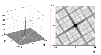
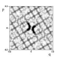
Figure 9: Husimi functions of quasimodes $|\Phi^{\rm cont}_{\phi=0}\rangle$ (left :3D linear scale; center: logarithmic scale) and $|\Phi^{\rm cont}_{\phi=2\lambda_{0}}\rangle$ (right, logarithmic scale) of the map $\hat{M}_{\rm Arnold}$ ($N=500$).

Sketch of proof.

We have to find an upper bound for the sum $\sum_{n\in\mathbb{Z}^{2},\>x+n\not\in B}|\Psi_{\phi,T}(x+n)|.$ We first consider the points $x+n$ in the sector $\mathcal{S}_{+}$; since they satisfy $|x+n|>>\sqrt{\hbar}$, the Bargmann function is described by formulas (• ‣ 6.1)–(80). As in Appendix 10.1, we split the region $\mathcal{S}_{+}\setminus B$ into a union of strips parallel to the unstable axis, of width $\delta p^{\prime}=\sqrt{\hbar}$. The results of Section 3.1 imply that two points $(x+n)$, $(x+m)$ in such a strip are separated by at least $|q^{\prime}(n-m)|\geq C_{o}\hbar^{-1/2}$. Summing the estimates (• ‣ 6.1,80) in these strips, we obtain the ($x$-independent) upper bound $\mathcal{O}(\sqrt{\hbar}T^{1/4})$ for points in $\mathcal{S}_{+}$. From (75), the sum over the three other sectors leads to the same bound. ∎

6.3 Controlling the speed of convergence

Using the pointwise formula (82), we can now directly compute the Fourier coefficients of the Husimi function of $|\Phi^{\rm cont}_{\phi}\rangle$:

$$\tilde{\mathcal{H}}_{\tilde{c}_{0},\Phi^{\rm cont}_{\phi}}(k)\stackrel{{\scriptstyle\rm def}}{{=}}\int_{\mathcal{F}}dx\,\rm e^{2{\rm i}\pi x\wedge k}\;N|\langle x,\tilde{c}_{0},\theta|\Phi^{\rm cont}_{\phi}\rangle|^{2},\quad k\in\mathbb{Z}^{2}.$$

We will prove the following estimate:

Proposition 9.

The Fourier coefficients of the (non-normalized) Husimi function for the quasimode $|\Phi^{\rm cont}_{\phi}\rangle$ satisfy, uniformly for $\phi$ in a bounded interval and $k\in\mathbb{Z}^{2}$, $|k|\leq\rm e^{\sqrt{T}}$:

$$\tilde{\mathcal{H}}_{\tilde{c}_{0},\Phi^{\rm cont}_{\phi}}(k)=S_{1}^{\rm cont}(\lambda,\phi)T\,(1+\delta_{k,0})+\mathcal{O}(\sqrt{T}).$$ (83)

This formula yields at the same time the norm of $|\Phi^{\rm cont}_{\phi}\rangle$, the convergence of the normalized quasimode to the measure $\frac{1+\delta_{0}}{2}$, but also the remainder $\mathcal{O}(T^{-1/2})$ in this convergence (which we could not obtain with previous methods). We do not know whether this estimate is sharp; in any case, we believe that the remainder cannot be smaller than $\mathcal{O}(T^{-1})$. Using the same methods, we can show that the remainder in the convergence of $|\Phi^{\rm cont}_{\rm loc}\rangle_{n}$ to its limit measure $\delta_{0}$ behaves as $F(k)T^{-1}$, with a function $F(k)\not\equiv 0$.

Proof.

From Eq. (82), we split $\mathcal{H}_{\tilde{c}_{0},\Phi_{\phi}}(x)$ into 3 components:

$$\mathcal{H}^{\rm diag}(x) =N\left(|\chi_{u}(x)\Psi_{\phi,T}(x+n_{u,x})|^{2}+|\chi_{s}(x)\Psi_{\phi,T}(x+n_{s,x})|^{2}\right)$$ (84)

$$\mathcal{H}^{\rm interf}(x) =N\left(\chi_{u}(x)\overline{\chi_{s}}(x)\Psi_{\phi,T}(x+n_{u,x})\overline{\Psi_{\phi,T}}(x+n_{s,x})\ +\ \ c.c.\ \ \right)$$ (85)

$$\mathcal{H}^{\rm remain}(x) =\mathcal{O}(\hbar^{-1/2}T^{1/4})\left(|\chi_{u}(x)\Psi_{\phi,T}(x+n_{u,x})|+|\chi_{s}(x)\Psi_{\phi,T}(x+n_{s,x})|\right)+\mathcal{O}(\sqrt{T}).$$ (86)

We will show that the integrals over $\mathcal{F}$ of the “remainder” and the “interference” components are $\mathcal{O}(T^{1/2})$, while the integral of $\rm e^{2{\rm i}\pi x\wedge k}\mathcal{H}^{\rm diag}(x)$ yields the dominant contribution in (83).

The integral of $\mathcal{H}^{\rm remain}$ on $\mathcal{F}$ is easy to treat. It involves $\int_{B}dx\,|\Psi_{\phi,T}(x)|$, which we estimate by using the asymptotics (• ‣ 6.1) in the domain $x\in B$, $|x|>>\sqrt{\hbar}$. This yields $\int_{B}dx|\Psi_{\phi,T}(x)|=\mathcal{O}(\hbar^{1/2}T^{-1/4})$, so the integral of $\mathcal{H}^{\rm remain}$ is an $\mathcal{O}(\sqrt{T})$.

Homoclinic intersections

To understand the “interference component” $\mathcal{H}^{\rm interf}(x)$, we have to describe a little bit the set $(B_{u}^{\mathbb{T}}\cap B_{s}^{\mathbb{T}})\setminus Sq$. It is composed of a large number of small “squares” surrounding homoclinic intersections (some of them are clearly visible in Fig. 9). Each of these squares is indexed by a couple of (nonzero and nonequal) integer vectors $(n_{u},n_{s})$ (finitely many such couples correspond to an actual square in $B^{\mathbb{T}}$):

$$Sq_{n_{u},n_{s}}\stackrel{{\scriptstyle\rm def}}{{=}}(B_{u}-n_{u})\cap(B_{s}-n_{s})=\{|q^{\prime}(x)+q^{\prime}(n_{s})|\leq 2\sqrt{\hbar T},\;|p^{\prime}(x)+p^{\prime}(n_{u})|\leq 2\sqrt{\hbar T}\}.$$

Since we have excluded the central square, one can use the asymptotics (• ‣ 6.1) for $\Psi_{\phi,T}(x+n_{u/s})$. The integral of $|\mathcal{H}^{\rm interf}(x)|$ on $Sq_{n_{u},n_{s}}$ is then smaller than

$$C\int_{Sq_{n_{u},n_{s}}}dq^{\prime}\,dp^{\prime}\,\frac{\hbar^{-1/2}}{\sqrt{|q^{\prime}(x+n_{u})p^{\prime}(x+n_{s})|}}\rm e^{-\frac{q^{\prime 2}(x+n_{s})}{2\hbar}}\rm e^{-\frac{p^{\prime 2}(x+n_{u})}{2\hbar}},$$

which admits the upper bound

$$\frac{C^{\prime}\hbar^{1/2}}{\sqrt{|q^{\prime}(n_{u}-n_{s})p^{\prime}(n_{s}-n_{u})|}}\leq C^{\prime}\hbar^{1/2}\left(\frac{1}{|q^{\prime}(n_{u}-n_{s})|}+\frac{1}{|p^{\prime}(n_{s}-n_{u})|}\right).$$

We now want to sum the RHS over all homoclinic squares in $B^{\mathbb{T}}$. To compute the sum over $1/q^{\prime}$ (resp. $1/p^{\prime}$), we consider the squares as subsets of $B_{u}$ (resp. $B_{s}$), which orders them along the strip. Two successive squares do not overlap, so their centers in $B_{u}$ (resp. in $B_{s}$) satisfy $|\delta q^{\prime}|\geq 4\sqrt{\hbar T}$. As a result, the total number of squares is less than $\frac{C}{\hbar T}$, and summing their contributions we get

$$\int_{\mathbb{T}}|\mathcal{H}^{\rm interf}(x)|\,dx\leq 4C^{\prime}\hbar^{1/2}\sum_{j=1}^{C/\hbar T}\frac{1}{j\,4\sqrt{\hbar T}}=\mathcal{O}\left(\frac{1}{\sqrt{T}}|\log(\hbar T)|\right)=\mathcal{O}(\sqrt{T}).$$

Notice that we ignored the phases present in $\mathcal{H}^{\rm interf}(x)$, as we had done in Section 4.3 to estimate $I(t,s)$.

Diagonal contribution

We now finish the proof by computing the integral

$$\int_{\mathcal{F}}dx\;\rm e^{2{\rm i}\pi x\wedge k}\mathcal{H}^{\rm diag}(x)=N\int_{B}dx\;\rm e^{2{\rm i}\pi x\wedge k}\;|\Psi_{\phi,T}(x)|^{2}.$$

The wedge product $2\pi x\wedge k$ is rewritten $k_{u}q^{\prime}+k_{s}p^{\prime}$ in the adapted coordinates. If $k\neq 0$, then $k_{u}=2\pi v_{+}\wedge k$, $k_{s}=2\pi v_{-}\wedge k$ are bounded away from zero (cf. Section 3.1).

We give some details for the computation of the integral in the positive sector $\mathcal{S}_{+}$. Let $\Theta(\hbar)$ be a semiclassically increasing function s.t. $1<<\Theta(\hbar)<<T^{1/4}$. The integral of $\mathcal{H}^{\rm diag}$ in the central region ($|q^{\prime}|<\Theta\sqrt{\hbar}$) admits the obvious upper bound $\mathcal{O}(\Theta^{2})$.

In the region $\{x\in\mathcal{S}_{+},\,q^{\prime}>\Theta\sqrt{\hbar}\}$, one can apply the asymptotics (79). After integrating over $p^{\prime}$, we obtain

$$\frac{S_{1}^{\rm cont}(\lambda,\phi)}{2\lambda}\int_{\Theta\sqrt{\hbar}}^{\frac{C_{o}}{9\sqrt{\hbar T}}}dq^{\prime}\;\frac{\rm e^{{\rm i}k_{u}q^{\prime}}}{q^{\prime}}\left(1+\mathcal{O}(\rm e^{-4T})+\mathcal{O}\Big{(}\frac{\hbar}{q^{\prime 2}}\Big{)}+\mathcal{O}(\hbar k_{s}^{2})\right).$$

This integral is easy to estimate:

• for $k=0$, it yields

  $$\frac{S_{1}^{\rm cont}(\lambda,\phi)}{2\lambda}\log\Big{(}\frac{C}{\hbar\sqrt{T}\Theta}\Big{)}+\mathcal{O}(\Theta^{-2})=\frac{S_{1}^{\rm cont}(\lambda,\phi)}{2}T+\mathcal{O}\big{(}\log(\Theta\sqrt{T})\big{)}.$$

• for $k\neq 0$, it has the asymptotics [BaHTF, Chap. 9]

  $$\frac{S_{1}^{\rm cont}(\lambda,\phi)}{2\lambda}|\log(\sqrt{\hbar}\Theta k_{u})|+\mathcal{O}(1)=\frac{S_{1}^{\rm cont}(\lambda,\phi)}{4}T+\mathcal{O}(\log(\Theta k_{u})).$$

Taking the 3 remaining sectors into account, we obtain the proposition. ∎

6.4 Husimi function close to the origin and $L^{s}$ norms

Besides providing the limit semiclassical measure, the pointwise formula (82) allows us to compute different indicators of localization for the quasimode $|\Phi_{\phi}^{\rm cont}\rangle_{n}$, namely the $L^{s}$ norms of its Husimi function [Pr, NV2]:

$$(s>0)\quad\|\mathcal{H}_{\Phi}\|_{s}\stackrel{{\scriptstyle\rm def}}{{=}}\left(\int_{\mathbb{T}}\left[\mathcal{H}_{\Phi}(x)\right]^{s}\,dx\right)^{1/s}.$$

For $s=2$, this defines a phase space analogy of the “inverse participation ratio” used in condensed-matter physics; in the limit $s\to 1^{+}$, it yields the Wehrl entropy of the state; for $s\to\infty$, this is sup-norm of the Husimi density.

Proposition 10.

For any fixed $\infty\geq s>1$ and $\phi$ in a bounded interval, the $L^{s}$ norms of the quasimodes $|\Phi^{\rm cont}_{\phi}\rangle_{n}$ behave in the semiclassical limit as

$$\left\|\mathcal{H}_{\tilde{c}_{0},|\Phi^{\rm cont}_{\phi}\rangle_{n}}\right\|_{s}\sim\frac{C(s,\phi/\lambda)}{\hbar^{1-\frac{1}{s}}|\log\hbar|}.$$

By comparison, the $L^{s}$-norms of a coherent state $|\tilde{c},\theta\rangle$ behave as $C^{\prime}(s,\tilde{c})\hbar^{-1+1/s}$ as $\hbar\to 0$, $\tilde{c}$ in a bounded set [NV2]. In the case of the sup-norm, we have a more precise statement (see Fig. 8):

Proposition 11.

For small enough $\hbar$, the maximum of $\mathcal{H}_{\tilde{c}_{0},|\Phi^{\rm cont}_{\phi}\rangle_{n}}(x)$ is at the origin for $|\phi|/\lambda<0.5$, and $C(\infty,\phi/\lambda)=\frac{|\Gamma(1/4+{\rm i}\phi/2\lambda)|^{2}}{2^{5/2}\pi^{3/2}}$. Conversely, for $|\phi|/\lambda>>1$, the maximum is close to the points $Q^{\prime}=-P^{\prime}=\pm\sqrt{\phi/\lambda}$ on the hyperbola, and $C(\infty,\phi/\lambda)\sim(2^{5/2}\sqrt{\pi|\phi|/\lambda})^{-1}$.

Sketch of proof.

For any $s>1$, the decrease $\sim\frac{1}{|x|^{s}}$ of the Husimi function along the hyperbola implies that most of the weight in the integral $\int_{\mathcal{F}}\mathcal{H}_{\Phi^{\rm cont}_{\phi}}^{s}$ is supported near the origin, so that this integral is close to $\int_{\mathbb{R}^{2}}\mathcal{H}_{\Psi^{(even)}_{\phi}}$. This yields the proposition, with the coefficients $C(s,\phi/\lambda)$ given as integrals of parabolic cylinder functions. The statements on the maxima derive from known results about parabolic cylinder functions. ∎

6.5 Odd-parity quasimodes

The connection (82) between torus quasimodes $|\Phi^{\rm cont}_{\phi}\rangle$ and generalized eigenstates $|\Psi^{(even)}_{\phi}\rangle$ hints at a property we have not used much, namely parity. We have already mentioned that for each energy $E=-\hbar\phi$, $\hat{H}$ admits two independent generalized eigenstates, $|\Psi^{(even)}_{\phi}\rangle$ of even parity, and a second one of odd parity, which we denote by $|\Psi^{(odd)}_{\phi}\rangle$. On the one hand, the Bargmann function of the latter can be expressed similarly as in Eq. (76):

$$\langle x,\tilde{c}_{0}|\Psi^{(odd)}_{\phi}\rangle=C^{\prime}_{\phi}\rm e^{-|Z|^{2}}\>\left\{D_{-1+2\mu}(2Z)-D_{-1+2\mu}(-2Z)\right\}.$$

On the other hand, as we did for $|\Psi^{(even)}_{\phi}\rangle$, we can build this odd eigenstate by propagating an “odd” coherent state at the origin, i.e. replacing the initial $|\tilde{c}_{0}\rangle$ in Eq. (72) by the first excited squeezed state

$$|\tilde{c}_{0}\rangle_{1}\stackrel{{\scriptstyle\rm def}}{{=}}\hat{M}_{(\tilde{c}_{0},0)}a^{\dagger}|0\rangle.$$

The Bargmann function of the corresponding quasimode $|\Psi_{\phi,T}\rangle_{1}$ is given by an integral similar to (73), with the integrand multiplied by the factor $\frac{Q^{\prime}-{\rm i}P^{\prime}}{\sqrt{2}\cosh\lambda s}$: this is therefore an odd function of $x$, semiclassically close to to $\langle x,\tilde{c}_{0}|\Psi^{(odd)}_{\phi}\rangle$

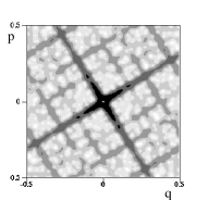
Figure 10: Husimi functions of the odd eigenstate $|\Psi^{(odd)}_{\phi=0}\rangle$ (linear scale) and the torus quasimode $|\Phi^{(odd)}_{\phi=0}\rangle$ (logarithmic scale) for $N=500$. Notice the zero at the origin.

Projecting this plane odd quasimode to the torus through $\hat{P}_{\theta}$, one obtains a quasimode $|\Phi^{(odd)}_{\phi}\rangle$ of $\hat{M}$ with quasiangle $\phi$. Provided one has selected periodicity conditions $\theta\equiv(0,0)\bmod\pi$, parity is conserved by $\hat{P}_{\theta}$, so that the Bargmann function $\langle x,\tilde{c}_{0},\theta|\Phi_{\phi}\rangle$ (resp. $\langle x,\tilde{c}_{0},\theta|\Phi^{(odd)}_{\phi}\rangle$) is an even (resp. an odd) function of $x$. As a result, these two quasimodes are mutually orthogonal. The Bargmann and Husimi functions of $|\Phi^{(odd)}_{\phi}\rangle$ can be described as precisely as for its even counterpart, in particular its normalized Husimi and Wigner functions converge as well to the measure $\frac{1+\delta_{0}}{2}$, with a remainder $\mathcal{O}(T^{-1/2})$.

6.6 On the “robustness” of continuous quasimodes

We want to show that the continuous quasimodes $|\Phi^{\rm cont}_{\phi}\rangle$, $|\Phi^{odd}_{\phi}\rangle$ are “stable” with respect to a change of the initial state ($|\tilde{c}_{0}\rangle$ and $|\tilde{c}_{0}\rangle_{1}$, respectively). One can indeed obtain an even quasimode very close to $|\Phi^{\rm cont}_{\phi}\rangle$ by propagating a different initial state $|\psi_{0}\rangle$: this state needs to be of even parity, sufficiently localized (e.g. a finite combination of excited coherent states), and taken away from a subspace of “bad” initial states. These remarks will be made more quantitative in Appendix 10.2, which treats the case where $|\psi_{0}\rangle$ is a squeezed coherent state of arbitrary squeezing.

To explain this “robustness”, we notice that the operator

$$\hat{\mathcal{P}}^{\rm cont}_{-\infty,\infty,\phi}\stackrel{{\scriptstyle\rm def}}{{=}}\int_{-\infty}^{\infty}ds\,\rm e^{-{\rm i}\phi s}\rm e^{-{\rm i}\hat{H}s/\hbar}$$

projects $L^{2}(\mathbb{R})$ onto the 2-dimensional space spanned by $|\Psi^{(even)}_{\phi}\rangle$ and $|\Psi^{(odd)}_{\phi}\rangle$. Any even state $|\psi_{0}\rangle\in L^{2}(\mathbb{R})$ will thus be projected onto $C_{\phi}(\psi_{0})|\Psi^{(even)}_{\phi}\rangle$, with the prefactor

$$C_{\phi}(\psi_{0})=\frac{\langle\Psi^{(even)}_{\phi}|\psi_{0}\rangle}{\langle\Psi^{(even)}_{\phi}|\tilde{c}_{0}\rangle}.$$

This prefactor vanishes iff there exists a state $|\varphi_{0}\rangle\in L^{2}(\mathbb{R})$ such that $|\psi_{0}\rangle=(\hat{H}+\nolinebreak\hbar\phi)|\varphi_{0}\rangle$; such $|\psi_{0}\rangle$ form a “bad” subspace of codimension $1$ inside the space of even states.

If $|\psi_{0}\rangle$ is localized inside a disk of radius $C\hbar^{1/2+\epsilon}$ at the origin, one can describe the plane quasimode $\hat{\mathcal{P}}^{\rm cont}_{-T,T,\phi}|\psi_{0}\rangle$ as in (77):

$$\langle x,\tilde{c}_{0}|\hat{\mathcal{P}}^{\rm cont}_{-T,T,\phi}|\psi_{0}\rangle=C_{\phi}(\psi_{0})\langle x,\tilde{c}_{0}|\Psi^{(even)}_{\phi}\rangle+\mathcal{O}(\hbar^{1/2-\epsilon})\quad\mbox{uniformly in $x\in\mathbb{R}^{2}$}.$$ (87)

If $C_{\phi}(\psi_{0})$ is of order unity, this estimate shows that $\hat{\mathcal{P}}^{\rm cont}_{-T,T,\phi}|\psi_{0}\rangle$ resembles the quasimode $|\Psi_{\phi,T}\rangle$. One can then show (as in Section 6.2) that the torus state $\hat{P}_{\theta}\hat{\mathcal{P}}^{\rm cont}_{-T,T,\phi}|\psi_{0}\rangle$ is close to the quasimode $C_{\phi}(\psi_{0})|\Phi^{\rm cont}_{\phi}\rangle$.

As an example, consider the case $\phi=0$: one can start from any (finitely) excited coherent state of the form $|\tilde{c}_{0}\rangle_{4n}\propto\hat{M}_{(\tilde{c}_{0},0)}\big{(}a^{\dagger}\big{)}^{4n}|0\rangle$ to obtain a quasimode asymptotically close to $|\Phi^{\rm cont}_{0}\rangle$. On the opposite, the states $|\tilde{c}_{0}\rangle_{4n+2}$ are “bad” initial states, because they are in the range of $\hat{H}$.

This discussion straightforwardly transposes to the construction of the odd quasimodes $|\Phi^{odd}_{\phi}\rangle$ starting from odd localized states.

7 Quasimodes on a general periodic orbit

We have so far described the construction of quasimodes localized on the fixed point $0$ of the classical map $M$. We will now generalize this construction to a general periodic orbit of $M$. The associated Husimi densities will be shown to be (semiclassically) partly localized on the orbit and partly equidistributed. The proofs require some minor changes with respect to the previous case, but no fundamentally new ingredients.

We consider a fixed periodic orbit $\mathcal{P}=\left\{x_{\ell}\in{\mathcal{F}}\right\}^{\tau}_{\ell=0}$ of (primitive) period $\tau$, in other words, for $0\leq\ell<\tau$, $Mx_{\ell}=x_{\ell+1}$ mod $\mathbb{Z}^{2}$ and $x_{\tau}=x_{0}$. Note that $M^{\tau}x_{\ell}=x_{\ell}\ \mathrm{mod}\ \mathbb{Z}^{2}$, so that all $x_{\ell}$, when viewed as points on the torus, are fixed points of $M^{\prime}\stackrel{{\scriptstyle\rm def}}{{=}}M^{\tau}$. Furthermore, for all $0\leq\ell\leq\tau$, there exist $m_{\ell}\in\mathbb{Z}^{2}$ so that

$$x_{\ell}=M^{\ell}x_{0}-m_{\ell}.$$

We will first introduce the discrete time quasimode defined in (2) and will consider its continuous time analog below:

$$|\Phi^{\rm disc}_{\phi}\rangle=\sum_{t=-T}^{T-1}\rm e^{-{\rm i}\phi t}\hat{M}^{t}\hat{P}_{\theta}\hat{T}_{x_{0}}|\tilde{c}_{0}\rangle.$$

Letting $T$ be the integer multiple of $\tau$ that is closest to $|\ln\hbar|/\lambda$, and setting $T^{\prime}=T/\tau$, a simple computation yields

$$|\Phi_{\phi}^{\rm disc}\rangle=\sum_{\ell=0}^{\tau-1}\rm e^{-{\rm i}\phi\ell}|\Phi^{\rm disc}_{\ell}\rangle\quad\mathrm{where}\quad|\Phi_{\ell}^{\rm disc}\rangle=\hat{M}^{\ell}\left(\sum_{k=-T^{\prime}}^{T^{\prime}-1}\rm e^{-{\rm i}\phi\tau k}\hat{M^{\prime}}^{k}\right)\hat{P}_{\theta}\hat{T}_{x_{0}}|\tilde{c}_{0}\rangle.$$ (88)

It is easy to see that

$$\hat{M}^{\ell}\hat{P}_{\theta}\hat{T}_{x_{0}}=\hat{P}_{\theta}\hat{T}_{x_{\ell}+m_{\ell}}\hat{M}^{\ell}=\rm e^{{\rm i}S_{\ell}}\hat{P}_{\theta}\hat{T}_{x_{\ell}}\hat{M}^{\ell},$$ (89)

where $S_{\ell}=\theta\cdot m_{l}+{\rm i}\delta_{m_{l}}+{\rm i}\pi Nm_{l}\wedge x_{l}$ (see (19)). This phase can partly be interpreted in terms of the action along the classical orbit; however, the $\theta$-term is non-classical, akin to the quantum phase due to a pointwise magnetic flux tube on a charged particle (Aharonov-Bohm effect) [KM]. Hence

$$|\Phi_{\ell}^{\rm disc}\rangle=\rm e^{{\rm i}S_{\ell}}\left(\sum_{k=-T^{\prime}}^{T^{\prime}-1}\rm e^{-{\rm i}\phi\tau k}\hat{M^{\prime}}^{k}\right)\hat{P}_{\theta}\hat{T}_{x_{\ell}}\hat{M}^{\ell}|\tilde{c}_{0}\rangle.$$ (90)

This suggests that $|\Phi_{\ell}^{\rm disc}\rangle$ is a quasimode of quasiangle $\phi\tau$ for $\hat{M}^{\prime}$, associated to the fixed point $x_{\ell}$ of $M^{\prime}$. This is basically the content of Proposition 12. There is another instructive way of rewriting $|\Phi_{\ell}^{\rm disc}\rangle$ which corroborates this idea. For that purpose, we first draw from Eq. (89)

$$\hat{M}^{\tau k}\hat{P}_{\theta}\hat{T}_{x_{0}}=\rm e^{{\rm i}kS_{\tau}}\hat{P}_{\theta}\hat{T}_{x_{0}}\hat{M}^{\tau k}\quad\mathrm{and}\quad\hat{M}^{\tau k+\ell}\hat{P}_{\theta}\hat{T}_{x_{0}}=\rm e^{{\rm i}(kS_{\tau}+S_{\ell})}\hat{P}_{\theta}\hat{T}_{x_{\ell}}\hat{M}^{\tau k+\ell}.$$ (91)

Using this, one can write

$$|\Phi_{\ell}^{\rm disc}\rangle=\rm e^{{\rm i}S_{\ell}}\hat{T}_{x_{\ell}}\hat{P}_{\tilde{\theta}_{\ell}}\left(\sum_{k=-T^{\prime}}^{T^{\prime}-1}\rm e^{-{\rm i}(\phi\tau-S_{\tau})k}\hat{M^{\prime}}^{k}\right)\hat{M}^{\ell}|\tilde{c}_{0}\rangle,$$ (92)

where we used $\hat{P}_{\theta}\hat{T}_{x_{\ell}}=\hat{T}_{x_{\ell}}\hat{P}_{\tilde{\theta}_{\ell}}$ with $\tilde{\theta}_{\ell}=\theta+2\pi N(p_{\ell},-q_{\ell})$. A simple computation shows that, because $x_{\ell}$ is a fixed point for $M^{\tau}$, $\tilde{\theta}_{\ell}$ is a fixed point for the map $\theta\to\theta^{\prime}$ defined in (31), with $M$ replaced by $M^{\prime}$. Consequently, $|\Phi^{\rm disc}_{\phi}\rangle$ is the $x_{\ell}$ translate of a quasimode for $\hat{M}^{\prime}$ at the origin with quasiangle $\phi\tau-S_{\tau}$, of the type studied in the previous sections.

To build continuous time quasimodes, we replace in all the above formulas $|\tilde{c}_{0}\rangle$ by

$$\frac{1}{\tau}\int_{0}^{\tau}dt\,\rm e^{-{\rm i}t\tilde{\phi}}\,\rm e^{-\frac{{\rm i}}{\hbar}\hat{H}t}|\tilde{c}_{0}\rangle,$$ (93)

where the “quasienergy” $\tilde{\phi}\in\mathbb{R}$ is chosen so that

$$\tau\tilde{\phi}\equiv\tau\phi-S_{\tau}\bmod{2\pi}.$$ (94)

Whereas the quasiangle $\phi$ is defined modulo $2\pi$, the quasienergy $\tilde{\phi}$ is chosen in $\mathbb{R}$. The continuous quasimode reads:

$$|\Phi_{\ell}^{\rm cont}\rangle=\rm e^{{\rm i}S_{\ell}}\hat{T}_{x_{\ell}}\hat{P}_{\tilde{\theta}_{\ell}}\ \frac{1}{\tau}\int_{-T}^{T}dt\,\rm e^{-{\rm i}\tilde{\phi}t}\rm e^{-\frac{{\rm i}}{\hbar}\hat{H}t}\hat{M}^{\ell}|\tilde{c}_{0}\rangle.$$ (95)

All the above quasimodes can of course in obvious ways be split into a localized and an equidistributing part, as before. For both the discrete and continuous time quasimodes we have the following estimates:

Proposition 12.

For all $0\leq\ell^{\prime}<\ell\leq\tau-1$, for all $f\in C_{0}^{\infty}(\mathbb{T}^{2})$, for all $k\in\mathbb{Z}$,

$$\langle\Phi_{\ell}|\Phi_{\ell}\rangle = 2T^{\prime}S_{1}(\phi\tau-S_{\tau},\tau\lambda)+\mathcal{O}(1)$$ (96)

$$\lim_{\hbar\to 0}\ {}_{n}\!\langle\Phi_{\ell}|\hat{f}|\Phi_{\ell}\rangle_{n} = \frac{1}{2}f(x_{\ell})+\frac{1}{2}\int_{\mathbb{T}^{2}}f(x)dx.$$ (97)

$$\lim_{\hbar\to 0}\ {}_{n}\!\langle\Phi_{\ell^{\prime}}|\hat{T}_{k/N}|\Phi_{\ell}\rangle_{n} = 0$$ (98)

The quasimodes $|\Phi_{\phi}\rangle$ satisfy (7), the limit being uniform for $\phi$, $\tilde{\phi}$ in a bounded interval.

Starting from (95) a pointwise analysis of the continuous time quasimode $|\Phi^{\rm cont}_{\mathcal{P},\phi}\rangle$ can be performed as well, along the lines of Section 6.2. One should notice that the Husimi function of $|\Phi^{\rm cont}_{\mathcal{P},\phi}\rangle$ in the $\sqrt{\hbar}$-vicinity of a periodic point $x_{l}$ is dominated by the contribution of $|\Phi_{l}^{\rm cont}\rangle$; it is concentrated on a hyperbola which depends on the quasienergy $\tilde{\phi}$ rather than on the quasiangle $\phi$.

Proof of the proposition.

We write the proof for the discrete time quasimodes only. (92) immediately implies (96) and (97) as a consequence of the results of Section 5. To prove (98) when $k=0$, i.e. the asymptotic orthogonality of the $|\Phi_{\ell}\rangle$, we write, using (88) and (91)

$$\!\langle\Phi_{\ell^{\prime}}^{\rm disc}|\Phi_{\ell}^{\rm disc}\rangle=\sum_{k^{\prime}=-T^{\prime}}^{T^{\prime}-1}\sum_{k=-T^{\prime}}^{T^{\prime}-1}\rm e^{-{\rm i}(\phi\tau-S_{\tau})(k-k^{\prime})+{\rm i}S_{\ell-\ell^{\prime}}}\langle\tilde{c}_{0}|\hat{T}_{-x_{0}}\hat{P}_{\theta}\hat{T}_{x_{\ell-\ell^{\prime}}}\hat{M}^{(\ell-\ell^{\prime})+\tau(k-k^{\prime})}|\tilde{c}_{0}\rangle,$$

so that

$$\begin{split}\big{|}\langle\Phi_{\ell^{\prime}}^{\rm disc}|\Phi_{\ell}^{\rm disc}\rangle\big{|}&\leq\sum_{k^{\prime}=-T^{\prime}}^{T^{\prime}-1}\sum_{k=-T^{\prime}}^{T^{\prime}-1}\sum_{m\in\mathbb{Z}^{2}}|\langle\tilde{c}_{0}|\hat{T}_{-x_{0}}\hat{T}_{m}\hat{T}_{x_{\ell-\ell^{\prime}}}\hat{M}^{(\ell-\ell^{\prime})+\tau(k-k^{\prime})}|\tilde{c}_{0}\rangle|\\ &\leq\sum_{k^{\prime}=-T^{\prime}}^{T^{\prime}-1}\sum_{k=-T^{\prime}}^{T^{\prime}-1}J_{r}(\tau(k-k^{\prime})+\ell-\ell^{\prime},0)\leq C,\end{split}$$ (99)

where $r=x_{0}-x_{\ell-\ell^{\prime}}$, and where we used the estimate $J_{r}(t,0)\leq C\hbar\rm e^{\lambda|t|/2}$ extracted from Appendix 10.1. To prove (98) when $k\not=0$, one repeats the arguments of Section 5: we omit the details. For continuous quasimodes, the proofs are analogous, using this time the same estimate on $J_{r}(t,s)$. The proof of (7) follows immediately. ∎

Convex combinations of limit measures

We can further enlarge the set of semiclassical limit measures by taking finite convex combinations of the previous ones. Consider a finite set of periodic orbits $\{\mathcal{P}_{1},\ldots,\mathcal{P}_{f}\}$, and complex coefficients $\{\alpha_{1},\ldots,\alpha_{f}\}$ satisfying $\sum_{i=1}^{f}|\alpha_{i}|^{2}=1$. Let $|\Phi_{\mathcal{P}_{i},\phi}\rangle$ be quasimodes (discrete or continuous time ) associated to $\mathcal{P}_{i}$, as defined above, with the same quasiangle $\phi$. We can then combine them into the quasimode

$$|\Phi\rangle\stackrel{{\scriptstyle\rm def}}{{=}}\sum_{i=1}^{f}\alpha_{i}\,|\Phi_{\mathcal{P}_{i},\phi}\rangle_{n}.$$

One readily shows along the lines of the proof of Proposition 12 that for $i\not=j$, and for all $k\in\mathbb{Z}^{2}$, one has

$$\lim_{\hbar\to 0}\ {}_{n}\langle\Phi_{\mathcal{P}_{i}}|\hat{T}_{k/N}|\Phi_{\mathcal{P}_{j}}\rangle_{n}=0.$$

This together with (7) shows that the Husimi and Wigner functions of $|\Phi\rangle_{n}$ converge to the limit measure $\frac{1}{2}\left(dx+\sum_{i=1}^{f}|\alpha_{i}|^{2}\,\delta_{\mathcal{P}_{i}}\right)$.

8 Scarred eigenstates for quantum cat maps of short quantum periods

We will now slightly extend an argument from [BonDB1] in order to show that the quasimodes we have built and studied in the previous sections are exact eigenstates of the quantum map $\hat{M}$ for certain special values of $\hbar$ and we will prove Theorem 1.

For that purpose, we first recall a few facts about quantum cat maps [HB]. For a given value of $N=(2\pi\hbar)^{-1}$, every quantum map $\hat{M}$ has a “quantum period” $P(N)$ defined to be the smallest nonnegative integer such that

$$\hat{M}^{P(N)}=\rm e^{i\varphi(N)}\hat{I}_{{\cal H}_{N,\theta}}\quad\textrm{for a certain }\varphi(N)\in[-\pi,\pi[.$$ (100)

It follows that, if $\phi$ is of the type $\phi=\phi_{j}=\frac{\varphi(N)+2\pi j}{P(N)}$, then $\frac{1}{P(N)}\hat{\mathcal{P}}_{t_{1},t_{1}+P(N),\phi_{j}}$ is independent of $t_{1}$, and is the spectral projector onto the eigenspace of $\hat{M}$ inside ${\cal H}_{N,\theta}$ associated to the eigenvalue $\rm e^{{\rm i}\phi_{j}}$ (the normalization factor $1/P(N)$ ensures that it is indeed a projector). All eigenvalues of $\hat{M}$ on ${\cal H}_{N,\theta}$ are necessarily of that form.

The function $P(N)$ depends on $N$ in an erratic way, and no closed formula exists for it [Ke]. It satisfies the general bounds

$$\exists C>0,\quad\forall N\in\mathbb{N}^{*},\quad\frac{2}{\lambda}\log N-C\leq P(N)\leq C\;N\log\log N.$$ (101)

It is moreover known that, for “almost all” integers, $P(N)\geq\sqrt{N}$ [KR2]. We will now give an elementary argument to show that, given any hyperbolic matrix in SL$(2,\mathbb{Z})$, there exists an infinite sequence of integers $N_{k}$ for which the quantum period is very short in the sense that it saturates the above lower bound:

$$P(N_{k})=2\frac{\log N_{k}}{\lambda}+\mathcal{O}(1)=2T_{k}+\mathcal{O}(1),$$ (102)

where the Ehrenfest time $T$ was defined in (45).

Let us first recall that, for all $k\in\mathbb{N}^{*}$, one has

$$M^{k}=p_{k}M-p_{k-1},\quad\mathrm{where}\quad p_{k}=\frac{\rm e^{\lambda k}-\rm e^{-\lambda k}}{\rm e^{\lambda}-\rm e^{-\lambda}},\ p_{0}=0.$$

It was proven in [BonDB1] that, for all $k\geq 1$, the integer $\tilde{N}_{k}=\mathrm{GCD}(p_{k},p_{k-1}+1)$ satisfies

$$\frac{2}{\lambda}\log\tilde{N}_{k}=k+\mathcal{O}(1),$$ (103)

and that

$$M^{k}=I+\tilde{N}_{k}M_{k},\quad\mbox{with $M_{k}$ an integer matrix}.$$ (104)

We now set $N_{k}=\tilde{N}_{k}$ if $\tilde{N}_{k}$ is odd, $N_{k}=\tilde{N}_{k}/2$ if $\tilde{N}_{k}$ is even. Choosing the periodicity angle $\theta=(0,0)$ when $N_{k}$ is even and $\theta=(\pi,\pi)$ when $N_{k}$ is odd (which makes sense, cf. the end of Section 3.2), we prove below the following lemma:

Lemma 4.

With $N_{k}$, $\theta$ given as above, $\hat{M}^{k}=\rm e^{i\varphi}\hat{I}_{\mathcal{H}_{N_{k},\theta}}\quad$ for a certain $\varphi\in[-\pi,\pi[$.

This means that the quantum period $P(N_{k})$ of $\hat{M}$ on $\mathcal{H}_{N_{k},\theta}$ divides $k$. Comparing (101) with (103) entails that for $k$ large enough, $P(N_{k})=k$ and (102) holds.

Proof of the lemma.

The case $\tilde{N}_{k}=2N_{k}$, $\theta=(0,0)$ was treated in [HB]. We give a different proof, which works for both cases.

From Schur’s Lemma and the irreducibility of the $\hat{T}_{n/N_{k}}$, it suffices to show that $\left[\hat{M}^{k},\hat{T}_{n/N_{k}}\right]=0$ on $\mathcal{H}_{N_{k},\theta}$, for all $n\in\mathbb{Z}^{2}$. Setting $\tilde{N}_{k}=\epsilon N_{k}$, $\theta=\epsilon^{\prime}(\pi,\pi)$ and using the definition of $\hat{P}_{\theta}$, Eqs. (19) and (20), one readily computes

$$\hat{M}^{k}\hat{T}_{n/N_{k}}\hat{M}^{-k}\hat{P}_{\theta} =\rm e^{i\pi\epsilon(n\wedge M_{k}n)}\hat{T}_{n/N_{k}}\hat{T}_{M_{k}n}\hat{P}_{\theta}$$

$$=(-1)^{\epsilon(n\wedge M_{k}n)+\epsilon\epsilon^{\prime}[(M_{k}n)_{1}+(M_{k}n)_{2}+(M_{k}n)_{1}(M_{k}n)_{2}]}\hat{T}_{n/N_{k}}\hat{P}_{\theta}.$$

This phase is trivial if $\epsilon=2$. In the case $\epsilon=\epsilon^{\prime}=1$ (that is, $\tilde{N}_{k}$ odd), one must consider the $6$ possible values of $M$ modulo $2$: in all cases, the phase is trivial. ∎

If we now consider such a value $N_{k}$ together with an admissible eigenangle $\phi_{j_{k}}$, the eigenstates

$$|\Phi_{k}\rangle=\sum_{t=-P(N_{k})/2}^{P(N_{k})/2-1}\rm e^{-{\rm i}\phi_{j_{k}}t}\hat{M}^{t}|x_{0},\tilde{c}_{0}\rangle$$

are (discrete time) quasimodes of the quantum map as studied in the previous sections. Indeed, as discussed at the end of Section 5, since $T$ and $P(N_{k})/2$ differ by a bounded number of terms in the semiclassical limit, we can replace one by the other in (2), without affecting any of the semiclassical properties of the quasimodes. One can similarly construct eigenfunctions that are continuous time quasimodes.

Proof of Theorem 1.

The previous arguments settle the case $\beta=1/2$. To treat the general case, we recall that the Schnirelman theorem implies the existence of a sequence of eigenfunctions $|\varphi_{k}\rangle_{n}$ of $\hat{M}$ on $\mathcal{H}_{N_{k},\theta}$ (with corresponding eigenvalues $(\phi_{j_{k}})_{k\in\mathbb{N}}$) that equidistribute as $k\to\infty$. We then construct, for $0\leq\alpha\leq 1$:

$$|\psi_{k}\rangle=\alpha|\Phi_{k}\rangle_{n}+\sqrt{1-\alpha^{2}}|\varphi_{k}\rangle_{n}$$

If we show that, for all $n\in\mathbb{Z}^{2}$,

$$\lim_{\hbar\to 0}\ {}_{n}\!\langle\varphi_{k}|\hat{T}_{n/N_{k}}|\Phi_{k}\rangle_{n}=0,$$

a simple computation implies that the $|\psi_{k}\rangle_{n}$ satisfy (8) with $\beta=\alpha^{2}/2$. We have

$$\lim_{\hbar\to 0}\ {}_{n}\!\langle\varphi_{k}|\hat{T}_{n/N_{k}}|\Phi_{k}\rangle_{n}=\lim_{\hbar\to 0}\left(\ {}_{n}\!\langle\varphi_{k}|\hat{T}_{n/N_{k}}|\Phi_{k,\mathrm{erg}}\rangle_{n}+\ _{n}\!\langle\varphi_{k}|\hat{T}_{n/N_{k}}|\Phi_{k,\mathrm{loc}}\rangle_{n}\right).$$

The second limit vanishes with an argument as in (71), whereas for the first, we use the further decomposition $|\Phi_{k,\mathrm{erg}}\rangle=|\Phi_{k,1}\rangle+|\Phi_{k,4}\rangle$ with $|\Phi_{k,1}\rangle=\rm e^{{\rm i}\phi_{j_{k}}T/2}\hat{M}^{-T/2}|\Phi_{k,2}\rangle$, $|\Phi_{k,4}\rangle=\rm e^{-{\rm i}\phi_{j_{k}}T/2}\hat{M}^{T/2}|\Phi_{k,3}\rangle$ (see (3)). Now, since $|\varphi_{j_{k}}\rangle_{n}$ is an eigenfunction, we have

$$\big{|}\,_{n}\!\langle\varphi_{k}|\hat{T}_{n/N_{k}}|\Phi_{k,4}\rangle_{n}\big{|}=\big{|}\,_{n}\!\langle\varphi_{k}|\hat{M}^{-T/2}\hat{T}_{n/N_{k}}\hat{M}^{T/2}|\Phi_{k,3}\rangle_{n}\big{|}.$$

As in the proof of Proposition 6, and more specifically Eq. (71), this tends to $0$ with $\hbar$. ∎

For matrices $M$ of “checkerboard structure”, the results of [KR1, Me] imply that, given an arbitrary sequence of eigenvalues $(\phi_{j_{k}})_{k\in\mathbb{N}}$, there exists a corresponding sequence of eigenvectors $|\varphi_{k}\rangle\in\mathcal{H}_{N_{k},\theta}$ that semiclassically equidistribute. One can then construct for the same eigenvalues eigenstates $|\psi_{k}\rangle$ satisfying Eq. (8).

The $P(N_{k})$ eigenstates with distinct eigenvalues constructed above are of course exactly orthogonal to each other, and not just asymptotically as proven in Section 5.3. On the other hand, two continuous time eigenstates of identical eigenangle $\phi_{j}$ but different quasienergies $\tilde{\phi}-\tilde{\phi}^{\prime}=s\pi/T$, $s\neq 0$ become orthogonal in the semiclassical limit. This is also the case for two eigenstates with the same eigenangle supported on different periodic orbits $\mathcal{P}\neq\mathcal{P}^{\prime}$.

9 Conclusion

In this article we have constructed and analyzed a certain class of “quasimodes” of hyperbolic quantized torus isomorphisms, which for certain values of $\hbar$ become exact eigenstates. The characteristic property of these quasimodes is that their “quantum limit”, that is the weak limit of their Husimi densities, does not yield the Liouville measure, but contains a singular component supported on a (finite union of) periodic orbit(s). In our case, this singular component has a relative weight $\beta\leq 1/2$, less than or equal to the weight of the Liouville part. As explained in the introduction, no limit measure of eigenstates can have a “larger” singular component. We further conjecture that no sequence of quasimodes (i.e. images of the operators $\mathcal{\hat{P}}_{-T,T,\phi}$) can have a more singular limit measure either.

The strong scarring of eigenstates exhibited in this paper is directly linked to the very large degeneracies of the eigenvalues of $\hat{M}$ for certain special values of Planck’s constant. Therefore, such sequences of eigenstates are very probably absent as soon as one considers nonlinear perturbations of the dynamics, for instance $\hat{M}_{\epsilon}=\rm e^{-{\rm i}\epsilon\hat{H}_{1}/\hbar}\hat{M}$, for any periodic Hamiltonian $H_{1}(x)$ and $\epsilon>0$ small enough. Such a perturbation of the classical map is known to conserve the uniform hyperbolicity, but destroys the “action degeneracies” characteristic of the (linear) cat map. As a consequence the spectrum of the perturbed map exhibits Random Matrix statistics, in particular “repulsion” between eigenangles [KM], which forbids degeneracies.

The precise characterization of some weaker form of scarring for individual eigenstates that would remain valid for $\hat{M}_{\epsilon}$ remains therefore an open problem. Nevertheless, it might be interesting to study the phase space distribution of the “nonlinear“ quasimodes of the type $\sum_{t=-T}^{T}\rm e^{-{\rm i}\phi t}\hat{M}^{t}_{\epsilon}|x_{0},\tilde{c}\rangle$, for $x_{0}$ a periodic point of $M_{\epsilon}$, which may not be as simple to describe as for the linear map.

Acknowledgments:

We have benefited from useful conversations with Y. Colin de Verdière, C. Gérard, E. Vergini, A. Voros, D. Wisniacki. F. F. acknowledges the kind hospitality of the Service de Physique Théorique, CEA Saclay where part of this work was accomplished.

10 Appendices

10.1 Estimate of the interference term $I(t,s)$

In this appendix we prove Proposition 1. For the purpose of Section 7 we will at the same time give a bound for the more general overlap ($t,s\in\mathbb{R}$)

$$\left|\langle r,\tilde{c}_{s}|\hat{P}_{\theta}\,\rm e^{-{\rm i}\hat{H}t/\hbar}|\tilde{c}_{s}\rangle\right|\leq\sum_{n\in\mathbb{Z}^{2}}\left|\langle r+n,\tilde{c}_{s}|\rm e^{-\frac{i}{\hbar}\hat{H}t}|\tilde{c}_{s}\rangle\right|,$$ (105)

where $r\in\mathcal{F}$ (the fundamental domain) belongs to the lattice $\left(\frac{1}{D}\mathbb{Z}\right)^{2}$, with $D\in\mathbb{N}^{*}$ and where $\theta\in[0,2\pi[\times[0,2\pi[$ is arbitrary (in other words, $\theta$ need not be equal to the fixed point of the map (31). We define

$$J_{r}(t,s)\stackrel{{\scriptstyle\rm def}}{{=}}\sum_{n\in\mathbb{Z}^{2},r+n\not=0}\left|\langle r+n,\tilde{c}_{s}|\rm e^{-\frac{i}{\hbar}\hat{H}t}|\tilde{c}_{s}\rangle\right|.$$ (106)

We first consider the case $s=0$, $t\geq 0$. Since $\sqrt{\hbar}\leq\Delta p^{\prime}\leq\sqrt{2\hbar}$ for all positive times, only the points $r+n$ near the unstable axis can significantly contribute. Therefore, we subdivide the plane into strips parallel to this axis: the “outer” strips

$$\forall l\geq 1,\quad S_{\pm l}=\left\{x\mid a_{l}\leq\pm p^{\prime}(x)<a_{l+1}\right\},$$

with $a_{l}=W_{0}+(l-1)W$, and the central strip $S_{0}=\left\{x\neq 0\mid p^{\prime}(x)|<W_{0}\right\}$. The widths $W_{0},\>W$ will be explicitly set below.

We start by estimating the contribution of the points $r+n\in S_{l}$ with $l\geq 1$. Due to the diophantine condition (25), as long as $W$ is small enough, two points in this strip satisfy the property $|q^{\prime}(r+n)-q^{\prime}(r+m)|>C_{o}/W$. Ordering these points according to their abscissas: $q^{\prime}(r+n_{j})<q^{\prime}(r+n_{j+1})<q^{\prime}(r+n_{j+2})$, we have for any $\alpha>0$ :

$$\sum_{j\in\mathbb{Z}}\exp\left\{-\alpha q^{\prime}(r+n_{j})^{2}\right\}\leq\sum_{j\in\mathbb{Z}}\exp\left\{-\alpha\left(\frac{jC_{o}}{W}\right)^{2}\right\}.$$ (107)

The sum on the RHS is a one-dimensional theta function, which has the upper bound (optimal for $0<\alpha$ small enough):

$$\sum_{j\in\mathbb{Z}}\rm e^{-\alpha j^{2}}\leq 1+\sqrt{\frac{\pi}{\alpha}}.$$ (108)

As a result, using (43) it becomes clear that the contribution to $J_{r}(t)$ of the points $r+n\in S_{l}$ is bounded above by

$$\sum_{r+n_{j}\in S_{l}}\frac{1}{\sqrt{\cosh\lambda t}}\;\exp\left\{-\frac{1}{2}\left[\frac{p^{\prime}(r+n_{j})^{2}}{\Delta p^{\prime 2}}+\frac{q^{\prime}(r+n_{j})^{2}}{\Delta q^{\prime 2}}\right]\right\}\\ \leq\sqrt{2}\rm e^{-\lambda t/2}\,\rm e^{-\frac{a_{l}^{2}}{2\Delta p^{\prime 2}}}\,\left[1+\sqrt{2\pi}\frac{W\Delta q^{\prime}}{C_{o}}\right].$$ (109)

The estimate (108) can then be applied to the sum over the strips $S_{l}$, $l\neq 0$, to obtain (remind $|t;\tilde{c}_{0}\rangle=\rm e^{-{\rm i}\hat{H}t/\hbar}|\tilde{c}_{0}\rangle$)

$$\sum_{l\neq 0}\>\sum_{r+n\in S_{l}}\left|\langle r+n,\tilde{c}_{0}|t;\tilde{c}_{0}\rangle\right|\leq\sqrt{2}\rm e^{-\lambda t/2}\,\rm e^{-\frac{W_{0}^{2}}{2\Delta p^{\prime 2}}}\,\left[2+\frac{\sqrt{2\pi}\Delta p^{\prime}}{W}\right]\,\left[1+\frac{\sqrt{2\pi}W\Delta q^{\prime}}{C_{o}}\right].$$

For each time $t$, we can minimize the RHS with respect to $W$ by taking $W^{2}=C_{o}\frac{\Delta p^{\prime}}{2\Delta q^{\prime}}=\frac{C_{o}}{2}\rm e^{-\lambda t}$, which leads to the bound

$$\sum_{l\neq 0}\>\sum_{r+n\in S_{l}}\left|\langle r+n,\tilde{c}_{0}|t;\tilde{c}_{0}\rangle\right|\leq 2\sqrt{2}\rm e^{-\frac{W_{0}^{2}}{2\Delta p^{\prime 2}}}\,\rm e^{-\lambda t/2}\,\left[1+\sqrt{\frac{\pi}{C_{o}}}\Delta p^{\prime}\rm e^{\lambda t/2}\right]^{2}.$$ (110)

Notice that this upper bound is independent of the point $r$.

We now estimate the contribution of the strip $S_{0}$, which requires more care, and will depend on $r$. For any point $r^{\prime}\neq 0$ on the lattice $\left(\frac{1}{D}\mathbb{Z}\right)^{2}$ sufficiently close to the unstable axis, the diophantine property (25) implies $|p^{\prime}(r^{\prime})|\geq\frac{C_{o}}{D^{2}|q^{\prime}(r^{\prime})|}$. As a consequence, the quadratic form appearing in (43) may be bounded inside $S_{0}$ by

$$\frac{q^{\prime}(r+n)^{2}}{2\Delta q^{\prime 2}}+\frac{p^{\prime}(r+n)^{2}}{2\Delta p^{\prime 2}}\geq\frac{q^{\prime}(r+n)^{2}}{2\Delta q^{\prime 2}}+\frac{C_{o}^{2}}{2D^{4}\Delta p^{\prime 2}\,q^{\prime}(r+n)^{2}}\stackrel{{\scriptstyle\rm def}}{{=}}f_{t}(q^{\prime}(r+n)).$$ (111)

The function $f_{t}$ satisfies the scaling property $f_{t}(q)=\frac{C_{o}\rm e^{-\lambda t}}{2D^{2}\Delta p^{\prime 2}}\,f\left(\frac{qD\rm e^{-\lambda t/2}}{\sqrt{C_{o}}}\right)$, with $f(q)\stackrel{{\scriptstyle\rm def}}{{=}}q^{2}+q^{-2}$. This function $f(q)$ is bounded below for all positive $q$ by the parabola $g(q)=2+(q-1)^{2}$, so after rescaling we get

$$\forall q>0,\quad f_{t}(q)\geq g_{t}(q)\stackrel{{\scriptstyle\rm def}}{{=}}\frac{C_{o}\rm e^{-\lambda t}}{D^{2}\Delta p^{\prime 2}}+\frac{\rm e^{-2\lambda t}}{2\Delta p^{\prime 2}}\left(q-\sqrt{C_{o}}\rm e^{\lambda t/2}/D\right)^{2}.$$

We consider the contributions of the points $r+n$ in $S_{0}$ such that $q^{\prime}(r+n)>0$ (the points with negative $q^{\prime}$ can be treated identically). We order these points as $0<q^{\prime}_{0}<q^{\prime}_{1}<\ldots$: each contribution is bounded above by the quantity $(\cosh\lambda t)^{-1/2}\rm e^{-g_{t}(q^{\prime}_{j})}$, which is maximal for the $q^{\prime}_{j}$ close to $\sqrt{C_{o}}\rm e^{\lambda t/2}/D$. The diophantine inequality $|q^{\prime}_{j}-q^{\prime}_{j+1}|\geq C_{o}/W_{0}$ together with the estimates (107,108) then yield

$$\sum_{r+n\in S_{0}}\left|\langle r+n,\tilde{c}_{0}|t;\tilde{c}_{0}\rangle\right|\leq 2\sqrt{2}\exp\left\{-\frac{C_{o}\rm e^{-\lambda t}}{D^{2}\,\Delta p^{\prime 2}}\right\}\,\rm e^{-\lambda t/2}\,\left(1+\frac{\sqrt{2\pi}W_{0}\Delta p^{\prime}\rm e^{\lambda t}}{C_{o}}\right).$$ (112)

This contribution now depends on the rational point $r$ through its denominator $D$: the upper bound increases with $D$. The full sum $J_{r}(t)$ is bounded above by the sum of the RHS in (110)-(112). For each time $t$, we adjust the value of $W_{0}$ to minimize that sum. We do not search the exact minimum, but only its order of magnitude. We have to distinguish two time intervals:

• for short times ($t<<T$), the behaviour of (112) is governed by the first exponential (since $\Delta p^{\prime 2}\leq 2\hbar$). We take $W_{0}$ such that the first exponential in (110) is much smaller than that factor, for instance by taking $W_{0}=2\sqrt{C_{o}}\rm e^{-\lambda t/2}/D$. Being careful for times around $t\lesssim T$, we find

  $$0\leq t\leq T\Longrightarrow J_{r}(t,0)\leq 2\sqrt{2}\,\exp\left\{-\frac{C_{o}\rm e^{-\lambda t}}{D^{2}\,\Delta p^{\prime 2}(t)}\right\}\,\rm e^{-\lambda t/2}\,\left[1+C\rm e^{\lambda(t-T)/2}\right],$$

  where the constant $C$ is independent on the denominator $D$. One may replace $\Delta p^{\prime 2}(t)$ by its maximum $2\hbar$ for positive times. The RHS increases with the denominator $D$.

• for times $t\geq T,$ the RHS of (112) is now governed by the factor between brackets, and we want to make sure that (110) is not larger than it. Still taking $W_{0}=\rm e^{-\lambda t/2}$ leads to the estimate:

  $$T\leq t\leq 2T\Longrightarrow J_{r}(t,0)\leq\frac{2\pi\sqrt{2}}{C_{o}}\hbar\,\rm e^{\lambda t/2}\,\left[1+C^{\prime}\rm e^{\lambda(T-t)/2}\right].$$

  The constant $C^{\prime}$ is independent of $r$, so this bound applies uniformly to any point $x\in\mathbb{T}$: it yields a $L^{\infty}$-bound for the Bargmann (or the Husimi) function of $\hat{M}^{t}|\tilde{c}_{0},\theta\rangle$.

The same bounds apply as well to $J_{r}(t,s)$ with $s\not=0$. Indeed, replacing the initial squeezing $\tilde{c}_{0}$ by its $s$-evolved value amounts to dilating the coordinates of the points as $q^{\prime}(r+n)\mapsto\rm e^{\lambda t_{1}}q^{\prime}(r+n)$, $p^{\prime}(r+n)\mapsto\rm e^{-\lambda t_{1}}p^{\prime}(r+n)$. One easily checks that this dilation does not modify the above bounds.

The negative times are treated thanks to the identity $J_{r}(t,s)=J_{-M^{-t}r}(-t,s)$, and noticing that the above bounds only depend on the denominator $D$, common to $r$ and $M^{-t}r$.

10.2 Changing the initial squeezing

We chose from the beginning to construct quasimodes starting from the coherent state $|\tilde{c}_{0}\rangle$ defined in Section 4.2. The definition was motivated by the positivity property (40) of the overlap $\langle\tilde{c}_{0}|\hat{M}^{t}|\tilde{c}_{0}\rangle$, and by choosing the “smallest” parameter $\tilde{c}$ sharing this property. The simple expression (40) was then used to control the “interferences” $I(t,s)$ (cf. Appendix 10.1), and to obtain from there the asymptotic norm of the quasimode (Section 5.2), a crucial step for further estimates. Similarly, we also chose to analyze the quasimodes using the $\tilde{c}_{0}$-Bargmann representation, because of the relatively simple formulas for $\langle x,\tilde{c}_{0}|\hat{M}^{t}|\tilde{c}_{0}\rangle$ (see (43)).

We want to stress (as we did towards in Section 6.6 for the continuous quasimodes) that both these choices were made purely for convenience, and are not crucial for the results of this paper. The construction of quasimodes can be extended in many ways. In this appendix, we will consider discrete or continuous quasimodes starting from a squeezed state $|\tilde{c}_{1}\rangle$, with an arbitrary (possibly $\hbar$-dependent) squeezing $\tilde{c}_{1}$. We also want to analyze these quasimodes using the Bargmann function $\langle x,\tilde{c}_{2},\theta|\Phi\rangle$ for some $\tilde{c}_{2}\in\mathbb{C}$ which could depend on $\hbar$ as well.

Proposition 13.

The convergence (7) holds the above quasimodes, as long as $\tilde{c}_{1}$ and $\tilde{c}_{2}$ stay in a fixed compact set $K\subset\mathbb{C}$ for all $\hbar$.

Sketch of proof.

For an initial state $|\tilde{c}_{1}\rangle$, the overlap $\langle x,\tilde{c}_{1}|\rm e^{-{\rm i}t\hat{H}/\hbar}|\tilde{c}_{1}\rangle$, crucial in the calculation of $I(t,s)$, is still given by closed formulas. We only give it for the simpler case $x=0$:

$$\langle\tilde{c}_{1}|\rm e^{-{\rm i}t\hat{H}/\hbar}|\tilde{c}_{1}\rangle=\langle\tilde{c}_{1}^{\prime}|\hat{D}(\lambda t)|\tilde{c}_{1}^{\prime}\rangle=\big{(}\cosh(\lambda t)+{\rm i}R(\tilde{c}^{\prime}_{1})\sinh(\lambda t)\big{)}^{-1/2},$$

where $|\tilde{c}^{\prime}_{1}\rangle\propto\hat{Q}^{-1}|\tilde{c}_{1}\rangle$ and $R(c)=-\Re(c)\frac{\sinh(2|c|)}{2|c|}$. In general, this overlap is therefore not real. However, it still decreases exponentially fast with time, and its average

$$S_{1}(\tilde{c}_{1},\lambda,\phi)=\int_{\mathbb{R}}dt\;\rm e^{-{\rm i}\phi t}\langle\tilde{c}_{1}|\rm e^{-{\rm i}t\hat{H}/\hbar}|\tilde{c}_{1}\rangle$$

can be easily related with $S_{1}(\lambda,\phi)$ through a change of variable. One gets $S_{1}(\tilde{c}_{1},\lambda,\phi)=\rm e^{-\phi\tau_{1}}\sqrt{\cos(\lambda\tau_{1})}\;S_{1}(\lambda,\phi)$ with the ’complex time’ $\tau_{1}=\arctan\{R(\tilde{c}^{\prime}_{1})\}/\lambda$.

For $x\neq 0$, the expression for $\langle x,\tilde{c}_{1}|\hat{M}^{t}|\tilde{c}_{1}\rangle$ is more cumbersome than (43). Yet, it is still a Gaussian having an elliptic profile of width $\sim\sqrt{\hbar}$, length $\sim\sqrt{\hbar}\rm e^{\lambda|t|}$ and height $\sim\rm e^{-\lambda|t|/2}$, and its long axis is asymptotically lined up with the unstable direction for $t\to\infty$. As a result, the results of Sections 4.3–5.3 still hold (replacing $S_{1}(\lambda,\phi)$ by $S_{1}(\tilde{c}_{1},\lambda,phi)$). The localization property (65) holds as well, even if one replaces in the bras $\tilde{c}_{0}$ by $\tilde{c}_{2}$, as long as $\tilde{c}_{2}$ remains bounded. The rest of the proof to obtain (7) (Sections 5.5–5.6) goes through unaltered.∎

Following the Section 6.6, the plane quasimode $\hat{\mathcal{P}}^{\rm cont}_{-T,T,\phi}|\tilde{c}_{1}\rangle$ can be analyzed pointwise through the estimate (87); one now has explicitly $C_{\phi}(|\tilde{c}_{1}\rangle)=\rm e^{-\phi\tau_{1}}\sqrt{\cos(\lambda\tau_{1})}$. One may replace $\tilde{c}_{0}$ by $\tilde{c}_{2}$ in that estimate. As opposed to Eq. (76), the Bargmann function $\langle x,\tilde{c}_{2}|\Psi^{(even)}_{\phi}\rangle$ is not given in terms of cylinder parabolic functions. Yet, its behaviour “far” from the origin will be similar to (• ‣ 6.1). As a consequence, the pointwise estimate (82) (with $\tilde{c}_{0}\to\tilde{c}_{2}$ in the bras) will apply to the torus quasimode $\hat{P}_{\theta}\hat{\mathcal{P}}^{\rm cont}_{-T,T,\phi}|\tilde{c}_{1}\rangle$ as well, upon taking the prefactor $C_{\phi}(|\tilde{c}_{1}\rangle)$ into account and replacing in the bras $\tilde{c}_{0}\to\tilde{c}_{2}$ on both sides. The estimates of Sections 6.3–6.4 may be generalized as well to the present case.

References

- [AA] V.I. Arnold and A. Avez, Ergodic Problems in Classical Mechanics, Benjamin, New York, 1968
- [BaTIT] Tables of integral transforms, A. Erdélyi (Ed.), Mc-Graw-Hill, New York 1954
- [BaHTF] Higher transcendental functions, A. Erdélyi (Ed.),McGraw-Hill, New York, 1953
- [Bog] E.B. Bogomolny, Smoothed wave functions of chaotic quantum systems, Physica, 31 D, 169–189 (1988)
- [Ber] M.V. Berry, Quantum scars of classical closed orbits in phase space, Proc. R. Soc. Lond. A 423, 219–231 (1989)
- [BonDB1] F. Bonechi, S. De Bièvre, Exponential mixing and timescales in quantized hyperbolic maps on the torus, Commun. Math. Phys. 211, 659–686 (2000)
- [BonDB2] F. Bonechi, S. De Bièvre, Controlling strong scarring for quantized ergodic toral automorphisms, mp-arc 02-81, february 2002, Duke Math. J., to appear
- [BouDB] A. Bouzouina, S. De Bièvre, Equipartition of the eigenfunctions of quantized ergodic maps on the torus, Commun. Math. Phys. 178, 83–105 (1996)
- [CKS] C.-H. Chang, T. Krüger, R. Schubert, Quantizations of piecewise affine maps on the torus and their quantum limits, in preparation
- [CdV] Y. Colin de Verdière, Ergodicité et fonctions propres du Laplacien, Commun. Math. Phys. 102 497–502, (1985)
- [DE] M. Degli Esposti, Quantization of the orientation preserving automorphisms of the torus, Ann. Inst. Henri Poincaré 58, 323–341 (1993)
- [DEGI] M. Degli Esposti, S. Graffi, S. Isola, Stochastic properties of the quantum Arnold cat in the classical limit, Commun. Math. Phys. 167, 471–509 (1995)
- [FN1] F. Faure and S. Nonnenmacher, On the maximal scarring for quantum cat map eigenstates, to be published.
- [FN2] F. Faure and S. Nonnenmacher, in preparation.
- [F] G. Folland, Harmonic analysis in phase space, Princeton University Press, Princeton, 1988
- [HB] J.H. Hannay, M.V. Berry, Quantization of linear maps-Fresnel diffraction by a periodic grating, Physica D 1, 267–290 (1980)
- [He] E.J. Heller, Bound-state eigenfunctions of classically chaotic hamiltonian systems: scars of periodic orbits, Phys. Rev. Lett. 53, 1515–1518 (1984)
- [HMR] B. Helffer, A. Martinez, D. Robert, Ergodicité et limite semi-classique, Commun. Math. Phys 109, 313–326 (1987)
- [KH] L. Kaplan and E.J. Heller, Measuring scars of periodic orbits, Phys. Rev. E 59, 6609–6628 (1999)
- [Ke] J.P. Keating, Asymptotic properties of the periodic orbits of the cat maps, Nonlinearity 4, 277–307 (1990)
- [KM] J.P. Keating and F. Mezzadri, Pseudo-symmetries of Anosov maps and Spectral statistics, Nonlinearity 13, 747–775 (2000)
- [Kh] A. Khinchin, Continued Fractions, The University of Chicago Press, Chicago and London, 1964
- [KR1] P. Kurlberg and Z. Rudnick, Hecke theory and equidistribution for the quantization of linear maps of the torus, Duke Math. J. 103, 47–77 (2000)
- [KR2] P. Kurlberg and Z. Rudnick, On quantum ergodicity for linear maps of the torus, Commun. Math. Phys. 222, 201–227 (2001)
- [Me] F. Mezzadri, On the multiplicativity of quantum cat maps, Nonlinearity 15, 905–922 (2002)
- [NV1] S. Nonnenmacher and A. Voros, Eigenstate structures around a hyperbolic point, J. Phys. A 30, 295–315 (1997)
- [NV2] S. Nonnenmacher and A. Voros, Chaotic Eigenfunctions in Phase Space, J. Stat. Phys. 92, 431–518 (1998)
- [dPBB] G.G. de Polavieja, F. Borondo and R.M. Benito, Phys. Rev. Lett. 73, 1613–1616 (1994)
- [Pe] A. Perelomov, Generalized coherent states and their applications, Springer-Verlag, Berlin, 1986
- [Pr] T. Prosen, Quantum surface of section method: eigenstates and unitary quantum Poincaré evolution, Physica D 91, 244–277 (1996)
- [ROdA] A.M.F. Rivas and A.M. Ozorio de Almeida, Hyperbolic scar patterns in phase space, Nonlinearity 15, 681–693 (2002)
- [RS] Z. Rudnick and P. Sarnak, The behaviour of eigenstates of arithmetic hyperbolic manifolds, Commun. Math. Phys. 161, 195–213 (1994)
- [Sc] A. Schnirelman, Ergodic properties of eigenfunctions, Usp. Math. Nauk 29, 181–182 (1974)
- [WBVB] D.A. Wisniacki, F. Borondo, E. Vergini and R.M. Benito, Localization properties of groups of eigenstates in chaotic systems, Phys. Rev. E 63, 066220 (2001)
- [Z1] S. Zelditch, Uniform distribution of the eigenfunctions on compact hyperbolic surfaces, Duke Math. J 55, 919–941 (1987)
- [Z] W.-M. Zhang, D. H. Feng and R. Gilmore, Coherent states: Theory and some applications, Rev. Mod. Phys. 62, 867–927 (1990)