Parallelization of Cellular Automata for Surface Reactions

Abstract

We present a parallel implementation of cellular automata to simulate chemical reactions on surfaces. The scaling of the computer time with the number of processors for this parallel implementation is quite close to the ideal $T/P$, where $T$ is the computer time used for one single processor and $P$ the number of processors. Two examples are presented to test the algorithm, the simple A$+$B$\to 0$ model and a realistic model for CO oxidation on Pt$(110)$. By using large parallel simulations, it is possible to derive scaling laws which allow us to extrapolate to even larger system sizes and faster diffusion coefficients allowing us to make direct comparisons with experiments.

I Introduction

One of the most interesting features of surface reactions is that in a large number of cases produce pattern formation, structures with some well–defined length scale, sometimes with symmetries and temporal behavior, such as oscillations, traveling waves, spirals, Turing patterns, etc rab2000 ; imb1995 . A usual approach to study this pattern formation is reaction–diffusion (RD) equations wal1997 , which simulate the dynamic behavior of chemical reactions on surfaces. However, these partial differential equations give only approximate solutions and in several cases completely wrong results, because they are based on the local mean field approximation, meaning well–mixed reactants at microscopic level, ignoring all the correlation terms between reactants locally, fluctuations and lateral interactions in the adsorbate win2002 . The RD equations describe the coverage which are macroscopic continuum variables which neglect the discrete structure of matter, and do not describe the actual chemical process underlying pattern formation. In fact from experimental studies win2002 it is known that to model correctly, a modified kinetic has to be assumed different from the prescribed for RD.

Based in some general assumptions of the physics processes involved, an esencial master equation can be derived that completely describes the microscopic dynamic of the system kam1981 . An exact method to solve this master equation is the Monte Carlo (MC) method gil1977 ; jan1995 ; luk1998 ; zve2001 . In a Monte Carlo method a sequence of discrete events (reactions, including diffusion) is generated on a 2D lattice which represents the surface sites. These events are generated in general in a random way, looking for possible enabled reactions between nearest neighbors on the lattice, and doing the reactions with some probability in correspondence with some defined reaction rates.

To compare MC simulations with experimental pattern formation it is necessary to fill the gap between the length scale of the individual particles and the diffusion length. The regime where spatio–temporal patterns usually occurs, from $\mu$m to mm scales, is orders of magnitude larger than the nm scale of individual particles. However, some new experiments win1997 ; vol1999 show that the fast kinetics processes are typically accompanied by the appearance of nanostructures. Only microscopic simulations could deal with this two–scales behavior. However this regime implies lattices sizes above $10^{6}\times 10^{6}$ and very large values for the diffusion rates to produce agreement with the experimental observed scales on pattern formation. This would be a very large and slow simulation, due to the huge number of particles involved and the fast diffusion rates which means that most of the simulation time is spend doing diffusion of particles instead of chemical reactions. Fortunately, we do not need to simulate every time such a macroscopic system or experimental diffusion rates. We only need to find scaling laws for lengths and diffusion coefficients, i.e from nm scale to $\mu$m or mm scale, and from microscopic to real time. This is the possibility which we explore in this paper by using large simulations within parallel computers.

Although only MC simulations provides solutions to the exact master equations for the surface reactions, they are not suitable for efficient parallelization due to the random selection of lattice sites used. However, there is another important approach to simulate discrete events on lattices, the Cellular Automata (CA) tof1987 ; wei1997 . This approach is fully parallel in the sense that all the lattice sites can be updated simultaneously. This has the advantages that fewer random numbers are required, only those for the reaction probabilities (CA codes are faster than MC), and the global updating is easier to implement in a parallel code.

Under some well–defined conditions a CA is equivalent to a MC simulation (see ref. kor1998 and section II). Then a CA could be used as a MC simulation and its parallelization will provide with the required scaling laws. In this paper we present for first time an attempt to provide a tool to get these scaling laws. The fact that CA are ideal simulation methods for parallelization is shown in a recent special issue dedicated to CA in Parallel Computing rev2000 . In particular a quite interesting paper by J.R. Weimar wei2000 presents an object oriented parallel CA, also based in ref. kor1998 , and explores the possibility of divide the surface in regions to be simulated by RD or CA according to the level of detail required.

In this paper we will describe in detail the implementation of the parallel version of a CA simulating chemical reactions on surfaces, but the ideas discussed here are also applicable to more general CA simulations. In section II we will describe briefly the Cellular Automata method. In section III we explain the key points to implement the parallelization of the algorithm. In section IV we will present results of the application of the parallel algorithm to the A$+$B$\to 0$ model, and to a realistic model of oxidation of CO on Pt$(110)$. Finally in section V we will draw some conclusion.

II Cellular Automata

A cellular automaton (CA) is a regular array of cells. Each cell can be in one of a set of possible states. The CA evolves in time in discrete steps by changing the states of all cells simultaneously. The next state which a cell will take is based on the previous state of the cell and the states of some neighboring cells. A CA is defined by providing prescriptions for the lattice, the set of states, the neighbors, and the transition rules tof1987 ; wei1997 . The idea of CA deserves by itself a lot of study, since in general the evolution of a CA cannot be predicted other than by executing it. Additionally the amount of possible CAs is quite large. For instance, in the simplest one–dimensional case, with two states and two neighbors, there are $256$ possible CA.

Our CA uses the standard square two–dimensional lattice of size $L\times L$. The states of each cell represent occupation with some kind of particle. The Margolus neighborhood tof1987 is used instead of the common von Neumann neighborhood. Both definitions of neighborhood are shown in Fig.1. In order to obey the CA laws in von Neumann neighborhood, it is necessary cho1988 disobey the laws of stoichiometry because one particle could participate in more than one reactive pair. Similar problems arise with the diffusion of particles cho1991 . The use of a Margolus neighborhood overcomes these difficulties mai1991 ; mai1992 ; mai1992b ; mai1993 . Using the value of the chemical rates we set up some probabilistic transition rules to change the states of the cells inside each Margolus block.

Figure 1: Von Neumann neighborhood (left) and Margolus neighborhood (right). The lines joining points show the nearest neighbor couples in each case.

The Margolus blocks, Fig.1, are used in the following way. The blocks are periodically repeated to build up a tiled mask over the whole lattice, considering periodic boundary conditions. In this way there are four possible tilings as shown in Fig.2. Only neighbor sites belonging to the same block can react, so all the blocks can be accessed in parallel. Inside each block a Monte Carlo update is done. After a full lattice update the whole procedure starts over again using another of the four possible tilings. The dynamics is not confined to blocks, because the boundary between blocks is changing from one global sweep to the next.

For the four tilings shown in Fig.2, we chose randomly one of the four possible sequences of tilings: ($1$,$2$,$3$,$4$), ($2$,$3$,$4$,$1$), ($3$,$4$,$1$,$2$), and ($4$,$1$,$2$,$3$). They show always the same clockwise cyclic sequence, but starting at a different tiling. This produces better boundary diffusion and mixing between blocks.

Figure 2: The four possible tilings using Margolus blocks. The arrows show the sequence order. The lines joining points illustrate the MC updating of pairs inside blocks.

A schematic description of the steps to implement this CA is given at the following:

• Choose randomly one of the four possible sequences of tilings: ($1$,$2$,$3$,$4$), ($2$,$3$,$4$,$1$), ($3$,$4$,$1$,$2$), ($4$,$1$,$2$,$3$).

• Choose consecutive tilings from the sequence of step 1.

• Sweep over all the blocks and in each block make a single Monte Carlo update:

  • Choose randomly one pair of neighbors.

  • Choose a reaction $i$ from the set of all the possible reactions with a probability proportional to the reaction rate $k_{i}$.

  • Check if the reaction chosen in step 3.2 is possible on the sites chosen in step 3.1. If it is possible do the reaction, otherwise do nothing.

• Increase the time by $\Delta t/4$, and return to step 2 until the sequence of tilings is completed.

• Return to step 1.

The updating scheme inside each block is the same as in the Dynamic Monte Carlo algorithm called Random Selection Method luk1998 ; zve2001 . Consequently, the time increment is the same as one Monte Carlo Step (MCS) luk1998 :

$$\Delta t=\frac{1}{L^{2}\sum_{i}k_{i}}$$ (1)

where the sum in the denominator corresponds to the sum of all the possible reaction rates.

There is a large number of possible CA prescriptions which could try to reproduce a MC simulation of chemical reactions on surfaces. In fact, an extensive study made by J. Mai mai1991 ; mai1992 ; mai1992b ; mai1993 shows that in general it is difficult produce good CAs reproducing chemical reactions and diffusion. However, in a recent paper Kortlüke kor1998 studies under which conditions a CA could reproduce adequately a MC simulation of chemical reactions on surfaces. He found that the main requirement is using large diffusion coefficients. It is required some sort of compromise between MC and CA: it is necessary use a regular array of blocks as in CA, and a MC update scheme has to be used inside each block. The CA which we use here is a small modification of that used by Kortlüke originally kor1998 . We use blocks of $4$–sites (Margolus blocks) instead of $2$–sites (Hantels blocks). The main advantage of using this $4$–sites instead of $2$–sites is that reduces the level of CA noise (see kor1998 ) inside each block. This CA noise is the difference between the diffusion simulated with CA and the correct diffusion simulated with MC. In fact using larger blocks the noise will be smaller.

Additionally we present here a full realization of the CA parallel computing idea by implementing this in a parallel code as is shown in the next section. This is the main reason for use CA instead MC as a solution for large–time and large–sizes simulations. Otherwise the only use of CA instead MC in a serial simulation does not speed up the simulation substantially, in the best cases only $\sim 10$–$20\%$. This means that the implementation of an efficient CA is very important.

Despite that we have to accept that our CA is an approximation to exact MC microscopic simulations, we known when the approximation is good and we can always check that the CA is reproducing the MC results. In this way we can think about the CA as the MC realization of the exact master equation for the chemical processes, getting in this way, the possibility of obtain the scaling laws mentioned at the introduction for these physical systems. In this paper we do not discus the problem of quality of the CA approximation to the MC realization. This was done in kor1998 and we have made for our modified CA a similar study with similar results.

The fact that blocks can be updated without referring to other blocks allows us to do CA as a parallel algorithm, because the whole set of blocks can be updated at the same time. This is the subject of the next section.

III Parallelization

The aim of the parallelization of any code is to distribute the whole simulation over several computer processors, also called nodes. We define $speed(P)=1/T_{P}$, where $T_{P}$ is the computer time used by $P$–processors to complete a simulation. The optimum result is that this multiplies the speed of the simulation with the number of nodes, $speed(P)=P\times speed(1)$. However, the usual result of parallelize a code is not the optimum. The key point to achieve a good speed up is that the time spent by each node sending and receiving information from/to the other nodes is small in comparison with the time consumed doing computing in each node.

In order to distribute the work, we use here a geometrical division as usual rev2000 in spatial extended systems, i.e., the full lattice is divide in sublattices of equal area. The time spent sending data is proportional to the length of the borders, $\sim L$, and the time doing computing is proportional to the system size $\sim L^{2}$. We divide the lattice in strips as is shown in Fig.3. Considering the global periodic boundary conditions, each node has periodicity in one direction and in the other directions has to share information with only two neighbor nodes. Another possibility is divide the lattice in squares. This choice is less convenient. Each node has to share information with 4 nodes instead 2, and it is only possible to use a perfect square number of nodes $P=4,9,16,\dots$. Using the strips sublattices requires sending a factor $4/\sqrt{P}$ less data than using the square sublattices note2 , provided to have $P\leq 16$.

Figure 3: Distribution of the lattice in strips sublattices for computing in each node. Division for each tiling shown in Fig.2.

Note that due to the periodicity in the vertical direction inside each node, it is not necessary to interchange border information between nodes when we pass from the tiling $1\to 2$ and $3\to 4$. It is only necessary when we pass from $2\to 3$ and $4\to 1$. This reduces in half the amount of communication data. From Fig.3 we see the direction in which the first column of data in each sublattice has to be be sent and received in each node. In the change of tilings $2\to 3$ the data goes from left to right and in $4\to 1$ from right to left. Instead of shifting the data of each node horizontally we use the first column for sending to or receiving from other nodes. As a consequence, and to get interaction between sites in the same block, we consider the first column neighbor of the last one. For this Blocking CA, where the reactions are confined inside the blocks, this produces an effective periodicity in the horizontal direction. This extra periodic boundary condition inside each sublattice, makes the final parallel code very similar to a full lattice implementation.

We use the SPMD (single program, multiple data) model to implement the parallel simulation, in which every node executes the same code using different sublattice. Also, we use a main node, called node zero, dedicated additionally to distribute and collect the global information needed for the input/output of the simulation and other global computing required. Every node executes the same code, and when some special code has to be executed for only some nodes, is necessary use a node identifier number $p$. From the global periodic boundary conditions and the shape of the sublattices, there is periodicity also in the sequence of nodes: the node left with respect to node $p=0$ is node $p=P-1$ (P is the total number of nodes) and the node right with respect to node $p=P-1$ is node $p=0$.

In the following we present the CA code for a single node.

• $p=0$: Chose randomly one of the four possible tiling sequences: ($1$,$2$,$3$,$4$), ($2$,$3$,$4$,$1$), ($3$,$4$,$1$,$2$), ($4$,$1$,$2$,$3$). Send that choice to the other nodes.
  $p>0$: Receive the information of which tiling sequences has been chosen.

• $\forall p$: Choose consecutive tilings from the sequence of step 1.

• $\forall p$: If the previous tiling was $1$ or $2$ and the new tiling is $3$ or $4$ then
  send the first column to the left node $p-1$,
  receive the data from right node $p+1$ and put it in the first column.

• $\forall p$: If the previous tiling was $3$ or $4$ and the new tiling is $1$ or $2$ then
  send the first column to the right node $p+1$
  receive the data from left node $p-1$ and put it in the first column.

• $\forall p$: Sweep over all the blocks and in each block make a single Monte Carlo update.

• $\forall p$: Increase the time by $\Delta t/4$, and return to step 2 until the tiling sequence is completed.

• $\forall p$: Return to step 1.

We have modified step $1$ and added two new steps $N1$ and $N2$, to interchange information between the nodes. The rest is basically the same as the single processor code, but applied to the respective sublattices for each node. In order to avoid undesired correlations between different sublattices, special attention should be given to a good random number generator, producing different sequence of random numbers within each node knu1998 .

For implementation of the interprocess communication and synchronization, the message passing interface MPI library has been selected, because it provides source portability to different kind of computers. This library provide, amongst a set of specialized and complete communication routines, a so called six–basic set of routines for interprocessor communication: initialization, termination, getting the set of nodes, getting its own node number, sending data to other nodes, and receiving data from other nodes.

There are computers with connection between nodes using giga–ethernet or several processors inside the same machine, sharing the same memory. These computers represent optimal environments to test parallel algorithms, i.e. high–end supercomputers like Cray T3E, and middle–end supercomputers like Silicon Origin 2000. However, we will show in the next section that the results of running this parallel CA algorithm in a low–end Beowulf cluster of PCs connected only via fast–ethernet produce already almost the ideal speed up.

IV Results

The parallel algorithm was tested on our local cluster of PCs, (17 Athlon 1.1Ghz/256Mb, fast–ethernet, Linux 2.4.18, MPICH 1.1.2). From the results we see that the improvement of the performance using $P$ processors with respect to a single processor is almost the ideal, $speed(P)=P\times speed(1)$. In order to test the speed up of the algorithm, we will use two systems from surface catalysis: the A$+$B$\to 0$ model and a model for CO oxidation on Pt$(110)$ surface kuz1998 , which has produced several important results kor1998b ; kor1999 ; kuz1999 ; kor1999b .

The A$+$B$\to 0$ model has been studied for a long time ovc1978 ; kuz1988 ; kot1996 ; pri1997 ; mar1999 ; arg2001 In the pioneering analitycal paper by Ovchinnikov and Zeldovich ovc1978 it was shown for first time that the kinetic law of mass action is violated in this model, producing incorrect results when standard chemical kinetics is used. An illustrative case, also used in our paper, is a situation with equal concentrations of both reactants $C_{A}=C_{B}=C$, where the standard kinetics predicts an asymptotic behavior $C\propto t^{-1}$. This prediction correspond to the mean–field approximation and it is only valid for high dimensional systems ovc1978 , ${\cal D}\geq$4. In the low dimensional systems ${\cal D}<$4 with diffusion controlled processes it has been proved, using renormalization group arguments lee1995 , that the correct asymptotic behavior is: $C\propto t^{-{\cal D}/4}$. A qualitative agreement with this behavior was shown for first time using MC simulations in reference tou1983 .

The asymptotic law needs large simulation time $t_{max}$. The diffusion length $\xi(t)=\sqrt{Dt}$ defines the pattern formation scale. A simulation until $t=t_{max}$ needs a lattice length $L\gg\xi(t_{max})$, which correspond to a large simulation time of the order of $t_{max}L^{2}\sim t_{max}^{2}$. This case provides a good example of large–time and large–size systems with pattern formation to test our parallel algorithm described in the previous section.

In the corresponding lattice model we consider two kinds of particles A and B. The only possible chemical reaction is desorption of AB, which happen when two particles A and B are next to each other, creating two empty sites. This process occurs with a rate constant $k$. Additionally the particles are allowed to diffuse with rate $D$. This happen when a particle is next to an empty site. We simulate the behavior produced for an initial condition without empty sites and where the same number of A and B particles are initially randomly distributed on the surface: $N_{A}=N_{B}=L^{2}/2$.

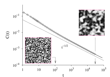
Figure 4: Temporal behavior of the concentration of particles for the A$+$B$\to 0$ model starting with randomly mixed A and B. The solid line is the result from the simulation using $16$ processors and the dots are from using a single processor. The $t^{-1/2}$ curve shows the asymptotic behavior. The two snapshots show the system at different times.

In Fig.4 we present the temporal behavior and also illustrate the segregation process forming regions with high concentration of A or B, which increase in size with time. Also we show how the global concentration, $C=N_{A}/L^{2}=N_{B}/L^{2}$, diminishes with time following the asymptotic power–law $C\sim t^{-\frac{1}{2}}$. The system size used is $L=8192$ and the parameters are $k=D=1$. We present two sets of data in Fig.4. The points correspond to a single processor simulation, and the solid line corresponds to a parallel simulation using $16$ processors. Both simulations start with identical random initial distribution of particles. It is noticeable that this initial distribution almost completely determines the following behavior of the system. The snapshots shown as insert in Fig.4 are from the parallel simulation. They are very similar to the ones obtained from the single processor simulation, which uses the same initial conditions but a different sequence of random numbers to simulate the dynamics. Moreover, in order to check quantitatively the agreement between spatial structures between the single and parallel simulations, we present in Fig.5 the radial correlation function. Again the points correspond to the single processor case and the solid line to the parallel case. A correlation length $r_{c}$ could be obtained by fitting these correlation functions with $\exp[-(r/r_{c})^{2}]$, which we show in Fig.5 by dashed lines. The obtained values of $r_{c}$ are plotted in the insert. This shows that the correlation length for this dynamic also follows a power–law $r_{c}\sim t^{\alpha}$. By numerical fitting we obtain $\alpha=0.5122\pm 0.012$. An analytical asymptotical solution for this correlation functions is given in kot1996 , $\exp(-r^{2}/4Dt)$ or $\exp[-c(r/\xi(t))^{2}]$. The previous value obtained for $\alpha$ means that the diffusion length $\xi(t)=\sqrt{Dt}$ define the scale of pattern formation for this reaction model.

Figure 5: The radial correlation function for the A$+$B$\to 0$ model The same times as the snapshots in Fig.4. The lines are the $16$ processor results and the dots the single processor results. The dashed lines are fits with $\exp[-(r/r_{c})^{2}]$. The respective values $r_{c}(t)$ are plotted in the insert.

The performance or speed up of the parallel algorithm for the A$+$B$\to 0$ model is shown in Fig.6, using different system sizes $L=256,512,1024,4096,8192$ and number of processors $P=1,2,4,8,16$. The simulated time for each computation was set to $t_{max}=500$. The speed was normalized to the speed of the single processor case. In the insert we can see the behavior of the single processor speed for each system sizes. The advantage of use a large number of processors increases when the system size increases, as we expect from the discussion in the previous section.

Figure 6: The speed of the simulation using $P$ processors normalized to the speed of one single processor for the A$+$B$\to 0$ model. Different system sizes $L=256,512,1024,4096,8192$ and number of processors $P=1,2,4,8,16$. In the insert the behavior of the speed of one single processor.

The second model used to test the parallel algorithm is a model for CO oxidation on Pt$(100)$ and Pt$(110)$ surfaces kuz1998 ; kor1998b ; kor1999 ; kuz1999 ; kor1999b . This system shows different types of kinetic oscillations. On Pt$(100)$ local, irregular oscillations occur in a wide parameter interval, whereas on Pt$(110)$ globally synchronized oscillations exist only in a very narrow parameter interval. Both surfaces exhibit an $\alpha\rightleftharpoons\beta$ surface reconstruction, where $\alpha$ denotes the hex or $1\times 2$ phase on Pt$(100)$ or Pt$(110)$, respectively. $\beta$ denotes the unreconstructed $1\times 1$ phase in both cases. Both surfaces have qualitatively quite similar properties with the exception of the dissociative adsorption of O₂. The ratio of the sticking coefficients of O₂ on the two phases is $s_{\alpha}:s_{\beta}\approx 0.5:1$ for Pt$(110)$ and $s_{\alpha}:s_{\beta}\approx 10^{-2}:1$ for Pt$(100)$ imb1995 . From the experiments imb1995 it is known that kinetic oscillations are closely connected with the $\alpha\rightleftharpoons\beta$ reconstruction of the Pt surfaces.

In the model kuz1998 ; kor1998b ; kor1999 ; kuz1999 ; kor1999b , CO is able to absorb onto a free surface site with rate constant $y$ and to desorb from the surface with rate constant $k$, independent of the surface phase to which the site belongs. O₂ adsorbs dissociatively onto two nearest neighbor sites with rate constant $(1-y)s_{\chi}$ with $\chi=\alpha$,$\beta$. In addition CO is able to diffuse via hopping onto a vacant nearest neighbor site with rate constant $D$. The CO$+$O reaction occurs with rate constant $R$, when CO and O are in nearest neighbor sites desorbing the reaction product CO₂. The $\alpha\rightleftharpoons\beta$ surface phase transition is modeled as a linear front propagation induced by the presence of CO in the border between phases with rate constant $V$. Consider two nearest neighbor surface sites in the state $\alpha\beta$. The transition $\alpha\beta\to\alpha\alpha$ ($\alpha\beta\to\beta\beta$) occurs if none (at least one) of these two sites is occupied by CO. Summarizing the above transition definitions written in the more usual form of reaction equations gives:

$$\mbox{CO(g)}+S^{\chi}\rightleftharpoons\mbox{CO(a)},$$

$$\mbox{O${}_{2}$(g)}+2S^{\alpha}\to 2\mbox{O(a)},$$

$$\mbox{O${}_{2}$(g)}+2S^{\beta}\to 2\mbox{O(a)},$$

$$\mbox{CO(a)}+S^{\chi}\to S^{\chi}+\mbox{CO(a)},$$

$$\mbox{CO(a)}+\mbox{O(a)}\to\mbox{CO${}_{2}$(g)}+2S^{\chi},$$

$$S^{\alpha}\rightleftharpoons S^{\beta},$$

where $S$ stands for a free adsorption site, $\chi$ stands for either $\alpha$ or $\beta$ and (a) or (g) for a particle adsorbed on the surface or in the gas phase, respectively. For additional details see ref. kuz1998 .

Amongst several successful results of this model, we can mention that it was one of the first microscopic models for CO oxidation on Pt including surface reconstruction, which is nowadays widely accepted as the key element in order to get oscillatory behavior. This model reproduce correctly oscillatory regimes for both surfaces Pt$(100)$ and Pt$(110)$, by changing only one parameter $s_{\alpha}$. The diffusion of CO is consider explicitly and could be applied to the fast diffusion regime without modification. With this model an alternative mechanism for global synchronization of oscillation has been suggested kor1999 , different from the traditional gas–phase coupling. This new mechanism is stochastic resonance, obtained by including a spontaneous nucleation of one surface phase in the other $\alpha\rightleftharpoons\beta$ at very low rates. One unique result reproducing experimental observations is the transition into chaotic behavior via the Feigenbaum route or period doubling kor1998b . It is also for this model that the compatibility of both microscopic simulations MC and CA has been study extensively kor1998 .

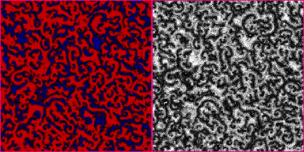
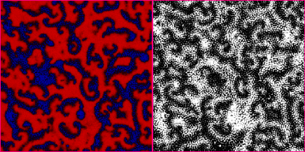
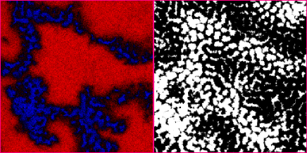
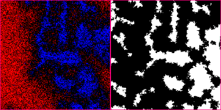
Figure 7: Sequence of snapshots of the model of CO oxidation on Pt$(110)$. The left part shows the chemical species: CO particles are dark–grey, O particles are light–grey, and empty sites are black. The right part shows the structure of the surface: $\alpha$ phase sites are black, and $\beta$ phase sites are white. The parameters are $L=8192$, $D=250$, and $V=1$, $y=0.494$, $k=0.1$, $R=D$. From top to bottom, we show sections from the upper–left corner with sizes $4096\times 4096$, $1024\times 1024$, $256\times 256$.

In Fig.7 we show snapshots from a simulation on Pt$(110)$ and a system size $L=8192$ using the parameter values, $D=250$, $V=1$, $y=0.494$, $k=0.1$, $R=D$. In the left part we plot the chemical species: CO particles are dark–grey, O particles are light–grey, and empty sites are black. The right part shows the structure of the surface: $\alpha$ phase sites are black, and $\beta$ phase sites are white. The pattern formation in this regime shows a spatio–temporal behavior, where a spiral dynamics is the dominant phenomena. It is interesting see the different structures at different spatial scales. For this purpose we include in Fig.7 sections from the upper–left corner with sizes $4096\times 4096$, $1024\times 1024$, $256\times 256$, from top to bottom. This sequence shows that the spiral dynamics occurs on a slowly varying island structure of sizes of the order of $\sqrt{D/V}$. The fact that we can see both mesoscopic and microscopic pattern formation is a quite interesting feature of the model, which has some experimental evidence win1997 ; vol1999 and has been studied theoretically in hil2002 by including lateral interactions between adsorbed particles. The model used here is simpler, because does not need that consideration in order to obtain nanostructures.

Figure 8: The same as Fig.6, but for the model of CO oxidation on Pt$(110)$.

In Fig.8 we analyze the speed up of the parallel algorithm of this realistic model. We use system sizes, $L=256,512,1024,4096,8192$ and number of nodes $P=1,2,4,8,16$. The simulated time for each computation was also set to $t_{max}=500$. Here we can see that the speed up of the parallel algorithm is good even for small system sizes. This is because the amount of computing in each node for this model is larger than for the A$+$B$\to 0$ model, while the amount of communication data is the same in both models.

V Conclusions

In this paper we present a tool to obtain scaling laws connecting experimental system sizes and diffusion coefficients to standard values in microscopic MC simulations. By using a CA equivalent to MC simulation we provide an efficient parallelization algorithm. We have explained in detail how to implement the parallelization. The speed up of the algorithm is almost ideal and it is much better for larger system sizes and more complex models. A full description and analysis of the scaling laws for the second model used here is in preparation sal2002 .

- (1) M.I. Rabinovich, A.B. Ezersky, P.D. Weidman, The dynamics of patterns. Word Scientific, Singapure, (2000).
- (2) R. Imbihl, G. Ertl, Chem. Rev. 95, 697 (1995).
- (3) D. Walgraef, Spatio–Temporal Pattern Formation: With Examples from Physics, Chemistry, and Materials Science. Springer Verlag, Berlin, (1997).
- (4) J. Wintterlin, Chaos, 12, 108 (2002).
- (5) N.G. van Kampen Stochastic Processes in Physics and Chemistry. North–Holland, Amsterdam, (1981).
- (6) D.T. Gillespie, J. Phys. Chem. 81, 2340 (1977).
- (7) A.P.J. Jansen, Comp. Phys. Comm. 86, 1 (1995).
- (8) J.J. Lukkien, J.P.L Segers, P.A.J. Hilbers, R.J. Gelten, A.P.J. Jansen, Phys. Rev. E 58, 2598 (1998).
- (9) G. Zvejnieks and V.N. Kuzovkov, Phys. Rev. E, 65, 051104 (2001).
- (10) J. Wintterlin, S. Völkening, T.V.W. Janssens, T. Zambelli, G. Ertl, Science 278, 1931 (1997).
- (11) S. Völkening, K. Bedürftig, K. Jacobi, J. Wintterlin, G. Ertl, Phys. Rev. Lett. 83, 2672 (1999).
- (12) T. Toffoli, N. Margolus, Cellular Automata Machines. MIT Press, Massachusetts, (1987).
- (13) J.R. Weimar, Simulation with Cellular Automata. Logos Verlag, Berlin (1997).
- (14) O. Kortlüke, J. Phys. A 31, 9185 (1998).
- (15) Cellular automata; From modeling to applications. Special Issue, Parallel Computing 27 (2001).
- (16) J.R. Weimar, Parallel Computing 27, 601 (2001).
- (17) B. Chopard, M. Droz, J. Phys. A 21, 205 (1988).
- (18) B. Chopard, M. Droz, J. Stat. Phys. 64, 859 (1991).
- (19) J. Mai, W. von Niessen, Phys. Rev. A 44, R6165 (1991).
- (20) J. Mai, W. von Niessen, Chem. Phys. 165, 57 (1992).
- (21) J. Mai, W. von Niessen, Chem. Phys. 165, 65 (1992).
- (22) J. Mai, W. von Niessen, J. Chem. Phys. 98, 2032 (1993).
- (23) By using processors and a system size the total interface between blocks is for the squares and for the strips . However, due to the cyclic tiling sequence shown in Fig.3 we reduce the amount of data to be send in half for the strips case. The ratio of data to be sent between squares and strips then is: .
- (24) D.E. Knuth, The art of computer programming, Vol.2: Seminumerical algorithms. Addison–Wesley, Amsterdam, (1998).
- (25) V.N. Kuzovkov, O. Kortlüke, W. von Niessen, J. Chem. Phys 108, 5571 (1998).
- (26) O. Kortlüke, V.N. Kuzovkov, W. von Niessen, Phys. Rev. Lett. 81, 2164 (1998).
- (27) O. Kortlüke, V.N. Kuzovkov, W. von Niessen, Phys. Rev. Lett. 83, 3089 (1999).
- (28) V.N. Kuzovkov, O. Kortlüke, W. von Niessen, Phys. Rev. Lett. 83, 1636 (1999).
- (29) O. Kortlüke, V.N. Kuzovkov, W. von Niessen, J. Chem. Phys 110, 11523 (1999).
- (30) A.A. Ovchinnikov, Ya.B. Zeldovich, Chem. Phys. 28, 215 (1978).
- (31) V.N. Kuzovkov, E.A. Kotomin Rep. Prog. Phys. 51, 1479 (1988).
- (32) E.A. Kotomin, V.N. Kuzovkov, Modern Aspects of Diffusion-Controlled Reactions: Cooperative Phenomena in Bimolecular Processes. North–Holland, Amsterdam, Vol.34, (1996).
- (33) V. Privman, Nonequilibrium Statistical Mechanics in One Dimension. Universitary Press, Cambridge (1997).
- (34) J. Marro, R. Dickman, Nonequilibrium phase transitions in lattice models. Universitary Press, Cambridge (1999).
- (35) P. Argyrakis, S.F. Burlatsky, E. Clement, G. Oshanin, Phys. Rev. E. 63, 021110 (2001).
- (36) B.P. Lee, J. Cardy, J. Stat. Phys. 80, 971 (1995).
- (37) D. Toussaint, F. Wilczek, J. Chem. Phys. 78, 2642 (1983).
- (38) M. Hildebrand, Chaos, 12, 144 (2002).
- (39) R. Salazar, A.P.J. Jansen, V.N. Kuzovkov Preprint.