Termination of Reentry in an Inhomogeneous Ring of Model Cardiac Cells

Abstract

Reentrant waves propagating in a ring or annulus of excitable media are a model of the basic mechanism underlying a major class of irregular cardiac rhythms known as anatomical reentry. Such reentrant waves are terminated by rapid electrical stimulation (pacing) from an implantable device. Because the mechanisms of such termination are poorly understood, we study pacing of anatomical reentry in a one-dimensional ring of model cardiac cells. For realistic off-circuit pacing, our model-independent results suggest that circuit inhomogeneities, and the electrophysiological dynamical changes they introduce, may be essential for terminating reentry in some cases.

Reentrant tachycardias, abnormally rapid excitations of the heart that result from an impulse that rotates around an inexcitable obstacle (“anatomical reentry”) [1] or within a region of cardiac tissue that is excitable in its entirety (“functional reentry”) [2, 3], may be fatal when they arise in the heart’s ventricles. Trains of local electrical stimuli are widely used to restore normal wave propagation in the heart during tachycardia. Such “antitachycardia pacing” is not always successful and may inadvertently cause tolerated tachycardias to degenerate to more rapid and threatening spatiotemporally irregular cardiac activity such as ventricular fibrillation [4]. The underlying mechanisms governing the success or failure of antitachycardia pacing algorithms are not yet clear. Understanding these mechanisms is essential, as a better knowledge of the processes involved in the suppression of ventricular tachycardia (VT) through such pacing might aid in the design of more effective therapies.

Several factors influence the ability of rapid pacing to interact with VT. The most prominent are[5]: (a) VT rate (for anatomical reentry this is determined by the length of the VT circuit and impulse conduction velocity around the obstacle), (b) the refractory period (i.e., the duration of time following excitation during which cardiac tissue cannot be re-excited) at the pacing site and in the VT circuit, (c) the conduction time from the pacing site to the VT circuit, and (d) the duration of the excitable gap (the region of excitable tissue in the VT circuit between the front and refractory tail of the reentrant wave [6]). A single stimulus is rarely sufficient to satisfy the large number of conditions for successfully terminating reentry. Therefore, in practice, multiple stimuli are often used – where the earlier stimuli are believed to “peel back” refractoriness to allow the subsequent stimuli to enter the circuit earlier than was possible with only a single stimulus [5].

The dynamics of pacing termination of one-dimensional reentry has been investigated in a number of studies [2, 7, 8, 9, 10], but most of these were concerned exclusively with homogeneous ring of cardiac cells. The termination of reentry in such a geometry (which is effectively that of the reentry circuit immediately surrounding an anatomical obstacle) occurs in the following manner. Each stimulus splits into two branches that travel in opposite directions around the reentry circuit. The retrograde branch (proceeding opposite to the direction of the existing reentrant wave) ultimately collides with the reentrant wave, causing mutual annihilation. The anterograde branch (proceeding in the same direction as the reentrant wave) can, depending on the timing of the stimulation, lead to resetting, where the anterograde wave becomes a new reentrant wave, or termination of reentry, where the anterograde wave is blocked by the refractory tail of the original reentrant wave. From continuity arguments, it can be shown that there exists a range of stimuli phases and amplitudes that leads to successful reentry termination [7]. Unfortunately, the argument is essentially applicable only to a 1D ring – the process is crucially dependent on the fact that the pacing site is on the reentry circuit itself. However, in reality, the location of the reentry circuit is typically not known when an electrical pacing device is implanted, and, it is unlikely that the pacing site will be so fortuitously located.

In this study, we examine the dynamics of pacing from a site located some distance away from the reentry circuit. Such off-circuit pacing introduces the realistic propagation of the stimulus from the pacing site to the reentry circuit. Because reentrant waves propagate outwardly from, in addition to around, the circuit, the stimulus will be blocked before it reaches the circuit under most circumstances. Multiple stimuli are necessary to “peel back” refractory tissue incrementally until one successfully arrives at the reentry circuit [5]. Further, once a stimulus does reach the circuit, its anterograde branch must be blocked by the refractory tail of the reentrant wave, or resetting will occur and termination will fail. However, as outlined below, this is extremely unlikely to happen in a homogeneous medium.

Let us consider a reentrant circuit as a 1D ring of length $L$ with separate entrance and exit sidebranches (Fig. 1). This arrangement is an abstraction of the spatial geometry involved in anatomical reentry [5]. Further, let the pacing site be located on the entrance sidebranch at a distance $z$ from the circuit. We use the entrance sidebranch as the point of spatial origin ($x=0$) to define the location of the wave on the ring. The conduction velocity and refractory period at a location a distance $x$ away (in the clockwise direction) from the origin are denoted by $c(x)$ and $r(x)$, respectively.

For a homogeneous medium, $c(x)=c$, $r(x)=r$ ($c,r$ are constants). Therefore, the length of the region in the ring which is refractory at a given instant is $l=cr$. For sustained reentry to occur, an excitable gap must exist (i.e., $L>c~{}r$). We assume that restitution effects (i.e., the variation of the action potential duration as a function of the recovery time) can be neglected. Further, the circuit length $L$ is considered to be large enough so that the reentrant activity is simply periodic. For convenience, associate $t=0$ with the time when the reentrant wavefront is at $x=0$ (i.e., the entrance sidebranch) [Fig. 1(a)]. Let us assume that a stimulus is applied at $t=0$. This stimulus will collide with the branch of the reentrant wave propagating out through the entrance sidebranch at $t=z/2c$ [Fig. 1(b)]. The pacing site will recover at $t=r$ and if another stimulus is applied immediately it will reach the reentry circuit at $t=r+(z/c)$ [Fig. 1(c)]. By this time the refractory tail of the reentrant wave will be at a distance $x=z$ away from the entrance sidebranch and the anterograde branch of the stimulus will not be blocked. Thus, when $z>0$, it is impossible for the stimulus to catch up to the refractory tail in a homogeneous medium. This results in resetting of the reentrant wave rather than its termination.

Note that, if the first stimulus is given at a time $t<-z/c$, it reaches the reentry circuit before the arrival of the reentrant wave. As a result, the retrograde branch collides with the oncoming reentrant wave, while the anterograde branch proceeds to become the reset reentrant wave. Even in the very special circumstance that the reentrant wave reaches the entrance sidebranch exactly at the same instant that the stimulus reaches the circuit, the two colliding waves allow propagation to continue along the reentrant circuit through local depolarization at the collision site. As a result, pacing termination seems all but impossible in a homogeneous reentry circuit.

The situation changes, however, if an inhomogeneity (e.g., a zone of slow conduction) exists in the circuit [Fig. 1(d)]. In this case, the above argument no longer holds because the inhomogeneity alters the electrophysiological dynamics (notably refractory period) of the excitation waves. As a result, stimuli may arrive at the circuit from the pacing site and encounter a region that is still refractory. This leads to successful block of the anterograde branch of the stimulus, while the retrograde branch annihilates the reentrant wave (as in the homogeneous case), resulting in successful termination.

The following simulation results also support the conclusion that the existence of inhomogeneity in the reentry circuit is essential for pacing termination of VT. We assume that the cardiac impulse propagates in a continuous one-dimensional ring of tissue (ignoring the microscopic cell structure) with ring length $L$, representing a closed pathway of circus movement around an anatomical obstacle (e.g., scar tissue). The propagation is described by the partial differential equation:

$${\partial V}/{\partial t}=-I_{ion}/C_{m}+D{\nabla}^{2}V,$$ (1)

where $V$ (mV) is the membrane potential, $C_{m}$ = 1 $\mu$F cm^-2 is the membrane capacitance, $D$ (cm² s^-1) is the diffusion constant and $I_{ion}$ ($\mu$A cm^-2) is the cellular transmembrane ionic current density. We used the Luo-Rudy I action potential model [11], in which $I_{ion}$ = $I_{Na}$ + $I_{si}$ + $I_{K}$ + $I_{K1}$ + $I_{Kp}$ + $I_{b}$. $I_{Na}=G_{Na}m^{3}hj(V-E_{Na})$ is the fast inward Na⁺ current, $I_{si}=G_{si}df(V-E_{si})$ is the slow inward current, $I_{K}=G_{K}xx_{i}(V-E_{K})$ is the slow outward time-dependent K⁺ current, $I_{K1}=G_{K1}K1_{\infty}(V-E_{K1})$ is the time-independent K⁺ current, $I_{Kp}=0.0183K_{p}(V-E_{Kp})$ is the plateau K⁺ current, and $I_{b}=0.03921(V+59.87)$ is the total background current. $m$, $h$, $j$, $d$, $f$, $x$ and $x_{i}$ are the gating variables satisfying differential equations of the type: $dy/dt=(y_{\infty}-y)/{\tau}_{y}$, where $y_{\infty}$ and ${\tau}_{y}$ are dimensionless quantities which are functions solely of $V$. The external K⁺ concentration is set to be $[$K$]_{0}$ = 5.4mM, while the intracellular Ca²⁺ concentration obeys $d[{\rm Ca}]_{i}/dt=-10^{-4}I_{si}+0.07(10^{-4}-[{\rm Ca}]_{i})$. The details of the expressions and the values used for the constants can be found in Ref.[11]. We solve the model by using a forward-Euler integration scheme. We discretize the system on a grid of points in space with spacing $\delta x$ = 0.01 cm (which is comparable to the length of an actual cardiac cell) and use the standard three-point difference stencil for the 1-D Laplacian. The spatial grid consists of a linear lattice with $L$ points; in this study we have used $L=2500$. The integration time step used in our simulations is $\delta t$ = 0.005 ms. The initial condition is a stimulated wave at some point in the medium with transient conduction block on one side to permit wavefront propagation in a single direction only. Extrastimuli are introduced from a pacing site.

To understand the process of inhomogeneity-mediated termination we introduced a zone of slow conduction in the ring. Slow conduction has been observed in cardiac tissue under experimental ischemic conditions (lack of oxygen to the tissue) [12] and the conduction velocity in affected regions is often as low as $10\%$ of the normal propagation speed in the ventricle [13]. This phenomenon can be reasonably attributed to a high degree of cellular uncoupling [14], as demonstrated by model simulations [15]. In our model, slow conduction was implemented by varying the diffusion constant $D^{\prime}$ from the value of $D$ used for the remainder of the ring. The length and diffusion constant($D^{\prime}$) of the zone were varied to examine their effect on the propagation of the anterograde branch of the stimulus. We found that varying the length of the zone of slow conduction (specifically, between 1.5 mm and 25 mm) had no qualitative effect on the results. For the simulation results reported below we used $D$ = 0.556 cm²/s and $D^{\prime}$ = 0.061 cm²/s, corresponding to conduction velocities $c\simeq$ 47 cm/s and $c^{\prime}\simeq$ 12 cm/s, respectively, which are consistent with the values observed in human ventricles [13, 16].

The reentrant wave activates the point in the ring (proximal to the zone of slow conduction) chosen to be the origin ($x=0$), where the stimulus enters the ring, at time $t=T_{0}$. At time $t=T_{1}$, an activation wave is initiated through stimulation at $x=0$. If this first stimulus is unable to terminate the reentry, a second stimulus is applied at $t=T_{2}$, again at $x=0$. Note that, the first stimulus is always able to terminate the reentry if it is applied when the region on one side of it is still refractory – leading to unidirectional propagation. This is identical to the mechanism studied previously for terminating reentry by pacing within a 1D ring [7]. However, in this study we are interested in the effect of pacing from a site away from the reentry circuit. In that case, it is generally not possible for the first stimulus to arrive at the reentry circuit exactly at the refractory end of the reentrant wave (as discussed above). Therefore, we have used values of $T_{1}$ for which the first stimulus can give rise to both the anterograde, as well as the retrograde branches, and only consider reentry termination through block of the anterograde branch of the stimulated wave in the zone of slow conduction.

Fig. 2 (top) shows an instance of successful termination of the reentrant wave where the anterograde branch of the stimulus applied at $T_{1}=1146.22$ ms ($T_{1}-T_{0}=428.00$ ms) is blocked at the boundary of the zone of slow conduction (at time $t\simeq 1253$ ms, $x=50$ mm). Fig. 2 (bottom) shows a magnified view of the region at which conduction block occurs. The region immediately within the zone of slow conduction shows depolarization but not an action potential (i.e., the excitation is subthreshold), while the region just preceding the inhomogeneity has successively decreasing action potential durations. The peak membrane potential attained during this subthreshold depolarization sharply decreases with increasing depth into the inhomogeneity so that, at a distance of 0.5 mm from the boundary inside the zone of slow conduction, no appreciable change is observed in the membrane potential $V$. For the same simulation parameters as Fig. 2, a single stimulus applied at $T_{1}-T_{0}>428.63$ ms is not blocked at the inhomogeneity, and a second stimulus needs to be applied at time $T_{2}$ to terminate reentry.

Different values of coupling interval ($T_{1}-T_{0}$) and pacing interval ($T_{2}-T_{1}$) were used to find which parameters led to block of the anterograde wave. Fig. 3 is a parameter space diagram which shows the different parameter regimes where termination was achieved.

The conduction block of the anterograde branch of the stimulated wave is due to a dynamical effect linked to a local increase of the refractory period at the boundary of the zone of slow conduction in the reentrant circuit. To obtain an idea about the variation of refractory period around the inhomogeneity, we measure the closely related quantity, action potential duration (APD). Fig. 4 shows the variation of the APD as the reentrant wave propagates across the ring. The APD of an activation wave was approximated as the time-interval between successive crossing of $-60$ mV by the transmembrane potential $V$ [17]. As the wave crosses the boundary into the region of slow conduction, the APD increases sharply. Within this region, however, the APD again decreases sharply. Away from the boundaries, in the interior of the region of slow conduction, the APD remains constant until the wave crosses over into the region of faster conduction again, with a corresponding sharp decrease followed by a sharp increase of the APD, around the boundary. This result is consistent with the observation by Keener [18] that non-uniform diffusion has a large effect on the refractory period in discrete systems.

However, the APD lengthening alone cannot explain the conduction block. Fig. 4 shows that the maximum APD, at the boundary of the inhomogeneity, is $\sim 345$ ms, yet conduction failed for a coupling interval of 428.00 ms. The blocking of such a wave (i.e., one that is initiated at a coupling interval that is significantly longer than the previous APD) implies that APD actually underestimates the effective refractory period. While it is believed that such “postrepolarization refractoriness” does not occur in homogeneous tissue, it has been observed experimentally for discontinuous propagation of excitation [19, 20]. Postrepolarization refractoriness is caused by residual repolarizing ionic current that persists long after the transmembrane potential has returned almost to its quiescent value. As seen in Fig. 5, this has occurred in our system – at the time when the electrotonic current of the stimulated wave begins entering the inhomogeneity, the ionic current has not fully recovered from the previous wave, and is actually working against the electrotonic current ($I_{ion}>0$). If the stimulated wave is early enough, this ionic current mediated postrepolarization refractoriness is enough to prevent the electrotonic current from depolarizing the zone of slow conduction.

This prolongation of the refractory period at the border of the inhomogeneity is the underlying cause of the conduction block leading to successful termination of reentry, as can be seen in Fig. 6. Here, we compare the behavior at the inhomogeneity boundary when the wave is blocked (CI = 428.00 ms) with the case when the wave does propagate through the inhomogeneity (CI = 428.64 ms). As already mentioned, in the case of block, the depolarization of the region immediately inside the zone of slow conduction is not sufficient to generate an action potential. Instead, the electrotonic current increases the transmembrane potential $V$ to $\sim-55$ mV and then slowly decays back to the resting state. On the other hand, if the stimulation is applied only 0.64 ms later, $V$ (as in the earlier case) rises to $\sim-55$ mV and then after a short delay ($\sim 8$ ms) exhibits an action potential. This illustrates that in the earlier case the region had not yet recovered fully when the stimulation had arrived.

Fig. 7 shows in detail how the difference in diffusion constant in the inhomogeneity leads to conduction block [21]. In the region with normal diffusion constant [Fig. 7 (a)], the initial stimulation for a region to exhibit an action potential is provided by current arriving from a neighboring excited region. This spatial “electrotonic” current $I_{spat}=C_{m}D\nabla^{2}V$ is communicated through gap junctions which connect neighboring cardiac cells. As soon as the “upstream” neighboring region is excited with a corresponding increase in potential $V$, the difference in membrane potentials causes an electrotonic current to flow into the region under consideration (positive deflection in $I_{spat}$). This causes the local potential to rise and subsequently, an outward current to the “downstream” neighboring non-excited region is initiated (negative deflection in $I_{spat}$). Thus, the initial net current flow into the region is quickly balanced and is followed, for a short time, by a net current flow out of the region, until the net current $I_{spat}$ becomes zero as the membrane potential $V$ reaches its peak value. The change in $V$ due to $I_{spat}$ initiates changes in the local ionic current $I_{ion}$. This initially shows a small positive hump, followed by a large negative dip (the inward excitatory rush of ionic current), which then again sharply rises to a small positive value (repolarizing current) and gradually goes to zero. The net effect of the changes in $I_{spat}$ and $I_{ion}$ on the local membrane potential $V$ is reflected in the curve for $\partial V/\partial t=D\nabla^{2}V-(I_{ion}/C_{m})$. This shows a rapid increase to a large positive value and then a decrease to a very small negative value as the membrane potential $V$ reaches its peak value followed by a slight decrease to the plateau phase value of the action potential.

At the boundary of the inhomogeneity, however, the current $I_{spat}$ is reduced drastically because of the low value of the diffusion constant $D^{\prime}$ at the inhomogeneity [Figs. 6(b) and 7(b)]. Physically, this means that the net current flow into the cell immediately inside the region of slow conduction is much lower than in the normal tissue. This results in a slower than normal depolarization of the region within the inhomogeneity. Because the region is not yet fully recovered, this reduced electrotonic current is not sufficient to depolarize the membrane beyond the excitation threshold. Therefore, the depolarization is not accompanied by the changes in ionic current dynamics needed to generate an action potential in the tissue [Fig. 6(c)]. The resulting $\partial V/\partial t$ curve therefore shows no significant positive peak. Hence, the initial rise in $V$ is then followed by a decline back to the resting potential value as is reflected in the curve for $\partial V/\partial t$ in Fig. 6(d).

When the stimulation is given after a longer coupling interval ($T_{1}-T_{0}$) , i.e., after the cells in the inhomogeneous region have recovered more fully, a different sequence of events occurs. As in the case shown in Fig. 7(b), the depolarization of the region immediately inside the zone of slow conduction is extremely slow because of the reduced electrotonic current $I_{spat}$. However, because the tissue has had more time to recover, the electrotonic current depolarizes the membrane potential beyond the threshold and the ionic current mechanism responsible for generating the action potential is initiated (as illustrated by the broken curves in Fig 6). As a result, the excitation is not blocked but propagates through the inhomogeneity, although with a slower conduction velocity than normal because of the longer time required for the cells to be depolarized beyond the excitation threshold.

To ensure that these results are not model dependent, especially on the details of ionic currents, we also looked at a modified Fitzhugh-Nagumo type excitable media model of ventricular activation proposed by Panfilov [22]. The details about the simulation of the Panfilov model are identical to those given in Refs. [23, 24]. This two-variable model lacks any description of ionic currents and does not exhibit either the restitution or dispersion property of cardiac tissue. As expected, such differences resulted in quantitative changes in termination requirements (e.g., the parameter regions at which termination occurs for the Panfilov model are different from those shown in Fig. 3 for the Luo-Rudy model). Nevertheless, despite quantitative differences, these fundamentally different models shared the requirement of an inhomogeneity for termination, thereby supporting the model independence of our findings.

There are some limitations of our study. The most significant one is the use of a 1D model. However, our preliminary studies on pacing in a 2D excitable media model of anatomical reentry [24] show similar results. We have also assumed the heart to be a monodomain rather than a bidomain (which has separate equations for intracellular and extracellular space). We believe this simplification to be justified for the low antitachycardia pacing stimulus amplitude. We have used a higher degree of cellular uncoupling to simulate ischemic tissue where slow conduction occurs. However, there are other ways of simulating ischemia [25], e.g., by increasing the external K⁺ ion concentration [26]. But this is transient and does not provide a chronic substrate for inducing irregular cardiac activity. Also, there are other types of inhomogeneity in addition to ischemic tissue. For example, existence of a region having longer refractory period will lead to the development of patches of refractory zones in the wake of the reentrant wave. If the anterograde branch of the stimulus arrives at such a zone before it has fully recovered, it will be blocked [1].

Despite these limitations, the results presented here offer insight into pacing termination of anatomical reentry in the ventricle. We have developed general (i.e., model independent) mathematical arguments, supported by simulations, that circuit inhomogeneities are required for successful termination of anatomical-reentry VT when stimulation occurs off the circuit (as is typical in reality). Thus, considering the critical role of such inhomogeneities may lead to more effective pacing algorithms.

We thank Kenneth M. Stein and Bruce B. Lerman for helpful discussions. This work was supported by the American Heart Association (#0030028N).

FIGURES

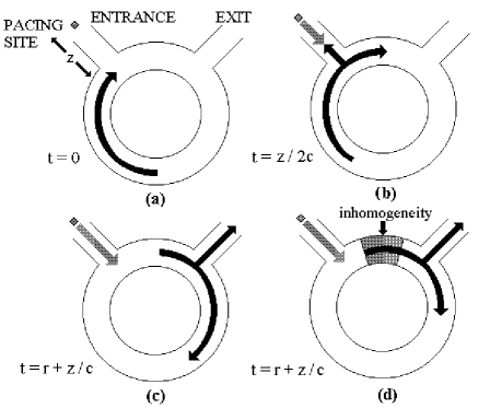
FIG. 1.: Schematic diagram of reentry in a 1D ring illustrating the necessity of a region of inhomogeneity for successful termination of reentry by pacing. At $t=0$ the reentrant wave reaches the entrance sidebranch (a). At $t=z/2c$ the reentrant wave propagating through the sidebranch and the first stimulus mutually annihilate each other (b). At $t=r+(z/c)$ the second stimulus reaches the reentry circuit by which time the refractory tail is a distance $z$ away from the sidebranch (c). The presence of a region of inhomogeneity in the ring makes it possible that the anterograde branch of the second stimulus will encounter a refractory region behind the reentrant wave (d).

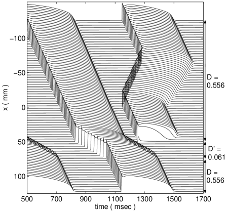
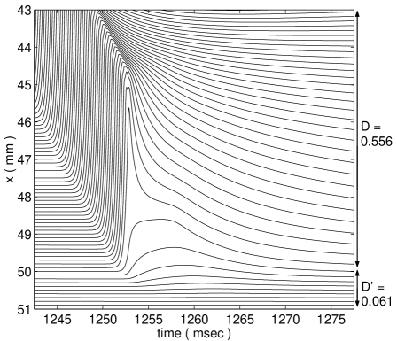
FIG. 2.: (top) Plot of the membrane potential, $V$, showing spatiotemporal propagation of a reentrant wave in a Luo-Rudy ring of length 250 mm, successfully terminated by pacing with a single stimulus. The zone of slow conduction is between $x$ = 50 mm and $x$ = 75 mm. In this region the diffusion constant changes from $D$ = 0.556 to $D^{\prime}$ = 0.061 cm²/s with an infinite gradient at the boundaries. The reentrant wave activates the site at $x$ = 0 mm at $T_{0}$ = 718.22 ms. The stimulus is applied at $x=0$ mm at $T_{1}$ = 1146.22 ms (coupling interval = 428.00 ms). (bottom) Magnification of the above plot for the region between $x=43$ mm and $x=51$ mm and the time interval $1242.50\leq t\leq 1277.50$ ms. Note that, inside the inhomogeneity, no action potential is generated.

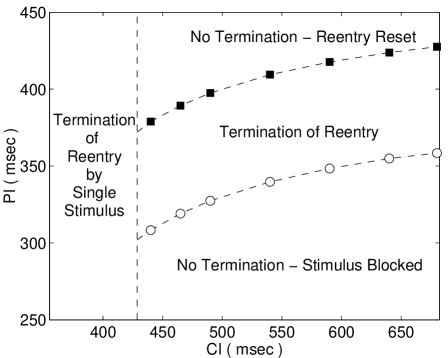
FIG. 3.: Parameter space diagram of coupling interval (CI) and pacing interval (PI) at which termination occurs in the 1D Luo-Rudy ring of length 250 mm with a zone of slow conduction between $x$ = 50 mm and 75 mm ($D$ = 0.556 cm²/s, $D^{\prime}$ = 0.061 cm²/s). The VT period around the ring is 692.46 ms. The line connecting the circles represents the critical pacing interval value below which the second stimulus gets blocked by the refractory tail of the first stimulus. The region between the circles and squares represents the regime in which the second stimulus is blocked in the anterograde direction in the zone of slow conduction (leading to successful termination) for a boundary with infinite gradient. For longer PI (the region above the squares), the second stimulus propagates through the inhomogeneity and only resets the reentrant wave. Note that the APD of the reentrant wave at $x$ = 0 is approximately 340.6 ms. For CI $<355.29$ ms, the first stimulus is blocked at $x=0$, while for CI $>428.63$ ms, the anterograde branch of the first stimulus is not blocked at the zone of slow conduction (leading to resetting of the reentrant wave). For intermediate values of CI (i.e., between $355.29-428.63$ ms), the first stimulus is able to successfully terminate reentry.

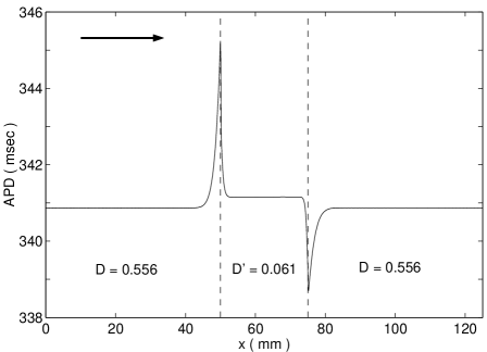
FIG. 4.: Variation of the action potential duration (APD) for the reentrant wave as it proceeds from $x$ = 0 to $x$ = 125 mm in the ring. The arrow indicates the direction of wave propagation. The dashed lines between $x$ = 50 mm and 75 mm enclose the region where the diffusion constant changes from $D$ = 0.556 to $D^{\prime}$ = 0.061 cm²/s with an infinite gradient at the boundaries.

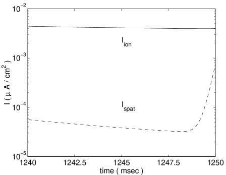
FIG. 5.: The ionic current $I_{ion}$ (solid curve) and the spatial electrotonic current $I_{spat}=C_{m}D\nabla^{2}V$ (broken curve) at $x=50$ mm (the boundary of the inhomogeneity). Note that, initially, the latter is two orders of magnitude smaller than the former. At $t\simeq 1248.5$ ms, $I_{spat}$ begins to increase due to current inflow from the upstream excited neighboring region. The high value of $I_{ion}$ throughout this time indicates that the boundary of the inhomogeneity has not yet recovered from the passage of the previous wave by the time the next stimulated wave arrives.

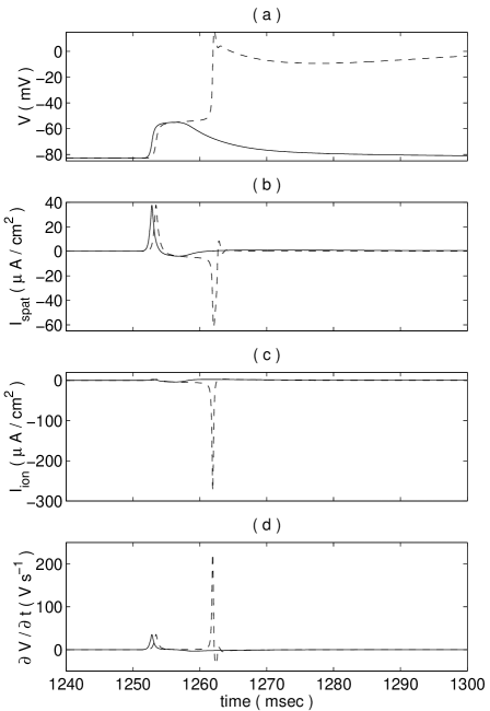
FIG. 6.: The (a) transmembrane potential $V$, (b) the spatial (electrotonic) current $I_{spat}=C_{m}D\nabla^{2}V$, (c) the ionic current $I_{ion}$, and (d) the rate of change of transmembrane potential $\partial V/\partial t=D\nabla^{2}V-(I_{ion}/C_{m})$, at $x=50$ mm for coupling intervals CI = 428.00 ms (solid curves) and 428.64 ms (broken curves) [$D$ = 0.556 cm²/s, $D^{\prime}$ = 0.061 cm²/s]. In the former case, the initial depolarization is insufficient to generate an action potential and the excitation wavefront is blocked. In the latter case, the region has recovered sufficiently so that the stimulation is able to generate an action potential and the wave propagates through the inhomogeneity.

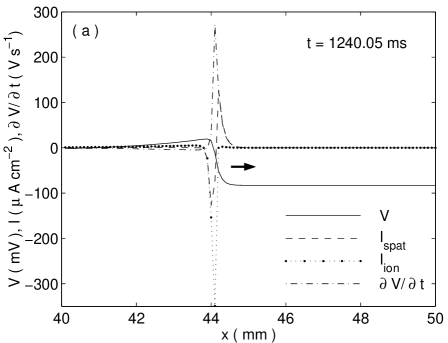
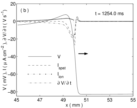
FIG. 7.: The spatial variation of transmembrane potential $V$, the spatial current $I_{spat}=C_{m}D\nabla^{2}V$, the ionic current $I_{ion}$, and the rate of change of transmembrane potential $\partial V/\partial t=D\nabla^{2}V-(I_{ion}/C_{m})$, in (a) a homogeneous region of tissue (at $t=1240.05$ ms) and (b) at the border of slow conduction (at $t=1254.00$ ms). The zone of slow conduction is between $x=50$ mm and $x=75$ mm ($D$ = 0.556 cm²/s, $D^{\prime}$ = 0.061 cm²/s) and the coupling interval is 428.00 ms. In (a) the excitation wavefront propagates normally, while in (b) the wavefront is blocked at the boundary of the inhomogeneity. The arrows indicate the direction of propagation of the wavefront.

REFERENCES

- [1] J. A. Abildskov and R. L. Lux, J. Electrocardiology 28, 107 (1995).
- [2] Y. Rudy, J. Cardiovasc. Electrophys. 6, 294 (1995).
- [3] J. M. Davidenko, R. Salomonsz, A. M. Pertsov, W. T. Baxter and J. Jalife, Circ. Res. 77, 1166 (1995).
- [4] M. E. Rosenthal and M. E. Josephson, Circulation 82, 1889 (1990).
- [5] M. E. Josephson, Clinical Cardiac Electrophysiology: Techniques and Interpretation, 2nd ed. (Lea Febiger, Philadelphia, 1993).
- [6] H. Fei, M. S. Hanna and L. H. Frame, Circ. 94, 2268 (1996).
- [7] L. Glass and M. E. Josephson, Phys. Rev. Lett. 75, 2059 (1995).
- [8] T. Nomura and L. Glass, Phys. Rev. E 53, 6353 (1996).
- [9] Z. Qu, J. N. Weiss and A. Garfinkel, Phys. Rev. Lett. 78, 1387 (1997).
- [10] A. Vinet and F. A. Roberge, Ann. Biomed. Eng. 22, 568 (1994).
- [11] C. H. Luo and Y. Rudy, Circ. Res. 68, 1501 (1991).
- [12] A. G. Kleber, C. B. Riegger and M. J. Janse, Circ. Res. 51, 271 (1987).
- [13] C. de Chillou, D. Lacroix, D. Klug, I. Magnin-Poull, C. Marquie, M. Messier, M. Andronache, C. Kouakam, N. Sadoul, J. Chen, E. Aliot and S. Kacet, Circ. 105 726 (2002).
- [14] S. Rohr, J. P. Kucera and A. G. Kleber, Circ. Res. 83, 781 (1998).
- [15] W. Quan and Y. Rudy, Circ. Res. 66, 367 (1990).
- [16] B. Surawicz, Electrophysiological Basis of ECG and Cardiac Arrhythmia (Lippincott Williams & Wilkins, Philadelphia, 1995), p. 76.
- [17] There are other methods of measuring APD which may make minor quantitative differences, but would not qualitatively change our findings.
- [18] J. Keener, J. Theo. Biol. 148, 49 (1991).
- [19] J. Jalife, C. Antzelevitch and G. K. Moe, Circ. 62, 912 (1983).
- [20] J. Jalife and M. Delmar, in Theory of Heart, edited by L. Glass, P. Hunter and A. McCulloch (Springer-Verlag, New York, 1991), p. 359.
- [21] For similar analysis of the qualitatively different dynamics of conduction block that occurs as a wave moves in the opposite direction (i.e., from a region of impaired coupling to normal tissue), see Y. Wang and Y. Rudy, Am. J. Physiol. Heart Circ. Physiol. 278, H 1019 (2000).
- [22] A. V. Panfilov and P. Hogeweg, Phys. Lett. A 176, 295 (1993); A. V. Panfilov, Chaos 8, 57 (1998).
- [23] S. Sinha, A. Pande and R. Pandit, Phys. Rev. Lett. 86, 3678 (2001).
- [24] S. Sinha and D. J. Christini, e-print nlin.CD/0107070; S. Sinha, K. M. Stein and D. J. Christini, Chaos 12, 893 (2002).
- [25] R. M. Shaw and Y. Rudy, Circ. Res. 80, 124 (1997).
- [26] F. Xie, Z. Qu, A. Garfinkel and J. N. Weiss, Am. J. Physiol. Heart Circ. Physiol. 280, H1667 (2001).