Fluctuations of wave functions about their classical average

Abstract

Quantum-classical correspondence for the average shape of eigenfunctions and the local spectral density of states are well-known facts. In this paper, the fluctuations that quantum mechanical wave functions present around the classical value are discussed. A simple random matrix model leads to a Gaussian distribution of the amplitudes. We compare this prediction with numerical calculations in chaotic models of coupled quartic oscillators. The expectation is broadly confirmed, but deviations due to scars are observed.

1 Introduction

At the turn of the century the study of the quantum manifestations of classical chaotic systems suffered a significant change. Before, the spectral statistics were amply discussed and it was shown that they follow the Random Matrix Theory (RMT) predictions  [1, 2]. The study of wave function properties, however, presents inherent difficulties arising from the dependence on the basis used, forcing either to specify one or to define basis independent quantities. Recent progress has been made in this respect in the study of average properties of eigenstates  [3, 4, 5] and of the significant statistical deviations from RMT  [6, 7]. Nevertheless, not much systematic work exists on the eigenfunction fluctuations in dynamical systems  [3]. In this work we shall contribute on the last subject.

In a recent paper [5] it was found that the suitably averaged matrix elements between the eigenfunctions (EF) of two arbitrary Hamiltonians $H_{0}$ and $H$ are well described in the semi-classical regime by a classical phase-space integral. Specifically, if we define $\phi_{\alpha}$, $E_{\alpha}^{(0)}$ to be the eigenfunctions and eigenvalues, respectively, of $H_{0}$ and $\psi_{i}$,$E_{i}$ those of $H$, one finds to a good approximation

$$\bigl{\langle}\left|\langle\phi_{\alpha}|\psi_{i}\rangle\right|^{2}\bigr{\rangle}=\frac{g(E_{\alpha}^{(0)},E_{i})}{\rho_{0}(E_{\alpha}^{(0)})},$$ (1)

where $g(\epsilon,E)$ is given by

$$g(\epsilon,E)=\int dp\,dq\,\delta\left(H_{0}(p,q)-\epsilon\right)\delta\left(H(p,q)-E\right),$$ (2)

which was called in reference [5] the classical eigenfunction for fixed $E$. Here $\rho_{0}(\epsilon)$ is the level density of $H_{0}$ calculated by means of Weyl’s formula. By the symmetry of equation (1), the local density of states(LDOS) can be calculated using the energy density of $H$ instead of $\rho_{0}(\epsilon)$ and maintaining fixed $\epsilon$ in equation (2). For the details, in particular about the way in which the l.h.s. of equation (1) must be averaged to obtain meaningful results, see reference  [5]. This study was exemplified by two systems of anharmonic oscillators in one dimension, one coupled and the other uncoupled. In the present letter, our interest is focused on the fluctuations of the quantum-mechanical wave functions around this classical limit in the chaotic case.

2 A Random-matrix model

In the usual description of chaotic systems by random matrices, the restrictions implied by equations (1) and (2) are not present. Rather, one attempts to deduce the average properties of the eigenfunctions given the structure of the random matrix ensemble in some particular basis. Instead, here we choose pairs of matrices $(H,H_{0})$ of size $N\times N$ in such a way that the condition

$$\left\langle\left|\langle\phi_{i}|\psi_{j}\rangle\right|^{2}\right\rangle=I_{i,j}$$ (3)

is always fulfilled, but the matrices are otherwise arbitrary. The angular brackets denote the average over the ensemble of matrix pairs and $I_{i,j}$ stand for any numbers given by outside constraints such as (1). Under these circumstances, we wish to determine the full distribution of the matrix elements $\langle\phi_{i}|\psi_{j}\rangle$. We then proceed to compare the predictions of this random matrix model with numerical results on models similar to that studied in [5].

To solve the above problem, we let ourselves be guided by the following considerations: the quantities we need to model, namely the $\langle\phi_{i}|\psi_{j}\rangle$, are nothing else than the matrix elements of an orthogonal matrix (a unitary one in the case where time-reversal invariance is broken, but this does not affect our conclusions). We therefore need a random matrix model for orthogonal matrices with prescribed expectation values for the intensities $I_{i,j}$. Note that, in the large $N$ limit, the Haar measure over the group of orthogonal matrices can be replaced, up to corrections of order $1/N$, by independent Gaussian distributions for all matrix elements $O_{i,j}$, all having a variance $1/N$. In other words, what we need is a random matrix model where the average intensity $I_{i,j}=\langle|O_{i,j})|^{2}\rangle$ is given. If $I_{i,j}\ll 1$, we can consider $1/I_{i,j}$ as an effective dimension and we expect to get the desired result, up to corrections of order $O(I_{i,j})$, if we replace the average by a simple Gaussian average. We may then, to this level of accuracy, take the $O_{i,j}$ as independent Gaussian variables with variances given by $I_{i,j}$.

Note that we postulate a distribution for orthogonal matrices with the correct values for $I_{i,j}$. We do not actually derive this distribution, but simply verify that it has all the required properties. If the classical wave function takes very large values and the eigenfunctions of $H$ do not have a sufficiently large number of components in the basis of $H_{0}$, it may happen that some $I_{i,j}\simeq 1$. Clearly, for these matrix elements the model will not apply; we shall see later that this happens near peaks or singularities in the classical wave function, but then we cannot really make any comparison with the specific system anyway. However, for the vast majority of matrix elements, we can expect that the amplitudes are Gaussian distributed and if we divide the amplitude $O_{i,j}$ by $\sqrt{I_{i,j}}$ we will find a standard Gaussian.

What deviations from the above predictions should we expect from a theoretical point of view? Clearly, scars [6] produce an excess of very small amplitudes, because a few exceptionally large amplitudes pick up more of the intensity than expected from the classical calculation. Would we also see the large amplitudes? Probably not in a statistical analysis against our model, because these will mainly occur in the region where the classical function is large and we will usually exclude this region: the condition $I_{i,j}\ll 1$ is violated there, unless we reach very high spectral densities, which is scarcely possible in a numerical experiment. In a real experiment, resolution might well make such a high-density region inaccessible also. If, on the other hand, localization occurs due to disorder or due to the fact that the system does not cover the whole phase space on the Heisenberg time scale [8], then we may indeed also see irregularities beyond the realm of very small amplitudes.

However, all deviations mentioned above should only be important if one of the Hamiltonians, say $H_{0}$, is integrable in the classical limit. If both are chaotic, and we exclude situations in which the two Hamiltonians are, in some sense, closely related, we can expect not to see any effect of the scars in the amplitudes. The reason for this can be understood in terms of the traditional picture due to Berry [9] of the eigenfunctions in phase space: For a chaotic Hamiltonian, they are expected to cover phase space essentially in a uniform way, up to rather small concentrations on periodic orbits. In integrable systems, on the other hand, eigenfunctions are localized on well-defined tori, with only half the dimension of the full phase space. The overlap between two chaotic states is therefore far less likely to become anomalously large than the one between an integrable state and a chaotic one.

3 Numerical results

We now test the Gaussian property against anharmonic oscillator models. We shall choose the expansion of a chaotic system in terms of an integrable one; in particular, we have chosen two particles in a quartic oscillator potential. This ensures a system with scaling properties, for which the classical properties do not change as a function of energy. We restrict our attention to antisymmetric wave functions since in this case we reach the semi-classical limit much more rapidly than for the symmetric case. The calculation is performed using the basis of the uncoupled oscillators, which in turn we approximate in a harmonic oscillator basis [5]. The Hamiltonian used is

$$H=\sum_{i=1}^{n}\frac{p_{i}^{2}}{2}+\alpha\sum_{i=1}^{n}x_{i}^{4}+\beta\sum_{1\leq i<j}^{n}x_{i}^{2}x_{j}^{2}+\gamma\sum_{1\leq i<j}^{n}\left[x_{i}x_{j}^{3}+x_{i}^{3}x_{j}\right],$$ (4)

where in this case $n$ is equal to two. We have also considered the case $n=4$ with overall similar results [10]. We shall use two Hamiltonians: one with the same parameters as in [5], namely $\alpha=10$, $\beta=-5.5$ and $\gamma=5.6$, which we call $H_{1}$; the other with the parameters $\alpha=10$, $\beta=\gamma=-4.15$, which we call $H_{2}$. The $H_{0}$ Hamiltonian will have $\alpha=10$ and $\beta=\gamma=0$.

We analyze the eigenfunctions in terms of the classical eigenfunction as given in equation ( 2) at fixed energy $E$. The integral is calculated by the Monte Carlo method. We find very good agreement as shown in figures  1 and  4. There the classical EF and an average over 101 EF’s of the perturbed Hamiltonian are plotted using the method of reference  [5]. Note that the quantum functions are not reliable at the upper end of the classical energy range of $H_{0}$ for the higher lying states, although their energies are quite reliable. At the lower end of the spectra, on the other hand, the amplitudes are very good, and we find a consistent approximation to an exponential decay of intensities in the classically forbidden region as shown in figure 1, with some system dependent oscillations (these disappear in the 4-particle case  [10]).

We now proceed to analyze the amplitude fluctuations. We do this in the wings of the wave functions far from the peak, in regions where the classical function varies slowly and is sufficiently small to ensure $I_{i,j}\ll 1$; of course we restrict our attention to reliable amplitudes. To this end, we first cut out the parts of the wave function which are either too high in energy so that they are not reliable, or which lie outside the classically allowed region. We further cut 4 states on either side of the singularity at the peak of the classical EF. We do this because the fluctuations around the peak are large and the peak itself at energy $E$ is a singularity of the classical EF. We set the norm of the rest to one in both EF and the classical EF. Then we proceed to unfold the EF dividing the quantum EF by the classical one, defined in equation ( 1). In order to compare the different unfolded EFs we renormalize them again.

The corresponding regions in the wings, labeled B and C in figure  2, are the ones with the best quantum-classical correspondence. We use the intensity shape instead of amplitudes for clarity, but all the calculations were performed on the latter. In order to avoid the rapidly varying region, for the cases shown below we drop a window of $4$ mean energy level spacings $\Delta$ centered in the eigenfunction for $H_{1}$ and one of $80\Delta$ for $H_{2}$; the end of the C region is $400\Delta$ away from the center for both Hamiltonians (The values of $\Delta$ are, respectively, of $0.826$ and $0.729$.) As we cannot perform ensemble averages, we will perform energy averages within these windows after dividing the amplitudes by the square root of the local average intensity obtained from the classical function, which agrees well with the quantum average. As the center of each EF changes in energy, the window center changes but its width remains constant. The amplitude distribution we find, is plotted in figure  3 for the superposition of the results of regions B and C on 101 EFs; for low-lying states the shape is far from Gaussian while for high-lying states we find fair agreement with the Gaussian behavior except for the excess of small intensities, which we expect due to scars. Such scars were seen in the two-body system as exceptional states with much narrower intensity distributions and smaller participation ratios  [5]; similar results are found for the four-body system  [10]. Nevertheless, a semi-log plot of the amplitude distribution shows a good parabolic shape in the wings, even for the zone C in a low-lying states around $\psi_{100}$(see figure  3(b)).

We now test our assumption that scar effects are not seen when we expand the chaotic Hamiltonian in a basis of another chaotic Hamiltonian, instead of an integrable one. For such an expansion we put the EF of the $H_{2}$ Hamiltonian in terms of the $H_{1}$ EFs. The quantum-classical correspondence is shown in figure  4. In this case the exponential decay in the classically forbidden area shows a hump, for which we have no explanation. The B zone is wider and in consequence the statistics are better as we show below. The amplitude distribution in the same region as in the previous case fits the Gaussian better, as shown in figure  5. The excess of small amplitudes decreases and the agreement is better in a wider energy regime. A similar result is observed if we drop localized states in the statistics for the previous case. Beyond all these features, if we consider small windows in the tail of eigenfunctions we find statistically good Gaussians for both cases. In figure  6 we show some of them. The window width is of 20 mean level spacings in order to have a sufficient number of amplitudes ($\sim 1000$) of the 101 EFs considered for the average. They have energies between 1000 and 1020 in figure 6(a) for the state 900 of $H_{1}$ and from 640 to 660 for the state 500 of $H_{2}$ in figure 6(b). The fluctuations in figure 6 are larger than in the previous figures, but all of them are inside the statistical deviation, as shown by using the $\chi^{2}$ test per bin, which is $\chi_{16}^{2}=12.289$ for (a) and $\chi_{16}^{2}=14.483$ for (b). For clarity we plot the histograms with larger bins and normalized to (total number of events)$\times$(bin width). We cannot get such a good fit to the Gaussian distribution for all energy ranges; the larger the window width, the worse the observed fit.

4 Conclusion

We have analyzed the fluctuations of quantum-mechanical eigenfunctions with respect to their classical limit. Using a simple random-matrix model, the amplitudes are shown to follow a Gaussian distribution. This is confirmed by a numerical calculation using systems of two particles interacting through anharmonic potentials; agreement improves as we move up in the spectrum. We further find evidence for scars in an excess of small amplitude values as compared to the theoretical prediction if we express the eigenstate of the chaotic Hamiltonian in term of an integrable one. This effect decreases markedly when both Hamiltonians have chaotic dynamics.

References

Figure 1: Averaged eigenfunction around (a)$\psi_{500}$ and (b)$\psi_{900}$ both for the $H_{1}$ Hamiltonian with the parameters given in the text, with $E_{500}=579.267$ and $E_{900}=846.680$, respectively. The smooth curve represents the corresponding classical EF. Note the general exponential decay plus oscillations in the classically forbidden region.

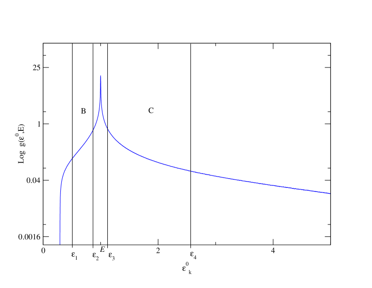
Figure 2: Eigenfunction tail zones B and C considered for analysis. The extreme cutoffs are determined by the quantum classical agreement, and renormalized for unfolding. The center window is $4\Delta$ and $80\Delta$ width for the corresponding cases analyzed here.

Figure 3: Amplitude distribution for the unfolded EF with energies $E_{100}=204.013$ (a)-(b) and $E_{900}=846.680$ (c)-(d) in zones B and C. The Gaussian with the same moments as the distributions are indicated by the continuous line. Note that (b) is plotted in semilogarithmic scale.

Figure 4: Averaged eigenfunction around $\psi_{500}$ for $H_{2}$ Hamiltonian in the $H_{1}$ basis with the parameters given in the text and at energy $E_{500}=611.717$. The smooth curve represents the corresponding classical EF.

Figure 5: Amplitude distribution for the unfolded EF $E_{500}=611.717$ of $H_{2}$ Hamiltonian in the zone B (a) and C (d). The Gaussian with the same moments as the distributions are showed by the continuous line.

Figure 6: Histogram of the amplitudes distribution in a window of width of 20 energy units for 100 EFs around (a)$\psi_{900}$ of $H_{1}$ and (b)$\psi_{500}$ of $H_{2}$. The normalization corresponds to the number of events per bin, the total number of events being 2525 and 2595 for (a) and (b), respectively. The corresponding values of $\chi^{2}$ are $\chi_{16}^{2}=12.289$ and $\chi_{16}^{2}=14.483$. The continuous line corresponds to a Gaussian curve with the same moments as the histograms.

References

- [1] Berry M V and Tabor M 1977 Proc. R. Soc. London A 356 375; Casati G, Guarneri I and Valz-Gris F 1980 Lett. Nuovo Cimento 28 279; Bohigas O, Giannoni M-J and Schmit C 1983 Phys. Rev. Lett. 52 1; Berry M V 1985 Proc. R. Soc. London A 400 229; Leyvraz F and Seligman T H 1992 Phys. Lett. A 168 348.
- [2] Mehta M L 1990 Random Matrix Theory and Statistical Theory of Energy Levels ( New York: Academic Press); Brody T A, Flores J, French J B, Mello P A, Pandey A and Wong S S M 1981 Rev. Mod. Phys. 53 385; Guhr T, Müller-Groeling A and Weidenmüller H A 1998 Phys. Rep. 299 189.
- [3] Flambaum V V, Gribakina A A, Gribakin G F and Kozlov M G 1994 Phys. Rev. A 50 267 ().
- [4] Luna-Acosta G A, Méndez-Bermúdez J A and Izrailev F M 2001 Phys. Rev. E 64 036206.
- [5] Benet L, Izrailev F M, Seligman T H and Suarez-Moreno A 2000 Phys. Lett. A 277 87.
- [6] Heller E J 1984 Phys. Rev. Lett. 53 1515.
- [7] Kaplan L1999 Nonlinearity 12 R1. See references therein. See also Sridhar S, Lu W T 2002 J. Stat Phys. 108 755. Wisniacki D A, Borondo F, Vergini E and Benito R M (2001) it Phys. Rev. E 65 016213.
- [8] Benvenuto F, Casati G, Shepeliansky D L 1997 Phys. Rev A 55 1732.
- [9] Berry M V 1977 J. Phys. A: Math. Gen 10 2083.
- [10] Benet L, Flores J, Hernández-Saldaña H, Izrailev F M, Leyvraz F and Seligman T H to appear.