Frequency Dependence of Quantum Localization
in a Periodically Driven System

Abstract

We study the quantum localization phenomena for a random matrix model belonging to the Gaussian orthogonal ensemble (GOE). An oscillating external field is applied on the system. After the transient time evolution, energy is saturated to various values depending on the frequencies. We investigate the frequency dependence of the saturated energy. This dependence cannot be explained by a naive picture of successive independent Landau-Zener transitions at avoided level crossing points. The effect of quantum interference is essential. We define the number of Floquet states which have large overlap with the initial state, and calculate its frequency dependence. The number of Floquet states shows approximately linear dependence on the frequency, when the frequency is small. Comparing the localization length in Floquet states and that in energy states from the viewpoint of the Anderson localization, we conclude that the Landau-Zener picture works for the local transition processes between levels.

1 Introduction

The diffusive phenomena have been actively studied in quantum systems with a complex level structure in the presence of a periodic external field. Under a periodic perturbation, when a system shows so-called quantum chaotic nature, it is widely believed that energy diffusion of the system eventually ceases and the energy saturates at a finite value. So far, only limited number of these systems have been actually studied. The kicked rotator model [1] and the kicked top model [2] are typical quantum models which show the quantum chaotic nature under a periodic external field. The difference between classical and quantum energy diffusion has been discussed by investigating these models. In the quantum kicked rotator model, starting initially from the ground state, the system evolves diffusively only for a finite time. After then the diffusive time-evolution ceases and the average energy is saturated to a finite value. That is, the system cannot absorb energy after that time. This is a remarkable difference from the classical diffusion, where the energy increases unlimitedly. The mechanism of this quantum localization in the model was discussed in the context of the Anderson localization [3, 4]. Recently the kicked rotator model is experimentally realized using Hydrogen and Sodium atoms, and the quantum localization is observed [5, 6, 7, 8, 9].

It is known that random matrices well describe characteristics of the level statistics of the systems which show chaotic nature in the corresponding classical models[10, 11]. Therefore we study the quantum localization process of random matrices to extract universal features. In this paper, we investigate the time evolution of a system whose Hamiltonian is taken from the Gaussian orthogonal ensemble (GOE) with a periodic perturbation, and try to capture the universal features on the relation between the saturated energy and the frequency of the perturbation. So far, several types of time-dependent random matrices are adopted to study the quantum diffusion process [12, 14, 15, 13]. Wilkinson calculated the energy diffusion constant using the Landau-Zener transition formula[16, 17, 18] when the perturbation acts on the system linearly in time.[13] He clarified the difference of diffusion constants between GOE and the Gaussian unitary ensemble (GUE). Wilkinson neglected the effect of interference of quantum phase, which plays a crucial role in the quantum localization in the presence of periodic perturbation [14]. Cohen and Kottos considered the energy diffusion before the saturation in the Wigner’s banded random matrix (WBRM) model with an oscillating perturbation, and calculated the diffusion coefficient as a function of the amplitude and frequency of the perturbation [12]. Taking these previous studies into account, we study how the Landau-Zener picture is related to the quantum localization by investigating the dependence of the saturated energy on the frequency of the perturbation.

We first numerically demonstrate that the quantum localization occurs in the system, which cannot be explained by a naive application of an independent Landau-Zener picture to the system. In order to understand the quantum localization intuitively, we consider the overlap between Floquet eigenstates and the initial ground state, and find that the overlap exponentially decays in the Hilbert space spanned by Flouqet eigenstates, which directly means that the ground state is localized in this representation. We define the relevant number of Floquet eigenstates which has a large overlap with the initial ground state. This number was originally introduced as a quantity which corresponds to the Lyapunov exponent in the quantum kicked top model by Haake et al.[2]. The dependence of the relevant number on the frequency is numerically investigated. We numerically find that this number linearly depends on the frequency of the perturbation in small frequency regime. Employing a plausible proportional relation between the localization length in the energy space and that in the Floquet space, which is also adopted in the case of the kicked rotator model, and taking account of this linear dependence, we find the Landau-Zener mechanism works in the view of the Anderson localization.

This paper is organized in the following way. In §2, we explain the random matrix model and the numerical method of time evolution. In §3, we study the frequency dependence of the saturated average energy. In §4, we discuss the quantum localization by introducing the number of relevant Floquet states. Finally in §5, we give summary and discussion.

2 Model and Method

We consider time-reversal invariant systems under an oscillating external field. The random matrix ensemble appropriate for describing the spectral statistics of these systems is the Gaussian orthogonal ensemble (GOE). Random matrices well describe characteristics of energy spectra of complex quantum systems which have no conserved quantities.

We shall consider the total Hamiltonian given by

$$\mathcal{H}(t)=H_{0}+\lambda(t)V,$$ (1)

where $H_{0}$ denotes the non-perturbed part of the Hamiltonian, and $\lambda(t)V$ is the perturbation part with a time-dependent parameter $\lambda(t)$. We take $H_{0}$ and $V$ from the ensemble of the GOE random matrices with the dimension $N$. This model corresponds to the realistic systems such as billiard systems with a time-dependent boundary, or complex spin systems with a time-dependent external field. Matrix elements ${H_{0}}_{ij}$ and $V_{ij}$ are taken from independent Gaussian random variables with mean zero and with the variance: ${\rm var}\left({H_{0}}_{ij}\right)=1+\delta_{ij}$ and ${\rm var}\left(V_{ij}\right)=1+\delta_{ij}$. Note that both of the non-perturbed and perturbed terms have the same statistical properties. The density of states $\rho(E)$ at the energy $E$ is given by Wigner’s semicircle law for large $N$ [19],

$$\rho(E)=\frac{1}{2\pi N}\sqrt{4N-E^{2}}.$$ (2)

In this paper, we confine $\lambda(t)$ to the sinusoidal form, $\lambda(t)=A\sin(\omega t)$ with $A=0.5$. Eigenvalues of a GOE random matrix show a structure with level repulsion as a function of $\lambda$. Energy spectrum of a system of $N=500$ around the ground state, and around the center ($E=0$) are depicted in Fig. 1 (a) and (b), respectively. Many avoided crossings are seen in Figs. 1. There are no degeneracies of levels although some energy levels are seen to be crossing due to the line width.

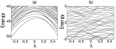
Figure 1: Energy spectrum of $\mathcal{H}$ for $N=500$ as a function of $\lambda$ around (a) the ground state and (b) the center.

Now we consider the time evolution of a state $|\psi\rangle$ of the system;

$${\rm i}\frac{\partial}{\partial t}|\psi\rangle=\mathcal{H}(t)|\psi\rangle.$$ (3)

Here we take $\hbar=1$ and the initial state $|\psi_{0}\rangle$ is taken to be the ground state. The state $|\psi_{1}\rangle$ after a period $T=2\pi/\omega$ from $t=0$ is expressed using the Floquet operator[20] $F$;

$$|\psi_{1}\rangle=F|\psi_{0}\rangle,\quad F\equiv{\rm T}\exp\left[-{\rm i}\int_{0}^{2\pi/\omega}\mathcal{H}(t){\rm d}t\right],$$ (4)

where ${\rm T}$ means the time ordered product. Therefore the state after the $n$th period $|\psi_{n}\rangle$ is written as

$$|\psi_{n}\rangle=F^{n}|\psi_{0}\rangle.$$ (5)

Floquet eigenvectors $\left\{|\nu\rangle\right\}$ form a complete set in the Hilbert space, and Floquet eigenvalues are aligned on a unit circle of the complex plane;

$$F|\nu\rangle=e^{{\rm i}\phi_{\nu}}|\nu\rangle.$$ (6)

We calculate $F$ numerically by integrating the Schrödinger equation (3) for a period using the fourth order decomposition of time-evolution operator [21]. The time evolution of energy is expressed in terms of Floquet eigenvalues and eigenstates. The energy after the $n$th period is expressed using the Floquet operator;

$$\langle\psi_{n}|\mathcal{H}|\psi_{n}\rangle =\langle\psi_{0}|(F^{\dagger})^{n}\mathcal{H}F^{n}|\psi_{0}\rangle$$

$$=\sum_{\nu^{\prime},\nu}e^{{\rm i}n(\phi_{\nu}-\phi_{\nu^{\prime}})}\langle\psi_{0}|\nu^{\prime}\rangle{}\langle\nu|\psi_{0}\rangle{}\langle\nu^{\prime}|\mathcal{H}|\nu\rangle.$$ (7)

3 $E_{\rm sat}$ as a Function of $\omega$

3.1 Numerical results

We define $g(\nu,\nu^{\prime})$ and $E_{\rm sat}$ as,

$$g(\nu,\nu^{\prime}) \equiv\langle\psi_{0}|\nu\rangle\langle\nu|H_{0}|\nu^{\prime}\rangle\langle\nu^{\prime}|\psi_{0}\rangle,$$

$$E_{\rm sat} \equiv\sum_{\nu}g(\nu,\nu),$$ (8)

and rewrite eq. (7) as,

$$\langle\psi_{n}|H_{0}|\psi_{n}\rangle =\sum_{\nu^{\prime},\nu}e^{{\rm i}n(\phi_{\nu^{\prime}}-\phi_{\nu})}g(\nu,\nu^{\prime})$$

$$=E_{\rm sat}+\sum_{\nu<\nu^{\prime}}\left(e^{{\rm i}n(\phi_{\nu^{\prime}}-\phi_{\nu})}g(\nu,\nu^{\prime})+\mbox{c.c.}\right).$$ (9)

In the second term of the right-hand side of eq. (9), the expectation values of terms for $\{\nu\neq\nu^{\prime}\}$ oscillates with the period $2\pi/(\phi_{\nu^{\prime}}-\phi_{\nu})$. Thus, we see $\langle\psi_{n}|H_{0}|\psi_{n}\rangle$ fluctuates around $E_{\rm sat}$. Therefore, $E_{\rm sat}$ is regarded as the saturated value of the energy.

Figure 2 shows the time evolution of $\langle\psi_{n}|H_{0}|\psi_{n}\rangle$ (zigzag curve), and the corresponding $E_{\rm sat}$ (horizontal line) with respect to $\omega/\pi=$ 0.02, 0.1, 0.2, 0.4, and 1.0 for $N=500$. Figure 3 shows $E_{\rm sat}$ as a function of $\omega$ obtained from five samples for $N=256$, $500$, and $700$. We should note that the maximal saturated energy is zero because the energy spectrum is symmetric about zero energy (E=0), and this maximal energy corresponds to the high temperature limit. Here we normalize $E_{\rm sat}$ such that the distance between $E=0$ and the ground state is $1$. Indeed in classical systems, the energy diffusion continues forever, which means that $E_{\rm sat}$ converges to $0$.

On the other hand, when $\omega$ is very small ($\omega=0.02\pi$), the time evolution of the system is almost adiabatic, and the average energy changes little.[22] When $\omega$ becomes slightly larger ($\omega=0.1\pi\mbox{ and }0.2\pi$), transitions between levels begin to occur at avoided crossings (that is, nonadiabatic transitions). Thus the system absorbs energy and $E(t)$ increases. However $E(t)$ saturates before it reaches to 0. The value of $E_{\rm sat}$ gradually approaches to the center of the energy spectrum ($E_{\rm sat}=0$) as $\omega$ grows larger ($\omega=0.4\pi\mbox{ and }1.0\pi$). These finite saturations of $E_{\rm sat}$ are caused by the quantum effects, and this feature is called the quantum localization [1, 10]. The quantum localization was first discovered in the kicked rotator model, which shows chaotic motion in the classical limit.[1]

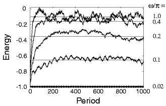
Figure 2: Zigzag curves represent the time evolution of the average energy $E(t)$. Horizontal lines represent $E_{\rm sat}$. A pair of $E(t)$ and $E_{\rm sat}$ denotes, from the bottom, data for $\omega=$ $0.02\pi$, $0.1\pi$, $0.2\pi$, $0.4\pi$, and $1.0\pi$.

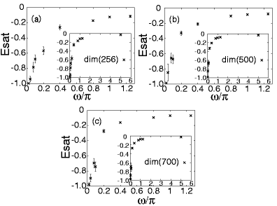
Figure 3: $E_{\rm sat}$ as a function of $\omega$ for (a) $N=256$, (b) $N=500$, and (c) $N=700$. Errorbars show the variance among the data obtained from five samples.

3.2 Failure of a Picture of Independent Landau-Zener Transitions

As shown in the previous section, the energy is saturated to a finite value. We here show that this saturation cannot be realized without considering the quantum interference effect. Let us consider the small frequency regime where transitions between energy levels take place only between the two levels at an avoided level crossing point. In such a region, we can introduce the well-known Landau-Zener picture for each transition. Wilkinson proposed a theory of the evolution of the energy in a random matrix model with a time-dependent perturbation.[13] His theory assumes that transitions take place only at avoided crossings and the transition probability is determined by the Landau-Zener formula[17]. This implies that the sweeping speed of the parameter is sufficiently slow, and there multiple level scatterings are not relevant. In the case that the field increases linearly in time, he found that this approximation of independent Landau-Zener scattering gives a good result.[14]

If we apply a simple independent Landau-Zener picture to our case , we will find,

$$E_{\rm sat}=0.$$ (10)

In what follows, we derive eq. (10). We assume that each transition occurs at an avoided level crossing point and the probability is given by the Landau-Zener formula. Let us consider the transition rate $R$ which is the probability per unit time that the system makes a transition to one of the two neighboring states. This quantity $R$ was already given for the case where the external field increases linearly in time [13]. We apply the known expression to the present oscillating case. The transition rate $R$ is determined by statistical distributions of the energy gaps and the asymptotic slopes at avoided crossing points. The average speed of the parameter $\lambda(t)$ is denoted by $\bar{|\dot{\lambda}|}$. For the present oscillating field, $\bar{|\dot{\lambda}|}$ is roughly estimated as $\bar{|\dot{\lambda}|}\simeq A\omega$. In addition, let $\rho$ denote the density of states and $\bar{\sigma}$ denote the typical difference between the asymptotic slopes of an avoided crossing. Under the conditions of slow speed, $\hbar\bar{\sigma}|\bar{\dot{\lambda}}|\rho^{2}\ll 1$, which corresponds to the situation that transitions of states only occur at avoided crossings to the adjacent levels, $R$ is expressed as,

$$R\propto\hbar^{1/2}\bar{\sigma}^{1/2}|\bar{\dot{\lambda}}|^{3/2}\rho^{2}\propto\hbar^{1/2}|\bar{\dot{\lambda}}|^{3/2}\rho^{3/2}.$$ (11)

We consider the time evolution of the occupation probability for the eigenstate with energy $E$ at time $t$, $f(E,t)$. We can derive the diffusion equation for the occupation probability $f(E,t)$ of the state by extending Wilkinson’s theory to the case that $\rho(E)$ is not constant;

$$\frac{\partial\rho f}{\partial t}+|\bar{\dot{\lambda}}|\frac{\partial}{\partial E}\left(\frac{dE}{d\lambda}\rho f\right)=\frac{\partial}{\partial E}\left[D\rho\frac{\partial f}{\partial E}\right],$$ (12)

where $D=R/{\rho^{2}}$. Using the equation of continuity:

$$\frac{\partial\rho}{\partial t}+|\bar{\dot{\lambda}}|\frac{\partial}{\partial E}\left(\frac{dE}{d\lambda}\rho\right)=0,$$ (13)

eq. (12) is rewritten as,

$$\rho\frac{\partial f}{\partial t}=-|\bar{\dot{\lambda}}|\frac{dE}{d\lambda}\rho\frac{\partial f}{\partial E}+\frac{\partial}{\partial E}\left[D\rho\frac{\partial f}{\partial E}\right].$$ (14)

Let us consider the steady state $f(E)=f(E,\infty)$. Then the left-hand side of eq. (14) gives zero. Note that $\rho$ is given by the semicircle law (2), $\rho(E)=\frac{1}{2\pi N}\sqrt{L^{2}-E^{2}}\,(L=2\sqrt{N})$ when $N$ is very large. Therefore, $f(E)$ is solved as

$$f(E)=\int_{-L}^{E}c_{1}\exp\left[\int_{-L}^{E^{\prime}}k(\epsilon){\rm d}\epsilon\right]{\rm d}E^{\prime}+c_{0},$$ (15)

where $c_{0}$ and $c_{1}$ are constants of integration, and

$$k(E)\equiv\frac{1}{D}\left(|\bar{\dot{\lambda}}|\frac{dE}{d\lambda}-\rho^{-1}\frac{\partial(D\rho)}{\partial E}\right).$$ (16)

When we integrate eq. (15), the second term of $k(\epsilon)$ diverges, because

$$\int_{-L}^{E^{\prime}}-\frac{1}{D\rho}\frac{\partial D\rho}{\partial\epsilon}{\rm d}\epsilon\propto-\int_{-L}^{E^{\prime}}\frac{{\rm d}\ln\rho}{{\rm d}\epsilon}{\rm d}\epsilon\rightarrow-\infty,$$ (17)

where we used $D=R/\rho^{2}$ and eq. (11). Therefore,

$$f(E)=c_{0}.$$ (18)

As a result, the average energy always becomes $0$ (the center of the energy spectrum);

$$E_{\rm sat}=\int E\rho f(E){\rm d}E=0.$$ (19)

Thus we find that the idea of independent Landau-Zener scattering is not applicable at least to a periodic system.[14, 23]. We cannot ignore the quantum mechanical interference effect for the quantum localization.

3.3 Phenomenological Interpretation of the Quantum Localization in Analogy to the Anderson Localization

We here phenomenologically interpret the quantum localization. The quantum localization in the present system reminds us the Anderson localization where a particle in the presence of a random potential is spatially localized [24]. The system for the Anderson localization is described by the Hamiltonian:

$$\mathcal{H}_{\rm A}=\sum_{i}v_{i}|i\rangle\langle i|+t\sum_{\langle i,i^{\prime}\rangle}|i\rangle\langle i^{\prime}|.$$ (20)

Here, $|i\rangle$ means the state of the particle at the $i$th site, $v_{i}$ is the value of a random potential at the site $i$ which is uniformly distributed with a width $W$, and $t$ represents hopping to one of the nearest neighbor sites. In this particle system, the average hopping probability $p_{\rm A}$ is expressed as $p_{\rm A}\sim|t|/W$. The probability $p_{\rm A}(m)$ that the particle exists on the $m$th site from the initial ($0$th) site is estimated as $p_{\rm A}(m)\sim p_{\rm A}^{m}\sim\exp\left(-m\log(W/|t|)\right)$.[25] That is, the particle is localized in the space exponentially. This localization is caused by the quantum interference effects.

Let us consider the analogy to the Anderson localization in the quantum localization of the present model. We associate the state $|i\rangle$ in eq. (20) with the $i$th adiabatic state of $H_{0}$. Furthermore we focus on the frequency regime where transitions between levels take place only at avoided crossings. We numerically confirmed that this situation is actually realized for small $\omega$. In this case, we define a transition probability $p_{\rm Q}$ between adjacent levels, which corresponds to $p_{\rm A}$ in the Anderson localization, and we find the common characteristics between the present situation in the random matrices and the Anderson localization. That is, the localization occurs due to the quantum inference effect among many transitions between states. We may write the occupation probability $p_{\rm Q}(m)$ that a state is on the $m$th level as $p_{\rm Q}(m)\sim p_{\rm Q}^{m}$, where $p_{\rm Q}$ is a transition probability between the states. Actually fast relaxation is observed numerically in $p_{\rm Q}(m)$ of a typical example, which is depicted in Fig. 4.

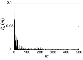
Figure 4: The probability $P_{\rm Q}(m)$ that the state is on the $m$th level of the system (1) for $N=500$ and $\omega=0.1\pi$. It is obtained after 600 periods.

If we assume an exponential form in the analogy to the Anderson localization, the saturation energy $E_{\rm sat}$ is written as,

$$E_{\rm sat}=\sum_{m=1}^{N}p_{\rm Q}^{(m-1)}E_{m}/Z,$$ (21)

where $E_{m}$ is the $m$th eigenvalue of $H_{0}$ and $Z$ is the normalization factor, $Z=\sum_{m=1}^{N}p_{\rm Q}^{m-1}$. Equation (21) gives a finite saturation value of $E_{\rm sat}$.

4 The Relevant Number of Floquet Eigenstates

In previous sections, we showed the quantum localization in the random matrix model and considered an intuitive interpretation. In this section, we consider the quantum localization from the viewpoint of the Floquet theory. As seen in eq. (8), the quantum dynamics is determined by the overlaps between the initial state and Floquet eigenstates, i.e., $|\langle\nu|\psi_{0}\rangle|^{2}$, and $E_{\rm sat}$ is obtained by Floquet eigenstates. Thus we here discuss this overlap.

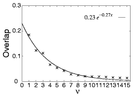
Figure 5: The dependence of the overlap $|\langle\nu|\psi_{0}\rangle|^{2}$ on the number $\nu$. $|\langle\nu|\psi_{0}\rangle|^{2}$ is arranged in order of the magnitude. The overlap decays exponentially. Here $\omega=0.1\pi$ and $N=500$.

We found numerically that the distribution of $|\langle\nu|\psi_{0}\rangle|^{2}$ decays approximately following an exponential function when we arrange the states in order of the magnitude of the overlap as is shown in Fig. 5. This property is one of the characteristics of the quantum localization. We study how many Floquet states are involved in the ground state, and define the minimal number $N_{\rm min}$ of the Floquet states by which the initial state $|\psi_{0}\rangle$ is covered within a ratio $r$:

$$N_{\rm min}=\frac{1}{N}\min\left\{\mathcal{N}_{\rm min}:\sum_{\nu=1}^{\mathcal{N}_{\rm min}}|\langle\psi_{0}|\nu\rangle|^{2}>r;|\langle\psi_{0}|\nu\rangle|^{2}\geq|\langle\psi_{0}|\nu+1\rangle|^{2}\right\}.$$ (22)

This quantity is the same as the quantity used in the different context by Haake, Kus, and Scharf.[2] Here, we take $r=0.99$. Figure 6 shows $N_{\rm min}$ as a function of $\omega/\pi$ obtained from five samples for $N=256$, $500$, and $700$.

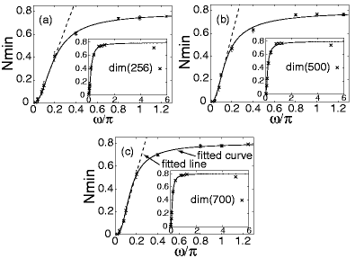
Figure 6: $N_{\rm min}$ as a function of $\omega/\pi$ for (a) $N=256$, (b) $N=500$, and (c) $N=700$. Errorbars show the variance among the data obtained from five samples. The fitted line and also linear fitting in the intermediate region are shown in each graph.

We introduce the fitting function for $N_{\rm min}(\omega)$ in the form:

$$N_{\rm min}(\omega)=N^{*}_{\rm min}\left\{1-\frac{1}{\left[(\omega/\omega^{*})^{a}+1\right]^{b}}\right\}.$$ (23)

This function fits the data quite well. In eq. (23), $N^{*}_{\rm min}$, $a$, $b$, and $\omega^{*}$ are determined from the least-squares method. The results are shown in Table 4. From eq. (23), $N_{\rm min}(\omega)$ is extremely small when $\omega\ll\omega^{*}$. This is partially because the energy gaps in lower energy region are so large comparing with $\omega$ that transition to higher levels from the ground state seldom occurs (see Fig. 1(a)), and therefore the system behaves almost adiabatically.[22] On the other hand, $N_{\rm min}(\omega)$ is well fitted by a linear function (dashed line) for the region of $\omega\sim\omega^{*}$.

Table 1: Values of the parameters in eq. (23) obtained by the least-squares method.

@  cccc variablesdim(256)dim(500)dim(700)
$N^{*}_{\rm min}$ 0.79 0.80 0.80
a 2.3 2.6 3.0
b 0.67 0.47 0.54
$\omega^{*}/\pi$ 0.15 0.10 0.11

So far, we observed localization in the energy space and also in the space of Floquet states. Now we discuss on localization length of the two localizations. In particular, we focus on the linear dependence of $N_{\rm min}(\omega)$ on $\omega$ in the small $\omega$ region. We employ a phenomenological argument using the analogy to the Anderson localization as explained in §3.3. Let us express the transition probability $p_{\rm Q}$ using some function $\Gamma(\omega)$ in the form:

$$p_{\rm Q}\sim\exp\left[-\Gamma^{-1}(\omega)\right].$$ (24)

The occupation probability $p_{\rm Q}(m)$ that a stationary state is on the $m$th level is expressed as $p_{\rm Q}(m)\sim p_{\rm Q}^{m}\sim\exp\left[-\Gamma^{-1}(\omega)m\right]$. Thus we can regard $\Gamma(\omega)$ as the localization length in the energy space. Now let $l$ denote the localization length in the Floquet space, i.e., $|\langle\nu|\psi_{0}\rangle|^{2}\simeq ce^{-\nu/l}$, where $c$ is the normalization constant. From the definition (22), $N_{\rm min}$ is expressed using the length $l$ as

$$N_{\rm min}\simeq-\frac{l}{N}\ln(1-r)\propto l.$$ (25)

Since we now focus on the linear dependence of $N_{\rm min}$ on $\omega$, we write,

$$N_{\rm min}=\alpha\omega+\beta,$$ (26)

where $\alpha$ and $\beta$ are constants. We note that $\beta$ is negligibly small. Then we have

$$l\propto\omega.$$ (27)

As has been assumed in the the kicked rotator model to discuss the diffusion constant [26], we assume the proportionality between $l$ and $\Gamma(\omega)$,

$$l\propto\Gamma(\omega).$$ (28)

Then, we obtain from eqs. (27) and (28),

$$\Gamma(\omega)=\omega/h.$$ (29)

Here $h$ is an unknown amplitude which may depend on $N$, $A$, the typical size $\bar{\epsilon}$ of gaps at avoided crossings, and the difference $\bar{\sigma}$ of the two asymptotic slopes at an avoided crossing. This $\omega$ dependence is consistent with that of the Landau-Zener formula, because eqs. (24) and (29) give

$$p_{\rm Q}\sim\exp\left[-\frac{h}{\omega}\right].$$ (30)

Actually, we numerically confirmed that transitions between levels take place only at avoided crossings in the region where $N_{\rm min}$ linearly depends on $\omega$. Thus we suppose that the amplitude of local transition probability is originated in the Landau-Zener transition, although the phase interference has an important effect on the global phenomena.

5 Summary and Discussion

We have studied numerically the time evolution of the average energy of the GOE random matrix model under a perturbation of a sinusoidal function of time. In §3, we showed that the quantum localization occurs in this model. We have also studied the frequency dependence of the saturated energy $E_{\rm sat}$, and we showed that we can not rely on the picture of independent occurrence of Landau-Zener transitions in the present case because the suppression of the quantum diffusion is essentially due to the phase interference effect of quantum mechanics. We discuss this quantum localization in analogy to the Anderson localization. In §4, we introduced the relevant number of Floquet states $N_{\rm min}$, and proposed a form of $N_{\rm min}$ as a function of $\omega$. $N_{\rm min}$ is almost zero when $\omega$ is nearly zero, and it saturates when $\omega$ is sufficiently large. In the intermediate region, $N_{\rm min}$ grows linearly as $\omega$ increases. This linear dependence of $N_{\rm min}$ on $\omega$ implies that the localization length $l$ in the Floquet eigenstates also depends linearly on $\omega$ (eq. (25)). On condition that $\Gamma\propto l$, the localization length $\Gamma$ of the eigenstates of the Hamiltonian is also proportional to $\omega$. This dependence of $\Gamma$ on $\omega$ implies the Landau-Zener mechanism governs the local transitions.

Acknowledgments

This study is partially supported by Grant-in-Aid from the Ministry of Education, Culture, Sports, Science and Technology of Japan. The computer calculation was partially carried out at the computer center of the ISSP, which is gratefully acknowledged.

References

- [1] G. Casati, B.V. Chirikov, J. Ford, and F.M. Izrailev: Lecture Notes Phys.93(1979)334.
- [2] F. Haake, M. Kus, and R. Scharf: Z.Phys.B65(1987)381.
- [3] S. Fishman, D.R. Grempel, and R.E. Prange: Phys.Rev.Lett.49(1982)509.
- [4] D.R. Grempel, R.E. Prange, and S. Fishman: Phys.Rev.A29(1984)1639.
- [5] E.J. Galvez, B.E. Sauer, L. Moorman, P.M. Koch, and D. Richards: Phys.Rev.Lett.61(1988)2011.
- [6] J.E. Bayfield, G. Casati, I. Guarneri, and D.W. Sokol: Phys.Rev.Lett.63(1989)364.
- [7] M. Arndt, A. Buchleitner, R.N. Mantegna, and H. Walther: Phys.Rev.Lett.67(1991)2435.
- [8] F.L. Moore, J.C. Robinson, C. Bharucha, P.E. Williams, and M.G. Raizen: Phys.Rev.Lett.73(1994)2974.
- [9] G.P. Collins: Phys.Today48(1995)18.
- [10] F. Haake: Quantum Signatures of Chaos(Springer,Berlin,2001)2nd ed.
- [11] H.-J. Stöckmann: Quantum Chaos(Cambridge Univ. Press,Cambridge,1999).
- [12] D. Cohen and T. Kottos: Phys.Rev.Lett.85(2000)4839.
- [13] M. Wilkinson: J.Phys.A21(1988)4021.
- [14] M. Wilkinson: Phys.Rev.A41(1990)4645.
- [15] A. Bulgac, G.D. Dang, and D. Kusnezov: Phys.Rev.E54(1996)3468.
- [16] L. Landau: Phys.Z.Sowjun.2(1932)46.
- [17] C. Zener: Proc.R.Soc.LondonA137(1932)696.
- [18] E.G.C. Stueckelberg: Helv.Phys.Acta.5(1932)369.
- [19] E.P. Wigner: Proc.4th.Can.Math.Congr.,Toronto,1959(1959) p.174.
- [20] G. Floquet: Ann. de l’Ecole Norm.Sup.XII(1883)47.
- [21] M. Suzuki: Phys.Lett.A146(1990)319.
- [22] A. Joye, H. Kunz, and Ch.-Ed. Pfister: Ann.Phys.208(1991)299.
- [23] Y. Gefen and D.J. Thouless: Phys.Rev.Lett.59(1987)1752.
- [24] P.W. Anderson: Phys.Rev.109(1958)1492.
- [25] Y. Nagaoka: Prog.Theor.Phys.84(1985)Suppl,p.1.
- [26] T. Dittrich and R. Graham: Ann.Phys.200(1990)363.