Classical Mechanics of a Three Spin Cluster

Abstract

A cluster of three spins with single-axis anisotropic exchange coupling exhibits a range of classical behaviors, ranging from regular motion at low and high energies to chaotic motion at intermediate energies. A change of variable makes it possible to isolate total angular momentum around the z-axis (a conserved quantity) and it’s associated cyclic variable from two non-trivial degrees of freedom. This clarifies the interpretation of Poincaré sections, and causes permutation symmetries of the system to manifest as rotation symmetries in the new coordinates.

The three-spin system has four families of periodic orbits (multiple instances of each orbit exist because of permutation symmetry.) Analysis of spin waves predicts their periods in the low energy (antiferromagnetic) and high energy (ferromagnetic) limits and also can be used to determine the stability properties of certain orbits at intermediate $E=-1.$ The system also undergoes interesting changes in the topology of the energy surface along particular curves in energy-parameter space, for instance, when two pieces of the energy surface surrounding the two antiferromagnetic fixed points coalesce. Poincarésections produced with a 3-d graphic technique (described in the Appendix) illustrate the symmetries of the system and illustrate the transition to chaos at low energies.

The three spin system turns out to have similarities with the Anisotropic Kepler Problem (AKP) and the Hénon-Heiles Hamiltonian. An appendix discusses numerical integration techniques for spin systems. The quantum manifestations of the structures found in this paper are discussed in [P. A. Houle, N. G. Zhang, C. L. Henley, Phys. Rev. B 60 15179 (1999)].

I Introduction

This paper is a study of the classical mechanics of a cluster of three spins with single-axis anisotropic exchange coupling; the Hamiltonian of the system is

$$H=J\left[\sum_{1\leq i<j\leq 3}\;{{\bf S}}_{i}\cdot{{\bf S}}_{i+1}-\sigma S_{iz}S_{(i+1)z}\right],$$ (1)

We can set $J=1$ without losing generality (even the sign is arbitrary for our study of the dynamics). @@ Eq. (1) is a model for spin clusters in triangular antiferromagnets such as $\mathrm{NaTiO_{2}}$ and $\mathrm{RbFeCl_{3}}.$ It was introduced in Nakamura et al. (1985) and is further reported on in Nakamura et al. (1986); Nakamura and Bishop (1986); Nakamura (1993). In these works, Nakamura studied the level statistics of the system, and compared the behavior of energy level fluctuations as a function of $\sigma$ in regions where the classical dynamics was predominantly regular and chaotic. In a previous work, we’ve discussed how the classical structures of the system are manifested in its quantum spectrum Houle et al. (1999).

This system is of intrinsic interest as a comparatively simple dynamical system possessing high symmetry. We were specifically motivated by semiclassics, i.e. the relation between classical dynamics and the eigenstates of a quantum system.

The quantum manifestations of classical chaos were investigated not only on the model of Eq. (1), but also in a cluster of two interacting spins Magyari et al. (1987); Srivastava et al. (1988, 1990); Srivastava and Müller (1990a, b); Srivastava et al. (1991). The method of Bohr-Sommerfeld quantization has also been applied, but to single spins Shankar (1980); Klein and Li (1981).

In recent years, a variety of magnetic molecules have been synthesized containing clusters of interacting spins Sessoli (1981). Although commonly approximated as a single moment, they do have internal excitations which cannot be found exactly by exact diagonalization (since the Hilbert space is too large). If the spin cluster divides into subclusters, each of which has a moderately long moment, these excitations may best be grasped semiclassically. The methods of the present paper would be a natural starting point for such studies, at least for systems with high symmetry.

Eq. (1) conserves total $S_{z}=\sum_{i=1}^{3}S_{iz}.$ A key aspect of our approach is a change of variable which separates the system into two subsystems: (i) A nonintegrable two-degree of freedom subsystem, and (ii) a single degree of freedom subsystem for which total $S_{z}$ is a conserved momentum variable. Our change of variable makes the Poincaré sections comprehensible [in contrast to prior work Nakamura (1993) that did not separate subsystems (i) and (ii)], and makes it easy to find the fundamental periodic orbits of the system. As in previous work on Eq. (1), we restrict our consideration to the special case that $S_{z}=0;$ as this paper considers only the classical mechanics of the system, we set $|{\bf S}|=1$ without losing generality.

An outline of this paper follows: Section II introduces our change of variable and shows how the topology of the phase space and the symmetries of the system appear in the new coordinates. Section III is a discussion of the fixed points, invariant manifolds, and spin waves of the three-spin system. Section IV is about changes in the topology of the energy surface that occur along certain curves in the $E-\sigma$ parameter space. Section V enumerates the fundamental periodic orbits of the system and maps the global dynamics of the system with Poincaré sections. Section VI concludes by discussing similarities between the the three-spin cluster and the well-studied Anisotropic Kepler Problem and the Hénon-Heiles Hamiltonian.

II Hexagonal phase space

With three degrees of freedom, the dynamics of an arbitrary dynamical system is difficult to visualize and understand. Fortunately, the three-spin cluster conserves total angular momentum around the z-axis, so we can separate the problem into two halves: (i) an autonomous nonintegrable two degree of freedom Hamiltonian, and (ii) an trivial single degree of freedom system which is driven by system (i). Part (i) can be studied in isolation from part (ii), however, since (ii) is driven by (i) we must solve the motion of (i) before we can solve the motion of (ii).

Section II.1 presents a change of variable that separates part (i) from part (ii) – which is necessary to draw useful Poincaré sections. Next, Section II.2 shows how the discrete symmetries of the system appear in the new coordinates. Then, in Section II.3 we’ll show that the $2\pi$ periodicity of the spin longitudes $(\phi_{i})$ manifests as hexagonal tiling in the $(\Phi_{A},\Phi_{B})$ coordinates.

II.1 A change of coordinates

The conventional canonical coordinates for spin are $(\phi_{i},z_{i})$ where $\phi_{i}$ is longitude and $z_{i}=S_{iz}.$ Van Hemmen and Sütö (1986) Spin space includes both position and momentum and is the complete phase space of a spin system – the position of the spin vectors at a moment in time completely describes the system. The mapping between $(\phi_{i},z_{i})$ and spin vector components is ${{\bf S}_{i}}=\{S_{ix},S_{iy},S_{iz}\}=\{(1-z_{i}^{2})^{1\over 2}\cos\phi_{i},(1-z_{i}^{2})^{1\over 2}\sin\phi_{i},z_{i}\}$.

To isolate total angular momentum around the $z$ axis, we make the orthogonal linear transformation

$$\left(\begin{array}[]{c}\Phi_{0}\\ \Phi_{A}\\ \Phi_{B}\end{array}\right)=\mathbf{M}\left(\begin{array}[]{c}\phi_{1}\\ \phi_{2}\\ \phi_{3}\end{array}\right),\left(\begin{array}[]{c}Z_{0}\\ Z_{A}\\ Z_{B}\end{array}\right)=\mathbf{M}\left(\begin{array}[]{c}z_{1}\\ z_{2}\\ z_{3}\end{array}\right),$$ (2)

where

$$\mathbf{M}={1\over\sqrt{6}}\left(\begin{array}[]{ccc}\sqrt{2}&\sqrt{2}&\sqrt{2}\\ 2&-1&-1\\ 0&\sqrt{3}&-\sqrt{3}\\ \end{array}\right).$$ (3)

Because $\Phi_{0}$ is a cyclic coordinate (does not appear in Eq. (4)), $Z_{0}$ is conserved: $Z_{0}$ is proportional to total spin around the $z$-axis and $\Phi_{0}$ measures the collective precession of the three spins around the z-axis. We call the two degree-of-freedom system consisting of ($\Phi_{A}$,$\Phi_{B}$,$Z_{A}$,$Z_{B})$ the reduced system and the complete system with three degrees of freedom the full system. As the equations of motion for the reduced system do not depend on $\Phi_{0},$ the evolution of $\Phi_{0}$ can be ignored when we study the reduced system; $Z_{0}$ enters only as a constant parameter of the reduced system.

$Z_{0}=0$ when total $S_{z}=0$ is zero (as is always the case in this paper), and the Hamiltonian becomes

$$H = -{(1-\sigma)\over 2}\left(Z_{A}^{2}+Z_{B}^{2}\right)+f_{+}f_{-}\cos\left(\sqrt{2}\Phi_{B}\right)$$ (4)

$$+f_{0}f_{+}\cos\left({\Phi_{B}+\sqrt{3}\Phi_{A}\over\sqrt{2}}\right)$$

$$+f_{0}f_{-}\cos\left({\Phi_{B}-\sqrt{3}\Phi_{A}\over\sqrt{2}}\right),$$

in the new coordinates with

$$f_{0} = \sqrt{1-{2\over 3}Z_{A}^{2}},$$ (5)

$$f_{\pm} = \sqrt{1-{1\over 6}\left(Z_{A}\pm\sqrt{3}Z_{B}\right)^{2}}.$$ (6)

If we’re interested in the evolution of $\Phi_{0}$, we can study the full system by first finding a trajectory of the reduced system and then solving the remaining time-dependent equation of motion for $\Phi_{0}.$ A periodic orbit of the reduced system may or may not be a periodic orbit of the full system; a periodic orbit of the reduced system is a periodic orbit of the full system only if $\Phi_{0}$ changes by an integer multiple of $2\pi/\sqrt{3}$ per orbit of the reduced system.

II.2 Symmetries in $\Phi,Z$ coordinates

Structures in phase space, such as invariant manifolds and fundamental periodic orbits, reflect symmetries of a dynamical system. Therefore, it’s essential to understand the discrete symmetries of a system in order to characterise structures in phase space.

Permutations of the identities of the spins are an important set of discrete symmetry operations for the three spin cluster. For instance, if we swap ${\bf S}_{2}$ and ${\bf S}_{3}$ the Hamiltonian Eq. (1) is unchanged. The three spin cluster is the $N=3$ case of a simplex, in which all of the spins and the bonds between the spins are interchangeable. The associated symmetry group is the permutation group $P_{3}$ which requires two generators. The first generator is $\mathbf{T}$, the translation operator. $\mathbf{T}$ maps ${\bf S}_{1}\rightarrow{\bf S}_{2}$, ${\bf S}_{2}\rightarrow{\bf S}_{3}$, and ${\bf S}_{3}\rightarrow{\bf S}_{1}.$ Viewed in $(\Phi,Z)$ coordinates, $\mathbf{T}$ is a rotation of both the $(\Phi_{A},\Phi_{B})$ and $(Z_{A},Z_{B})$ planes by $2\pi/3$ or

$$\left(\begin{array}[]{c}\Phi_{0}\\ \Phi_{A}\\ \Phi_{B}\end{array}\right)=\mathbf{T}\left(\begin{array}[]{c}\phi_{1}\\ \phi_{2}\\ \phi_{3}\end{array}\right),\left(\begin{array}[]{c}Z_{0}\\ Z_{A}\\ Z_{B}\end{array}\right)=\mathbf{T}\left(\begin{array}[]{c}z_{1}\\ z_{2}\\ z_{3}\end{array}\right),$$ (7)

with

$$\mathbf{T}={1\over 2}\left(\begin{array}[]{ccc}2&0&0\\ 0&-1&-\sqrt{3}\\ 0&\sqrt{3}&-1\\ \end{array}\right).$$ (8)

the same transformation over $Z.$ The exchange operators are a subset of $P_{3}$: $\mathbf{E}_{i}$, where $i$ is a spin index, exchanges the other two spins. $\mathbf{E}_{1}$ is

$$\left(\begin{array}[]{c}\Phi_{0}\\ \Phi_{A}\\ \Phi_{B}\end{array}\right)=\mathbf{E}_{1}\left(\begin{array}[]{c}\phi_{1}\\ \phi_{2}\\ \phi_{3}\end{array}\right),\left(\begin{array}[]{c}Z_{0}\\ Z_{A}\\ Z_{B}\end{array}\right)=\mathbf{E}_{1}\left(\begin{array}[]{c}z_{1}\\ z_{2}\\ z_{3}\end{array}\right),$$ (9)

with

$$\mathbf{E}_{1}=\left(\begin{array}[]{ccc}1&0&0\\ 0&1&0\\ 0&0&-1\\ \end{array}\right).$$ (10)

in $(\Phi,Z)$ coordinates. (The same transformation matrix also acts on the $Z$ coordinates). Any $E_{i}$ can be chosen for a second generator – $\mathbf{T}$ and $\mathbf{E}_{1}$ are a complete set of generators for $P_{3}$.

II.3 The tiling of $\Phi,Z$ coordinates

Unlike the phase space of particle systems, which is infinite in extent, spin space is compact and periodic in $\phi_{i}.$ Therefore, spin trajectories exist which have no analog in a particle system. For instance, a spin can precess around the z-axis and come back to its initial position without the sign of $\dot{\phi}$ ever changing. Also, a spin can pass directly over the north pole $(z_{i}\rightarrow 1)$ at which point $\phi_{i}$ jumps discontinuously by $\pi.$

The transformation Eq. (2) also changes the appearance of the boundaries and connectivity of the phase space; the periodicity of the $\phi$ coordinates causes $(\Phi_{A},\Phi_{B})$ to be periodic on a hexagonal lattice while the condition $|z_{i}|<1$ restricts $(Z_{A},Z_{B})$ to the interior of a hexagon.

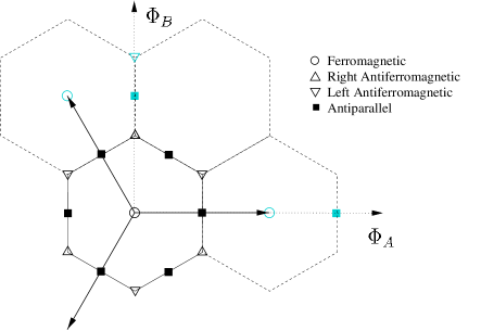
Figure 1: The hexagonal tiling of the $\Phi_{A},\Phi_{B}$ plane. The arrows are the three lattice vectors. The primitive unit cell is solid and copies are dashed. The following fixed points are depicted: (i) the one ferromagnetic (FM) fixed point, (ii) the two antiferromagnetic (AFM) fixed points, and (iii) the three antiparallel (A) fixed points.

Because the the $\phi$ coordinates are $2\pi$ periodic the transformation $\phi_{i}\rightarrow\phi_{i}+2\pi$ does not change the state of the system. This periodicity looks different in the $(\Phi_{A},\Phi_{B})$ plane: the transformation $\phi_{1}\rightarrow\phi_{1}+2\pi$ maps to to a translation in $(\Phi_{A},\Phi_{B})$ space of $({4\pi\over\sqrt{6}},0).$ Adding $2\pi$ to $\phi_{2}$ maps to a translation of ${2\pi\over\sqrt{6}}(-1,\sqrt{3})$ and adding $2\pi$ to $\phi_{3}$ maps to a translation of ${2\pi\over\sqrt{6}}(-1,-\sqrt{3})$ – related by the operator $\mathbf{T},$ these three vectors form the lattice vectors of a hexagonal lattice, see Fig. 1.

Since the $z$’s and $Z$’s are related by the same linear transformation that relates the $\phi$’s and $\Phi$’s, the domain of valid $(Z_{A},Z_{B})$ is hexagonal. One boundary of the hexagon is where spin $1$ is at the north pole, $z_{1}=1,$ since $z_{i}\in[-1,1]$. At that point, $Z_{A}={\sqrt{6}\over 2}.$ When spin $1$ is at the south pole, $z_{1}=-1$ and $Z_{A}=-{\sqrt{6}\over 2}.$ The rest of the boundaries can be found by rotating the $z_{1}=\pm 1$ boundaries by $\pm 120^{\circ}$ in the $(Z_{A},Z_{B})$ plane.

A remaining detail is how the $\Phi,Z$ trajectory appears as a spin passes through a pole. For example, when spin 1 hits the north pole, the the trajectory strikes the boundary of the $(Z_{A},Z_{B})$ hexagon at $Z_{A}={\sqrt{6}\over 2}.$ Although there is no discontinuity in the $z$ or $Z$ coordinates, the $\phi_{1}$ coordinate jumps discontinuously by $\pi$. As seen in $(\Phi_{A},\Phi_{B})$ coordinates, the coordinate $\Phi_{A}$ jumps by $2\pi\over\sqrt{6}.$ As $\dot{z_{1}}$ changes discontinuously at this point, the projection of the trajectory seems to “bounce” off the boundary in $(Z_{A},Z_{B}.)$

III Fixed Points, invariant manifolds and spin waves

III.1 Fixed Points

Certain phenomena of the three spin system, such as fixed points, invariant manifolds and spin waves, can be studied without numerical integration. Section III.1 concerns the fixed points of the three-spin system in which all spins lie in the equatorial plane. Next, Section III.2 describes invariant manifolds of the system – two-dimensional subspaces on which the dynamics are reduced to a single degree of freedom. Finally, Section III.3 develops a linear expansion around the fixed points found in Section III.1 to derive the frequency of spin wave excitations in their phase-space vicinity.

Fixed points are points in phase space where $\dot{\Phi}_{j}=\dot{Z}_{j}=0$ for $j\in\{0,A,B\}$ There are three families of fixed points of the system in which the spins lie in the equatorial plane ($Z_{A}=Z_{B}=0.$) The locations of these fixed points in $(\Phi_{A},\Phi_{B})$ space are plotted on Fig. 1. The ferromagnetic state ($FM$) is the global energy maximum ($E=3$) with all three spins pointing together. The $FM$ state lies at $(0,0)$ in the $(\Phi_{A},\Phi_{B})$ plane. The two antiferromagnetic states ($AFM_{R}$ and $AFM_{L}$) are located at $(0,\pm{2\sqrt{2}\pi\over 3})$ in $(\Phi_{A},\Phi_{B})$ plane and are mirror images of each other. The antiferromagnetic states are global energy minima ($E=-1.5$) with the spins splayed $120^{\circ}$ apart. There are also three antiparallel configurations ($A_{i}$ where $i$ is a spin index $i\in\{1,2,3\}$) where two spins are coaligned while the other spin (spin $i$) points in the opposite direction; here $E=-1.$ $A_{1}$ lies at $(0,\sqrt{2}\pi)$ while $A_{2}$ and $A_{3}$ lie at $(\pm\sqrt{3/2}\pi,\sqrt{1/2}\pi)$ in the $(\Phi_{A},\Phi_{B})$ plane – the operator $\mathbf{T}$ transforms into another by the operator $\mathbf{T},$ a $120^{\circ}$ rotation in the $(\Phi_{A},\Phi_{B})$ plane. The $F$, $AFM$ and $A$ fixed points are fixed points of both the reduced and full systems.

III.2 Invariant Manifolds

If a subspace of the phase space is an invariant manifold, the time evolution of the system will remain in that subspace if its initial state lies in that subspace. As the invariant manifolds of the reduced system are two dimensional, dynamics on the invariant manifolds possess only a single degree of freedom. Therefore, a family of periodic orbits lives on each invariant manifold, which are discussed further in Section V. The three spin system has two kinds of invariant manifold: the stationary spin manifolds and the counterbalanced manifolds. For either kind of manifold, the motion of one spin is different from the other two; with the operator $\mathbf{T}$ one can find three manifolds of each type, related to one another by a $120^{\circ}$ rotation in the $(\Phi_{A},\Phi_{B})$ or $(Z_{A},Z_{B})$ planes.

The $\Phi_{A}=Z_{A}=0$ subspace is one stationary spin manifold. On this manifold, spin 1 lies in the equatorial plane and remains stationary while the other two spins execute roughly circular motions in opposite directions. Motion on the stationary spin manifolds can be modelled with a one-spin system: pointing spin 1 along the $x$-axis, the constraint $\Phi_{A}=Z_{A}=0$ combined with $\sum S_{z}=0$ implies that $S_{3x}=S_{2x},$ $S_{3y}=-S_{2y}$ and ${S}_{3z}=-{S}_{3z}.$ In spin vector form, the reduced Hamiltonian is

$$H_{ss}=2S_{x}+S^{2}_{x}-S^{2}_{y}-(1-\sigma)S^{2}_{z},$$ (11)

where ${\bf S}={\bf S}_{2}.$

The other family of invariant manifolds are the counterbalanced manifolds in which two spins move together in a direction opposite to the other spin; the counterbalanced manifold with spin one the special spin is the subspace $\Phi_{B}=0,Z_{B}=0.$ With the arbitrary choice of $\Phi_{0}=0,$ the following constraints apply: ${\bf S}_{2}={\bf S}_{3}$, $S_{1y}=-2S_{2y}$ and $S_{1z}=-2S_{2z}.$ The remaining constraint, on $S_{2x}$, is determined by the total length constraint $\mid{\bf S}_{1}\mid=1,$ which implies $S_{2x}=\left(+\sqrt{3+S_{1x}^{2}}\right)/2.$ With ${\bf S}={\bf S}_{1}$ the Hamiltonian reduces to

$$H=J\left[1+S_{x}\sqrt{3+S_{x}^{2}}-S_{y}^{2}-S_{z}^{2}+\sigma{3\over 4}S_{z}^{2}\right].$$ (12)

III.3 Spin Waves

Small-energy excitations of a spin system understood in terms of the linearized dynamics around a fixed point are spin waves. This section is a study of the linearized dynamics around the ferromagnetic $(FM)$, antiferromagnetic $(AFM)$ and antiparallel fixed points $(A).$ The term ’spin wave’ is usually used to refer to excitations of a ground state, but the concept remains useful at points such as the antiparallel fixed points which are saddles of the energy function.

The linearization of Eq. (4) near the the ferromagnetic (FM) fixed point is

$$H_{FM}\approx 3-{3\over 2}\left(\Phi_{A}^{2}+\Phi_{B}^{2}\right)-\left({3-\sigma\over 2}\right)\left(Z_{A}^{2}+Z_{B}^{2}\right).$$ (13)

There are two degenerate spin waves with period

$$T_{FM}(\sigma)={2\pi\over\sqrt{3(3-\sigma)}}.$$ (14)

In the case of $\sigma=0.5,$ for which the quantum mechanics have been extensively studied (see Houle et al. (1999)), the analytic value of $T_{FM}=2.294$ agrees with the limit of the periods of all fundamental orbits (computed by numerical integration, see V) as $E\rightarrow 3.$

A similar expansion is possible around either AFM ground state , where $\Phi_{A}$ and $\delta_{B}=\Phi_{B}-{2\sqrt{2}\pi\over 3}$ are small. We obtain

$$H_{AFM}\approx E_{AFM}-{3\over 4}\left(\Phi_{A}^{2}+\delta_{B}^{2}\right)+{1\over 2}\left(Z_{A}^{2}+Z_{B}^{2}\right).$$ (15)

Here there are two degenerate spin waves with period

$$T_{AFM}(\sigma)=\sqrt{2\over 3}{2\pi\over\sqrt{\sigma}}$$ (16)

Approaching the isotropic case, $\sigma\rightarrow 0$, $T_{AFM}$ becomes infinite. This coincides with the exact solution for $\sigma=0$ in which all three spins precess around the total spin vector Magyari et al. (1987) at a rate proportional to the length of the total spin vector: at $AFM$, the total spin and the rate of spin precession are both zero. When $\sigma=0.5$, the periods of all fundamental orbits converge to $T_{AFM}=7.255$ as $E\rightarrow-1.5$ as predicted by Eq. (16). As the spin wave frequency drops to zero, the zero point energy of the quantum ground state also drops to zero, converging on the classical ground state energy as is observed in Houle et al. (1999).

Although $A_{i}$ is a saddle point rather than a ground state, it is still possible to linearize the Hamiltonian in its vicinity. Let $\Phi_{B}$ and $\delta A$ be small, where $\delta A=\Phi_{A}-\bar{\Phi}_{A},$ and $\bar{\Phi}_{A}=-\sqrt{2/3}\pi.$ Then,

$$H_{A} \approx E_{A}+\left[\left({1\over 6}+{\sigma\over 2}\right)Z_{A}^{2}+{3\over 2}\delta_{A}\right]$$ (17)

$$\;\;\;\;\;\;\;\;\;\;\;\;\;\;\;-\left[{(1-\sigma)\over 2}Z_{B}^{2}+{\Phi_{B}^{2}\over 2}\right].$$

The first set of terms in Eq. (17) depends on $Z_{A}$ and $\Phi_{A}$ and the second set depends on $Z_{B}$ and $\Phi_{B}.$ The first set in Eq. (17) describes positive energy spin waves that live on the $Z_{B}=\Phi_{B}=0$ counterbalanced manifold with period

$$T_{A,c}(\sigma)={2\pi\over\sqrt{1+3\sigma}},$$ (18)

which is $T_{A,c}=3.975$ when $\sigma=0.5.$ The second set describes negative energy spin waves that live on the $Z_{A}=\Phi_{A}=0$ stationary spin manifold with period

$$T_{A,ss}(\sigma)={2\pi\over\sqrt{1-\sigma}},$$ (19)

which is $T_{A,ss}=8.885$ when $\sigma=0.5.$ Corners of the counterbalanced and stationary spin manifolds touch at right angles at $A.$ We will later take advantage of this to compute the stability properties of the stationary spin and counterbalanced orbits in Section V.2.

IV The topology of the energy surface

Unlike the canonical cases of two-degree of freedom Hamiltonian dynamics, such as the Anisotropic Kepler Problem (AKP) and the Henon-Heiles Hamiltonian, the three-spin system exhibits nontrivial changes in the topology of the energy surface at certain energies. There are three transition energies: (i) the coalescence energy $E_{c}(\sigma);$ (ii) the antiparallel energy $E_{A}=-1;$ and (iii) the polar energy $E_{p}(\sigma)$. Fig. 3 depicts the transition energies as a function of $\sigma$ while Fig. 4 illustrates the topology changes for $\sigma=0.5$. As we increase energy from the ground state $E=-1.5$, transition (i) always occurs first. If $0<\sigma<2/3$, transition (iii) occurs before transition (ii), otherwise when ${2/3}<\sigma<1$ (ii) occurs before (iii).

IV.1 The coalescence transition

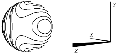
Figure 5: The trajectory of a moving spin on the stationary spin manifold, for $\sigma=0.5.$ The well around the negative z-axis is the antiparallel fixed point, while the wells above and below it are the two antiferromagnetic fixed points. (The FM fixed point is on the positive x-axis and is on the hidden side of the sphere.) The separatrix between orbits centered on the AFM fixed points those centered around the antiparallel fixed points occurs at energy $E_{c}$ (see Eq. (21).)

At low energies (near the AFM fixed points) an energy barrier separates the two antiferromagnetic ground states. Therefore, the energy surface is composed of two disconnected parts. Those parts become connected when $E=E_{c}(\sigma).$ Using polar coordinates, ${\bf S}=(\sin\theta\cos\phi,\sin\theta\sin\phi,\cos\theta),$ the surfaces first touch at the saddle points on the $\phi=0$ line on Fig. 5 (one is hidden behind the sphere.) Thus, $E_{c}(\sigma)$ is found by considering Eq. (11), the single-spin Hamiltonian for the stationary-spin manifold. The saddle lies on the $\phi=0$ line, at the point where ${\partial H/\partial\theta}=0$, or

$$\sin\theta={1\over 2-\sigma}.$$ (20)

Substituting this back into Eq. (11), the saddle-point energy is

$$E_{c}(\sigma)={3-3\sigma+\sigma^{2}\over\sigma-2}.$$ (21)

The coalescence occurs between (a) and (b) in Fig. 4. An interesting quantum manfestation of the coalescence transition was observed in Houle et al. (1999), the tunnel splitting of quantum levels as $E_{c}$ is approached from below.

IV.2 The antiparallel transition

At $E_{c}$, a set of necks come into existence that connect the two lobes of the energy surface that were disconnected at energies below $E_{c}$ (See Fig. 4b) when $E=-1$ these necks fuse, changing the connectedness of the energy surface again (See Fig. 4c.) This is the antiparallel transition – the antiparallel fixed point $A_{1}$ (see Section III.1) lies in the center of the large hole in Fig. 4b. Two families of periodic orbits disappear at this transition, including one branch of stationary spin orbits approaching from $E<-1$ as well as the counterbalanced orbits approaching from $E>-1.$ (One aspect of Fig. 4b is deceptive. Being a three-dimensional cut out of a four-dimensioanl space, it fails to show two other pairs of connecting necks that surround the $A_{2}$ and $A_{3}$ antiparallel fixed points – for a total of six necks.)

IV.3 The polar transition

The system attains extreme energies (both minimum and maximum) only when the spins lie in the equatorial plane. As a result, there is both a minimum and a maximum energy at which one spin can point at a pole, which is a saddle point in the full phase space. These are the upper and lower polar transition energies – these thresholds are found by pointing one spin, say spin 1, at the north pole and finding the maximum and minimum energy configurations. Setting $Z_{A}=\sqrt{3/2},$ in Eq. (4-6) we get

$$H = -{(1-\sigma)\over 2}\left({3\over 2}+Z_{B}^{2}\right)$$ (22)

$$\;\;\;\;\;+{1\over 4}\sqrt{9-20Z_{B}^{2}+4Z_{B}^{4}}\cos\left(2\Phi_{B}\right).$$

which has a maximum at $H_{max}={3\over 4}\sigma$ and a minimum at $H_{min}={3\over 4}\sigma-{3\over 2}.$ The polar transition occurs between panels (c) and (d) in Fig. 4: at this point the energy surfaces touch the enclosing hexagonal prism, forming a network of necks connecting the energy surface to itself.

IV.4 The classical density of states

Changes in the topology of the surface section have an interesting effect on the classical and quantum densities of states. The weighted area of the energy surface,

$$\rho_{c}(E)=\int d\Phi_{A}d\Phi_{B}dZ_{A}dZ_{B}\delta(E-H(H,E))$$ (23)

is the classical density of states, since it is proportional to the quantum density of states. endnote1 Fig. 6 is a plot of the classical density of states for the reduced system as a function in energy. We observe two interesting features: first, a discontinuity in the slope of $\sigma_{c}(E)$ at the coalescence transition (This is (a) in Fig. 6.) Second, the density of states is apparently flat between the lower polar transition $E_{p}(\sigma)$ and the antiparallel transition – although we don’t have an analytic understanding of the flat spot, numerical evidence suggests that it is exactly flat.

V Fundamental Periodic Orbits and Global dynamics

This section presents the main results we’ve determined from numerical integration of the equations of motion: a map of the fundamental periodic orbits of the three-spin system for and Poincaré sections depicting the global dynamics of the system for $\sigma=0.5$. Like any chaotic system, the three spin system has an infinite number of periodic orbits. However, a few short period orbits form the skeleton of the system’s dynamics. Four of these are known; the stationary-spin orbit, the counterbalanced orbit, the three-phase and the unbalanced orbit. Fig. 7 plots the energy-time curves of the four orbits for $\sigma=0.5.$ (Spin trajectories for the four orbit types are visualized in Fig. 1 of Houle et al. (1999))

Sections V.1 - V.3 discuss the stationary-spin, counterbalanced, three-phase and unbalanced orbits respectively. Section V.5 and V.6 discuss global dynamics near the ferromagnetic ($E\rightarrow 3$) and antiferromagnetic ($E\rightarrow-1.5$) ends. Section V.7 points out how symmetries of the Hamiltonian manifest in its classical dynamics.

V.1 Stationary spin orbits

The stationary spin orbits are simple to study because any point on a stationary spin invariant manifold (see Section III.2) lies on a stationary spin orbit. As there are three stationary spin manifolds, there are three families of stationary spin orbits related by symmetry.

For a stationary spin orbit, one spin (say, spin 1) is stationary in the equatorial plane, while the other two spins move in distorted circles, $180^{\circ}$ out of phase. Fig. 5 is a plot of the trajectories of one of the moving spins, based on the single-spin Hamiltonian Eq. (11). In the range $-1<E<3,$ each family of stationary spin orbits has a single branch; trajectories on the single-spin sphere are concentric distorted circles centered around the FM fixed point. Between $E=-1$ and $E=E_{c}$, two branches of periodic orbits exist: the outer branch, still centered around the $FM$ fixed point, and the inner branch, centered around the $A$ fixed point. Below the coalescence energy $E_{c}(\sigma)$, the orbits reorganize into a different pair of branches (left and right), one centered around each antiferromagnetic ground state.

The stationary spin orbit runs along the $Z_{A}=0$ seam on the slice of the energy surface visualized in Fig. 4. Fig. 4d and c represent the case where $E>-1$ and only one branch of the orbit exists. In Fig. 4b, the outer branch runs along the outside of the surface while the inner branch rungs along the inside of the hole in the surface. Finally in Fig. 4a, left and right branches of the the stationary spin orbit exist on two separate lobes of the energy surface.

The energy-time curve for the stationary spin orbits is seen in Fig. 7. Although one would expect that the periods of the left and right branches in the $E<E_{c}$ regime are the same (because they are related by reflection symmetry,) it’s a bit surprising that the period $T(E)$ of the inner and outer branches in the $E_{c}<E<-1$ is also the same. Since the coalescence separatrix intersects the stationary-spin manifold, the period of the stationary spin orbits goes to infinity as $E\rightarrow E_{c}$ from either side, with an observable effect on the quantum mechanical orbit spectrum.Houle et al. (1999)

In the case of $\sigma=0.5,$ the stationary spin orbit is unstable for $E>-1.$ For $-1<E<E_{c},$ the inner branch of the stationary spin orbit is stable and the outer branch is unstable. The left and right branches are stable as $E\rightarrow-1.5$ but become unstable as the energy increases and chaos becomes widespread (the orbit does momentarily regain its stability near $E=-1.22.$) Fig. 8 is a plot of the stability parameter $\rho=\lambda+\lambda^{-1}$ versus energy for $E<-1,$ where $\lambda$ and $\lambda^{-1}$ are eigenvalues of the transverse stability matrix; $|\rho|<2$ for a stable orbit and and $|\rho|>2$ an unstable orbit. Lichtenberg and Lieberman (1992)

V.2 Counterbalanced orbits

The counterbalanced orbit family is also easy to study because, like the stationary spin family, it lives on an invariant manifold. Counterbalanced orbits exist only in the range $E>-1,$ and at least for $0<\sigma<2,$ the counterbalanced orbit is always stable. As is the case for counterbalanced manifolds, there are three counterbalanced orbits related by the symmetry $\mathbf{T}.$

The spin wave analysis of Section III.3 can be applied to the stability properties of the inner branch stationary spin and counterbalanced orbits in the limit $E\rightarrow 1$. A counterbalanced orbit (approaching from $E>-1$) and the inner branch of a stationary spin orbit touch at each antiparallel fixed point. Using the linearization around the antiparallel fixed point Eq. (17), we can establish that both orbits are stable, and compute the limiting value of the stability exponent $\rho$ at $E\rightarrow-1$ for both orbits.

Because there are two distinct frequencies in the linearized dynamics around the antiparallel fixed point, Eq. (17), dynamics in the vicinity of the antiparallel fixed point are structurally stable and, for close enough energies, should be similar to the linearized behavior. Focusing attention on the counterbalanced orbit, the degree of freedom orthogonal to the counterbalanced orbit is the stationary spin orbit – therefore the counterbalanced orbit is stable as $E\rightarrow-1.$ In one circuit of the counterbalanced spin orbit, a slightly displaced trajectory winds around the orbit at the frequency of the stationary spin spin wave. The winding number is the ratio of the periods of the two orbits, or

$$\theta=2\pi{T_{c}\over T_{ss}}=\sqrt{{1-\sigma}\over{1+3\sigma}}.$$ (24)

For $\sigma={1\over 2},\theta={2\pi\over\sqrt{5}}.$ The stability parameter $\rho=2\cos\theta$ equals $-1.891,$ and agrees with the result obtained by numerical integration (see Fig. 9). Repeating this analysis for the stationary spin orbit, we obtain $\rho\rightarrow 0.175$ in agreement with Fig. 8.

V.3 Three phase orbits

The three phase orbits do not lie on an invariant manifold and thus have richer behavior than the previous two families of orbits. Unlike the stationary spin and counterbalanced orbits for which $<\!\!\dot{\Phi}_{0}\!\!>=0,$ three phase orbits can exhibit precession, a secular trend in $\Phi_{0}$ and therefore can be periodic orbits of the reduced system but not the full system. The three phase orbit undergoes a pitchfork birfucation at transition energy $E_{b}$ ($E_{b}\approx-0.75$ for $\sigma=0.5$.) Above $E_{b},$ a single branch of non-precessing orbits exists, but below the bifurcation three branches of three phase orbits exist: a non-precessing unstable orbit and two stable orbits for which $<\!\!\dot{\Phi}_{0}\!\!>\neq 0$ with opposite signs. This transition is visible on curve (c) of Fig. 7. The unstable orbit exists for a small energy below $E_{b}$ but soon disappears when the spin trajectory intercepts the poles of the spin spheres.

The three-phase orbits are so called because, in three-phase orbits, the spins each execute an identical circuit around a distorted circle, each $120^{\circ}$ out of phase – much like the currents used in three-phase AC power transmission. The multiplicity of the three-phase orbit is different from the previous two: Above $E_{b}$ there are two three-phase orbits, one in which the spins rotate clockwise and another with counterclockwise rotation. Below $E_{b}$ and the demise of the nonprecessing orbit, there are a total of four: each AFM ground state has it’s own pair, one member of which has $<\!\!\dot{\Phi}_{0}\!\!>$ positive and the other $<\!\!\dot{\Phi}_{0}\!\!>$ negative. Fig. 10 is a plot of the per-orbit precession rate of the three-phase orbit below the pitchfork bifurcation; note that the precession rate converges on $2\pi$ (effectively zero) as $E\rightarrow-1.5.$

The three phase family is more difficult to study than the previous two, because we must search the energy surface for it. It’s still quite straightforward, for as seen in Sections V.5 and V.6 the three spin orbit lies on the $Z_{B}=0$ line of the $\Phi_{A}=0$ surface of section and can be found by a one-dimensional search. The stability exponent $\rho$ of the three-spin orbit can be seen in Fig. 11.

V.4 Unbalanced Orbits

The unbalanced orbits, a family of unstable periodic orbits, exist between $E=-1.5$ and $E=E_{p}.$ Unbalanced orbits do not lie on a symmetric manifold and do not precess. The unbalanced family corresponds with the unstable fundamental periodic orbit of the Hénon-Heiles problem near its ground state – in the $(\Phi_{A},\Phi_{B})$ plane the projection of an unbalanced orbits is roughly a parabola that does not pass through the projection of the AFM fixed point. Like the first two orbit families, the behavior of one spin in the unbalanced orbit is different from the other two; therefore there are three unbalanced orbits for each of the two AFM fixed points, for a total of six unbalanced orbits. At low energies, the odd spin moves along a closed curve in $(\phi,\theta)$ space while the other two spins move along open curves which are dented on one corner and are mirror images of one another. One unbalanced orbit lies on the line $Z_{B}=0$ line of the $Z_{A}=0$ surface of section.

The unbalanced orbit disappears at the polar transition, at which point the trajectory of the odd spin grazes the poles, touching the holes that appear between Fig. 4c and 4d.

V.5 Dynamics near the ferromagnetic end

The periodic orbits are the “skeleton” of the dynamics of a system: to understand the “flesh” requires the global view obtained through Poincaré sections. Choosing a good trigger plane for our section was a matter of studying the projection of orbits in the $(\Phi_{A},\Phi_{B})$ plane: to ensure that all fundamental orbits appear in the Poincaré section, our criteria were that: (i) all orbits crossed the trigger plane, and (ii) no orbits were confined to the trigger plane. $\Phi_{A}+\Phi_{B}=0$ satisfied both requirements.

($\Phi,Z$) coordinates improve the quality of our Poincaré sections compared to previous works on the three-spin system. Nakamura and Bishop (1986) In previous works, Poincaré sections were taken with trigger $dS_{1z}/dt=0$ and projected on the $S_{x}$ and $S_{y}$ planes. When this is done, the collective precession of the three spins cannot be visually separated from more interesting degrees of freedom. Although the concentric loops of KAM tori can be seen in the figures of Nakamura and Bishop (1986) when the trajectories on the tori are non-precessing, they are superimposed by random dots from precessing chaotic trajectories. Worse, at energies close to the antiferromagnetic ground state ($E=-1.5$), trajectories on KAM tori themselves precess, destroying their image. As a result, the sections of Nakamura and Bishop (1986) had limited utility as a map of the dynamics of the three spin system and had to be supplemented with power spectra of the classical trajectories to determine if trajectories were regular or chaotic.

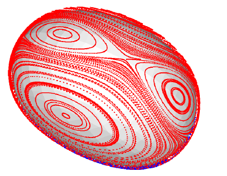
Figure 12: Poincaré section at $\sigma=0.5,E=2.0$ with a $\Phi_{A}+\Phi_{B}=0$ trigger: point (a) is a stationary spin orbit, point (b) is a counterbalanced orbit, and point (c) is a three-phase orbit. The energy surface is approximately an oblate spheroid with stationary spin and counterbalanced orbits on the equator on which $\Phi_{B}=0;$ the back side of the surface is hidden. Just behind the equator is the other three-spin orbit for which the spins rotate opposite the direction of the visible three-spin orbit. Throughout most of the visible hemisphere, orbits cross the section traveling in the positive direction ($\dot{\Phi}_{A}>0$); on the invisible hemisphere, the picture is mirror-reflected across the “terminator” for orbits crossing in the negative direction.

Fig. 12 is a surface of section using the $\Phi_{A}+\Phi_{B}=0$ trigger which we produced using a method of visualizing Poincaré sections for two degree of freedom systems in three dimensional space described in Appendix B. Fig. 12 is a single image of a simulated 3 dimensional object which can be interactively rotated and viewed from arbitrary positions. The dark opaque object is the $E=2.05$ energy surface, which is approximately an oblate spheroid with the $(Z_{A},Z_{B})$ plane passing through the equator. Over that surface is plotted cloud of dots which are the intersections of $E=2.0$ trajectories with the surface of section.

All of the fundamental periodic orbits intersect the surface of section in two places, once passing through the surface of section in the positive direction ($\dot{\Phi}_{A}>0$) and once in the negative direction ($\dot{\Phi}_{A}>0$.) Just on the lower visible edge of the energy surface is a sort of terminator which divides trajectories that cross the surface of section in the positive and negative directions; this curve is not quite a geodesic but it does divide the energy surface into two approximate hemispheres. The intersections of the stationary-spin and counterbalanced orbits with the surface of section form a ring of 12 fixed points lying in the $(Z_{A},Z_{B})$ plane with exact 12-fold symmetry while the two three-phase orbits cross the surface of section away from the plane.

The nature of KAM tori in the ferromagnetic limit $E\rightarrow 3$ is visible in Fig. 12. A concentric family of KAM tori exist around each counterbalanced orbit, and families of tori also exist centered around the three-phase orbits. Stationary spin orbits lie on the separatrix which divides counterbalanced tori from three spin tori. As energy is lowered, this separatrix is the first place where tori break and chaos is observed.

V.6 Dynamics near the antiferromagnetic end

To study the dynamics of the three-spin system near the antiferromagnetic end, $E\rightarrow-{3\over 2}$ we chose $\Phi_{A}=0$ as a trigger. Although this violates criterion (ii) of Section V.5, we gain the advantage that this trigger plane extends from the lowest to the highest energies and crosses both antiferromagnetic fixed points. The practical disadvantage is that a stationary spin orbit exists on the $\Phi_{A}=0$ line, and appears as a curve on the Poincaré section rather than a point, but this does not terribly complicate the interpretation of the section.

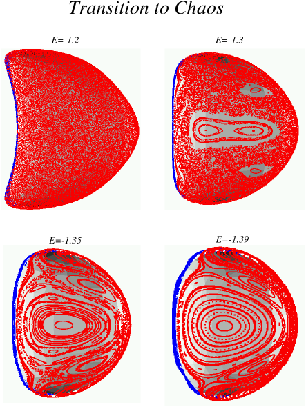
Figure 13: The transition to chaos at the antiferromagnetic end ($E\to-1.5$) with $\sigma=0.5.$ Shown is one of the two lobes from Fig. 4. See Fig. 14 to determine which orbits are which.

Fig. 13 illustrates the transition to chaos in the antiferromagnetic regime with $\sigma=0.5$. At $E=-1.39$ (see Fig. 14) most tori are unbroken and motion is primarily regular. By $E=-1.35$ chaos is becoming noticeable in separatrix regions, and by $E=-1.3$ chaos is widespread. At $E=-1.2$ no islands of regular motion are obvious. However, we know that regular islands do exist because the inner branch of the stationary spin orbit is stable at some energies in this regime (See section V.) The transition to chaos on the antiferromagnetic side has been observed previously Nakamura and Bishop (1986) in the same energy range.

V.7 Symmetry and dynamics

Because the Hamiltonian (4) is threefold symmetric around the antiferromagnetic fixed points, (see Section II.2) the low energy behavior of the three spin system falls into the same universality class as the well-known Hénon-Heiles system with Hamiltonian Gutzwiller (1990)

$$H={1\over 2m}(p_{x}^{2}+p_{y}^{2})+{m\omega^{2}\over 2}(x^{2}+y^{2})+\lambda(x^{2}y-y^{3}/3).$$ (25)

This can be seen in Fig. 14, which looks remarkably like Poincaré  sections of the Hénon-Heiles system. Gustavson (1966)

Symmetries around a fixed point determine many properties of the dynamics of a system in its vicinity including the nature of the fundamental orbits, the global geometry of trajectories in phase space, and degeneracies in orbit frequencies. Threefold rotation symmetry around the antiferromagnetic fixed point ensures that the periodic orbits and KAM tori near one AFM fixed point can be mapped 1-1 to those in Hénon-Heiles, but it also guarantees that the frequencies of all periodic orbits converge in the $E\rightarrow-1.5$ limit: if we perform a Taylor series expansion of the Hamiltonian at the fixed point (as in Eq. (15)) the only quadratic term compatible with threefold rotation symmetry is that with circular symmetry in the $(\Phi_{A},\delta_{B})$ and $(Z_{A},Z_{B})$ planes.

The three-spin system exhibits a six-fold rotation symmetry near the FM limit which is responsible for a different orbit and torus geometry in the $E\rightarrow 3$ limit which is probably generic for Hamiltonian fixed points with sixfold symmetry. With six-fold symmetry, the first and second derivatives of the time-energy curves are the same for all fundamental orbits at $E=3;$ as a result, the periods of orbits are remarkably degenerate for a large range in energy (see Fig. 7.)

VI Conclusion

This paper is a detailed analysis of the classical dynamics of the three spin cluster with Hamiltonian Eq. (1); many of the features we find are connected with quantum phenomena in the accompanying paper Houle et al. (1999). One class of phenomena are connected with changes in the topology of the energy surface (see Section IV) which occur as a function of energy: if we make a plot of quantum energy levels as a function of $\sigma,$ shown in Fig. 5 of Houle et al. (1999), we observe a tunnel splitting as pairs of near-degenerate levels (at $E<E_{c}(\sigma)$) cross the $E_{c}(\sigma)$ curve (see Eq. (21).) This is caused by tunneling between quantum states localized on the two disconnected parts of the energy surface. A second phenomenon related to the topology of the energy surface is that the classical and quantum densities of states are apparently constant as a function of energy for $E_{c}(\sigma)<E<-1$ (see Fig. 4 of Houle et al. (1999) and Section IV.4 of this paper.)

Our analysis of fundamental periodic orbits in Section IV also has significance for the quantum problem. The Gutzwiller trace formula Gutzwiller (1990) predicts that classical periodic orbits cause oscillations in the density of states. In Houle et al. (1999) we observed these oscillations by applying spectral analysis to the quantum density of states. (see Fig. 3 of Houle et al. (1999).)

Some technical aspects of the work presented in this paper are interesting. First, the change of coordinates that presented in Section II.1 enables us to understand the three-spin cluster better than previous studies Nakamura et al. (1985) Nakamura (1993) as we take advantage of the clusters conservation of total $S_{z}$ to reduce the dynamics to a tractable two-degree of freedom system. Second, our use of three-dimensional visualization for visualizing the energy surface and Poincaré sections clarifies interpretation of Poincaré sections when the topology of the energy surface is complicated. Even in situations where the topology is simple (such as is discussed in Section V.5,) three-dimensional visualization hides fewer symmetries of system than the customary two-dimensional projection and eliminates the confusion caused when two sheets of the energy surface are projected on top of one another. This method is described further in Appendix B

The three-spin cluster has similiaries to certain well-studied systems. Our system has features in common with the well-known Anisotropic Kepler Problem (AKP). Gutzwiller (1990). Like the AKP, total angular momentum around the z-axis $\sum S_{i}^{z}$ is conserved, leaving two nontrivial degrees of freedom. Both the AKP and Eq. (1) have a single parameter ($\sigma$ in the case of our system) and are nonintegrable for all values of the parameter save one ($\sigma=0$ in our case.) In both systems, all three classical frequencies are identical in the integrable case. For the AKP, the integrable case is the ancient Kepler problem in which all trajectories are closed ellipses. In our problem, in the integrable case $(\sigma=0),$ all three spins precess around the total spin vector $\sum_{i}{\bf S}_{i}$ at a rate proportional to the length of the total spin vector. Magyari et al. (1987) Our system is different from the AKP in a number of ways. First, the AKP is highly chaotic throughout the parameter space in which is has been studied Gutzwiller (1990) (The first stable periodic orbit was found after the AKP had been studied for 14 years. Broucke (1985)) Our system, on the other hand, shows highly regular behavior in much of the parameter space (For instance, when $E>2$ in the $\sigma=0.5$ case) as well as irregular behavior in other areas (For instance, $\sigma=0.5$ and $E\approx-1.2.$) Thus the elegant application of symbolic dynamics to the AKP Gutzwiller (1990) is not possible for our system.

Another connection between the three-spin cluster and a well-studied system is the similarity between the dynamics of the three-spin cluster in the antiferromagnetic limit and the Hénon-Heiles problem. Gustavson (1966); Hénon and Heiles (1964) The connection here is most obvious in the surface of section shown in Fig. 14 and occurs because the three-spin cluster has a three-fold rotational symmetry around the antiferromagnetic ground states similar to the symmetry of the Hénon-Heiles problem.

In this work we have gotten a more intimate understanding of a nonintegrable spin cluster than has been previously available supporting the work described in Houle et al. (1999), which establishes that periodic orbit theory can be applied to spin. This work was funded by NSF Grant DMR-9612304, using computer facilities of the Cornell Center for Materials Research supported by NSF grant DMR-9632275. We would like to thank Masa Tsuchiya, Jim Sethna, and Greg Ezra for interesting discussions.

Appendix A Numerical Integration in $\Phi,Z$ coordinates

An important decision in the numerical study of the three spin problem is the choice of variables to used to integrate the equation of motion. This choice affects the speed, complexity and reliability of integration as well as the range of Poincaré sections that can be easily taken.

Our ODE integrator library was written in Java and evolved from the software used for the results published in Houle (1997). For both vector components and $(\Phi,Z)$ coordinates we used adaptive fifth-order Runge-Kutta integration based on the code from Press et al. (1992) although our system allows the use of different integrators such as fourth-order fixed Runge-Kutta for testing. endnote2

In the early phase of this work we integrated the spin vector components $(S_{x},S_{y},S_{z})$ of the individual spins. The vector component representation has several advantages: the software requirements are simple and it’s straightforward to write a general routine for evaluating the equations of motion for any spin Hamiltonian which is polynomial in $S_{x}$, $S_{y}$ and $S_{z}.$ Spin vector coordinates are also free of obnoxious singularities. However, the need to isolate the overall precession of the spins from more interesting motions led us to integrate the system in $(\Phi,Z)$ coordinates so we could easily set Poincaré sections in the $\Phi$-space. (the rationale for setting triggers in $\Phi$ space is discussed in Section V.5.)

Although the transformation $(\phi,z)\rightarrow(\Phi,Z)$ is a straightforward linear transformation, the need to use inverse trigonometric functions to convert ${\bf S}$ into $(\phi,z)$ adds overhead and, more seriously, additional complexity to deal with branch cuts. (Numerical algorithms that work with branch cuts, particularly involving square roots, are difficult to design. Failure modes caused by roundoff error with a probability of $10^{-6}$ per dynamical timescale are a major complication for a program that calculates thousands of trajectories.) Simple strategies for disambiguating branch cuts that do not introduce an error-prone memory between steps lose valuable topological information. If, for instance, $\Phi_{0}$ is computed from some manipulation of the ${\bf S}_{i}$ components, and, say, is always in the range $0<\Phi_{0}<{4\pi\sqrt{3}}$ it isn’t as easy to determine the net precession (secular trend of $\Phi_{0}$) of a periodic orbit as it would be if $\Phi_{0}$ were integrated directly.

We performed all of the integrations in this work in $(\Phi,Z)$ coordinates, with equations of motion derived from Eq. (4). The main difficulty we had is that the integration can fail on a trajectory on which a spin passes through a pole; this is not a failing of the $(\Phi,Z)$ coordinates as much as of the $(\phi,z)$ coordinates. As spin $i$ passes close to the pole, the singularity in the mapping from $(\phi_{i},z_{i})\rightarrow{\bf S}_{i}$ forces $\dot{\phi}_{i}\rightarrow\infty.$ If the trajectory misses the pole by more than $1e-6$ in the $z$ axis when using double precision math, the primary consequence is that the adaptive step size integrator reduces the time step and integration is slowed. If the trajectory passes much closer to the pole, however, no step size may have a sufficiently small error estimate and the adaptive step size algorithm will fail. Although it would be possible to avoid this problem by either switching to spin vector coordinates when the trajectory passes close to the pole or by adding more intelligence (and possibly bugs) to the adaptive step size algorithm, in practice it affects a small enough volume of phase space that it only manifests when investigating trajectories specifically chosen to pass near a pole.

Sometimes it is necessary to work with ($\Phi_{A}$,$\Phi_{B}$) normalized to the unit hexagon, for instance, to set a Poincaré section trigger on $\Phi_{A}=0.$ At energies above the upper polar transition and below the lower polar transition (see Section IV) this is not necessary because the trajectory does not wander long distances in the ($\Phi_{A}$,$\Phi_{B}$) plane. For some time this prevented us from taking Poincaré sections in the region between the two transitions, since the trajectory would eventually wander far from the trigger plane. To solve this, we found an algorithm for mapping $(\Phi_{A},\Phi_{B})$ back to the unit hexagon: first, (i) use the modulus function to map points into the primitive cell of the hexagonal lattice, a rhombus. Then, (ii) apply a unit vector translation to those points that fall on corners of the rhombus outside the unit hex to bring them into the unit hex.

Appendix B Solid Poincaré Sections

In the process of studying the three spin problem, we found conventional methods of drawing Poincaré  sections inadequate and improved upon them by developing a method for rendering Poincaré  sections in three-dimensional space. This greatly simplified the interpretation of Poincaré  sections for our system. Although not all systems pose as serious technical problems as ours, we believe that this method clarifies the geometry of Poincaré sections and can simplify the presentation of Poincaré sections to audiences which are not specialized in dynamics. The techniques described in this appendix were used to generate Fig. 4, Fig. 12 and Fig. 13.

For Hamiltonian systems with two degrees of freedom, the intersection of the energy surface with the surface of section is a two-dimensional surface embedded in a three-dimensional space (the surface of section). Often, this intersection has the topology of a sphere – this is true of the Hénon-Heiles system as well as for the three spin systems above the upper polar threshold and below the coalescence energy $E_{c}(\sigma).$ The trajectory crosses the surface of section in two directions, which we will call the positive and negative directions. Over part of the sphere, the trajectory crosses in the positive direction and over the rest of the sphere, the trajectory crosses in the negative direction. In between there is a seam over which the trajectory is tangent to the surface of section.

Difficulties arise when plotting the intersection of trajectories with the surface of section even when the topology is simple. To take a specific example, consider the case of the three spin problem with $\sigma=0.5$ and $E=-2$ with the trigger on $\Phi_{A}+\Phi_{B}=0.$ A reasonable set of $(x,y,z)$ variables for this problem is $(x,y,z)=(Z_{A},Z_{B},\Phi_{A}).$ Conventional choices of projection are $(x,y)$ which would overlap the two distinct three phase orbits and place the stationary spin orbits on the edge of the plot, or $(x,z)$ which obscures the symmetry of the stationary spin and counterbalanced orbits seen in the $(x,y)$ plane.

While writing the paper Houle (1997) we began development of a set of Java class libraries for integrating differential equations and taking Poincaré  sections. Interchangeable trigger modules are connected to the differential equation integrator, allowing the user to set a triggering criteria for surface of section. When the surface is crossed, we solve for the crossing time by varying the integration step $\delta t$ and solving for the value of $\delta t$ that intersects the section by the Newton-Raphson method. (We also tried the method of method of Hénon Hénon (1982) in which a change of variable is made to make the trigger coordinate become a time coordinate – we found that performance of our method and Hénon’s method is similar, but ours was more robust) We primarily integrate with an adaptive fifth-order Runge-Kutta implementation, but the design of our program allows us to replace our integrator with another fixed or adaptive step algorithm.

One component of a 3-d Poincaré  section is a rendering of the energy surface. For an arbitrary system, the energy surface can be rendered by treating it as an implicit function;

$$E(x,y,z)=E_{0}$$ (26)

this sort of surface can be rendered using ray-tracing techniques, or can be rendered in a primitive manner by dividing the 3-space into voxels and coloring in cubes which are above or below a threshold value. A better method is to generate a polygonal mesh with Bloomenthal’s algorithm Bloomenthal (1988). The relative merits of various methods for polygonizing a mesh are discussed in Glassner (1990). For a uniform mesh (not adaptively sampled), Bloomenthal’s algorithm is equivalent to a table-driven method known as Marching Cubes Lorensen and Cline (1987). We can compute a mesh for our system in under 20 seconds and 2 megabytes of storage, and this time could be reduced by the use of Marching Cubes. The resulting mesh can be rendered with a standard 3-d system, either an interactive system such as as OpenGL or VRML or an off-line system such as POVRay or Renderman.

The generation of the actual Poincaré sections is quite straightforward. We merely plot a set of (x,y,z) points when the trajectory intersects the surface of section. The last problem is determining initial conditions for injection. In some cases we wish to interactively choose injection points, in which case it’s necessary to translate a hand-chosen injection point in screen cordinates into into a point one on the energy surface; this way, in an interactive 3-d environment, a user can click on the energy surface to set an injection point. For most cases, we prefer to have the computer automatically generate Poincaré sections, choosing injection points that reveal all major phase space structures. To accomplish this, our program divides the surface of section into voxels (tiny cubes) and inspects the value of the energy at the corners of the cubes to find which cubes intersect the energy surface. Next, the program scans the surface, ensuring at least one trajectory either originates in or passes through each voxel that contains part of the energy surface. To inject in a voxel, our program computes the gradient of the Hamiltonian at the center of the voxel and precisely locates the energy surface by a Newton search along the line of fastest change in energy. It then marks that voxel as filled. The trajectory is then evolved forward in time for a fixed number of intersections: at each intersection, the containing voxel is set as filled. The program continues to find voxels which are not filled and injects into them until all voxels are filled.

Although the energy surfaces are interesting in themselves for systems with topology changes (such as the three spin system), they are also essential for interpreting solid Poincaré sections. To make a solid Poincaré section we render a cloud of dots in three-dimensional space at the points where trajectories intersect the surface of section. The resulting dot cloud is transparent and is difficult to make sense of without an opaque object underneath it. Several factors conspire to confuse the eye. For instance, a part of a dot cloud that is further from the viewer is made visually denser by perspective which makes it appear heavier and more solid to the viewer – causing the viewer to conclude that the distant part of the dot cloud is closer. An opaque rendering of the energy surface eliminates the confusion caused when images of the energy surface overlap.

Because integrating differential equations is slow, it takes about two hours to compute our Poincaré sections. Because the calculation can be broken into a a number of mainly unrelated calculations, parallelizing the calculation across multiple processors on an SMP machine or a cluster of computers would be straightforward and worthwhile.

A complicated aspect of the three-spin problem is the hexagonal tiling of the phase space. This introduced two difficulties which required special solutions. We implemented these solutions using object-oriented techniques to replace general-purpose classes with specialized subclasses. First, the 3-space $(Z_{A},Z_{B},\Phi_{A})$ is bounded by the points at which the spins touch the north pole. The volume inside this boundary is a hexagonal prism (See Section II.3 and Fig. 4) Using a cubical grid to represent a non-cubical domain forced us to keep track of which points were inside the hexagonal prism and which were outside. Not only was this difficult and slow, but the irregular pixilation of the boundary confused both the surface-constructing algorithms and the eye of the viewer, resulting in surfaces with a jagged, serrated appearance. We solved the problem by replacing the Java class responsible for mapping integer voxel numbers to ($x,y,z$) coordinates with one that smoothly maps a cubic grid on an integer lattice to a hexagonal prism. All sample points fell within the allowed range. We headed off numerical problems caused by square roots in the energy function by multiplying x and y coordinates by $1-10^{-13}$ before computing the energy.

At energies between the upper and lower polar thresholds, another set of problems arises. Here, the projection of a trajectory in ($\Phi_{A},\Phi_{B}$) can wander outside the unit hexagon. If the trajectory wanders in the ($\Phi_{A},\Phi_{B}$) plane it may fail to intersect the surface of section. This problem can be solved by wrapping the Java class which provides for inspection and manipulation of the system state in $(\Phi,Z)$ coordinates (the actual integrator was written before these coordinates were settled) with a Proxy Gamma et al. (1995) class which maps $(\Phi,Z)$ coordinates back to the unit hexagon – an algorithm for performing this mapping is described in Appendix A.

Figure 2: Spin wave frequencies as a function of $\sigma.$

Figure 3: Energies at which transitions in the energy surface topology occur.

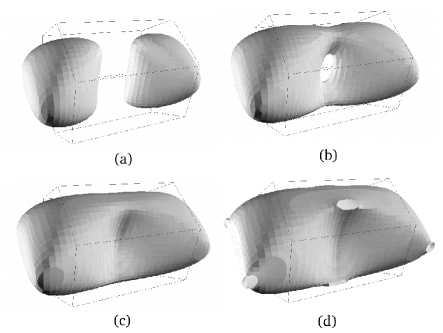
Figure 4: Changes in the topology of the energy surface ($H(Z_{A},Z_{B},\Phi_{B})=E$ with $\Phi_{A}=0$), for $\sigma>2/3,$ here $\sigma=0.75$. (a)$E=-0.92,$ (b) $E=-=0.98$, (c) $E=-1.02$, and (d) $E=-1.1.$ The hexagonal prism represents the hexagonal boundaries of the $(Z_{A},Z_{B})$ plane: the horizontal direction is $Z_{A}$, the vertical direction is $Z_{B}$ and the long axis of the prism is $\Phi_{B}.$ The endpoints of the prism are at $\Phi_{B}={2\sqrt{2}\over 3}\pi$ and $\Phi_{B}={4\sqrt{2}\over 3}\pi.$

Figure 6: The classical density of states as a function of energy for $\sigma=0.6$ determined by numerical integration. (a) the coalescence transition, (b) the lower polar transition, (c) the antiparallel transition. The total area under the curve is $3\pi,$ the volume of the reduced phase space.

Figure 7: Energy-period curve of the three spin system with $\sigma=0.5.$ (a) Stationary Spin, (b) Counterbalanced, (c) Three-phase orbit, and (d) Unbalanced orbits.

Figure 8: The stability exponent $\rho$ ($\rho={\mathrm{Tr}\,}{\mathbf{M}}$ where ${\mathbf{M}}$ is the stability matrix) of the stationary spin orbit as a function of energy for $\sigma=0.5.$ An orbit is stable when $|\rho|<2$ and unstable when $|\rho|>2.$ The stationary spin orbit is stable near the AFM ground state and alternates between being stable and unstable until $E_{c}.$ The outer branch of the orbit is unstable for all $E>E_{c}$ while the inner branch appears to always be stable until its disappearance at $E=1.$

Figure 9: The stability exponent $\rho={\mathrm{Tr}\,}{\mathbf{M}}$ where ${\mathbf{M}}$ is the stability matrix for the counterbalanced orbit in the case $\sigma=0.5$ where the orbit is always stable.

Figure 10: The precession rate squared as a function of energy for the three phase orbit with $\sigma={1\over 2}.$ The precession rate is the amount that $\Phi_{0}$ increases after one period of the orbit in the reduced space. In the limit of $E\rightarrow-{3\over 2}$ the precession rate becomes $2\pi.$ The straight line fit (fit to all of the points with $E>0.90$) indicates $(E-E_{b})^{1\over 2}$ scaling with $E_{b}=-0.7547.$ Note that $(2\pi)^{2}\approx 39.48.$

Figure 11: Stability exponent $\rho$ for the three phase orbits for $\sigma=0.5$. The three phase orbit is stable for $E>E_{b},\ E_{b}\approx 0.75.$ Starting from high energies, $\rho$ reaches $2$ at $E_{b}$ where a bifurcation gives birth to two stable precessing orbits and an unstable nonprecessing orbit. Another (unstudied) bifurcation happens around $E=0.91.$ Starting at the low-energy AFM end, the orbit starts out stable and becomes unstable at $E=-1.32$ in a period doubling bifurcation.

Figure 14: A projection of the $E=-1.39$ Poincaré section into the $(\Phi_{B},Z_{B})$ plane. Orbits marked (a) are three phase orbits, (b) is a stationary spin orbit, and (c) is an unbalanced orbit.

References

- Houle et al. (1999) P. A. Houle, N. G. Zhang, and C. L. Henley, Phys. Rev. B 60, 15179 (1999), eprint cond-mat/9908055.
- Nakamura et al. (1985) K. Nakamura, Y. Nakahara, and A. R. Bishop, Phys. Rev. Lett. 54, 861 (1985).
- Nakamura et al. (1986) K. Nakamura, Y. Okazaki, and A. R. Bishop, Phys. Lett. A 117, 459 (1986).
- Nakamura and Bishop (1986) K. Nakamura and A. R. Bishop, Phys. Rev. B 33, 1963 (1986).
- Nakamura (1993) K. Nakamura, Quantum Chaos: A new paradigm of nonlinear dynamics (Cambridge University Press, 1993).
- Shankar (1980) R. Shankar, Phys. Rev. Lett. 45, 1088 (1980).
- Klein and Li (1981) A. Klein and C. T. Li, Phys. Rev. Lett. 46, 895 (1981).
- Sessoli (1981) R. Sessoli D. Gatteschi, A. Caneschi,and M. A. Novak, Nature 365, 141 (1993).
- Magyari et al. (1987) E. Magyari, H. Thomas, R. Weber, C. Kaufman, and G. Müller, Z. Phys. B 65, 363 (1987).
- Srivastava et al. (1988) N. Srivastava, C. Kaufman, and G. Müller, J. Appl. Phys. 63, 4154 (1988).
- Srivastava et al. (1990) N. Srivastava, C. Kaufman, and G. Müller, J. Appl. Phys. 67, 5627 (1990).
- Srivastava and Müller (1990a) N. Srivastava and G. Müller, Phys. Lett. A 147, 282 (1990a).
- Srivastava and Müller (1990b) N. Srivastava and G. Müller, Z. Phys. B 81, 137 (1990b).
- Srivastava et al. (1991) N. Srivastava, C. Kaufman, and G. Müller, Computers in Physics p. 239 (1991).
- Van Hemmen and Sütö (1986) J. L. Van Hemmen and A. Sütö, Physica B 141, 37 (1986).
- (16) The proportionality depends on the value of for a spin system, or for a particle system. Figure 4 of Houle et al. (1999) compares the classical and quantum densities of state.
- Lichtenberg and Lieberman (1992) A. J. Lichtenberg and M. A. Lieberman, Regular and Chaotic Dynamics (Springer-Verlag, New York, 1992), 2nd ed.
- Gutzwiller (1990) M. C. Gutzwiller, Chaos in Classical and Quantum Dynamics (Springer-Verlag, New York, 1990).
- Gustavson (1966) F. G. Gustavson, The Astronomical Journal 71, 670 (1966).
- Broucke (1985) R. Broucke, Dynamical Astronomy (University of Texas Press, Austin, 1985), pp. 9–20, editors V. Szebehely and B. Blazas.
- Hénon and Heiles (1964) M. Hénon and C. Heiles, Astronomical Journal 69, 73 (1964).
- Houle (1997) P. A. Houle, Phys. Rev. E 56, 3657 (1997), eprint cond-mat/9704118.
- Press et al. (1992) W. H. Press, S. A. Teukolsky, W. T. Vetterling, and B. P. Flannery, Numerical Recipies in C (Cambridge University Press, Cambridge, UK, 1992), 2nd ed., ISBN 0-521-43108-5.
- Hénon (1982) M. Hénon, Physica D 5, 412 (1982).
- Bloomenthal (1988) J. Bloomenthal, Computed Aided Geometric Design 5, 341 (1988).
- Glassner (1990) A. S. Glassner, Graphics Gems (Academic Press, Boston, 1990), ISBN 0-12-286165-5.
- Lorensen and Cline (1987) W. E. Lorensen and H. E. Cline, Computer Graphics 21, 163 (1987).
- Gamma et al. (1995) E. Gamma, R. Helm, R. Johnson, and J. Vlissides, Design Patterns (Addison-Wesley, Reading, MA, 1995), ISBN 0-201-63361-2.
- (29) A category of integrator known as symplectic integrators preserve the symplectic property of classical mechanics McLachlan and Atela (1992) and are claimed to be more qualitatively accurate for very long integration times than conventional integrators. Because we were only interested in short-term time evolution and because there is no systematic procedure for deriving a symplectic integrator for an arbitrary problem, we did not make the investment of developing a symplectic integrator for our system.
- McLachlan and Atela (1992) R. I. McLachlan and P. Atela, Nonlinearity 5, 541 (1992).