Tailoring the profile and interactions of optical localized structures

Abstract

We experimentally demonstrate the broad tunability of the main features of optical localized structures (LS) in a nonlinear interferometer. By discussing how a single LS depends on the system spatial frequency bandwidth, we show that a modification of its tail leads to the possibility of tuning the interactions between LS pairs, and thus the equilibrium distances at which LS bound states form. This is in agreement with a general theoretical model describing weak interactions of LS in nonlinear dissipative systems.

Localization of spatial patterns is a subject of major current interest in the research on nonlinear dissipative dynamical systems. The studies about this topics have naturally followed and sided those dedicated to the formation of temporal and spatial solitons in Hamiltonian systems solitoniHamilton . Analytical and numerical works have identified several distinct mechanisms leading to structure localization in dissipative systems Riecke , and experimental observations of this phenomenon have been recently offered in several systems, such as fluid dynamics solitonifluidi , chemistry solitonichimici , granular materials solitonigranulari and nonlinear optics solitoniottici .

In particular, optical localized structures (LS), to which we will also refer to as dissipative solitons in the following, are objects of intense research, also in view of possible applications as pixels in devices for information storage or processing. So far, the existence of optical dissipative solitons has been theoretically predicted in many passive Tlidi and active sistemiattivi configurations, and optical LS have been observed in photorefractive cavities AndersonWeiss1 and in passive nonlinear interferometers, based either on the ”thin slice with feedback” scheme DarmstadtLS ; MuensterLS ; NoiLS , or on a microresonator filled with a semiconductor medium KuscelewitzTredicce . More recently, the interactions between LS have been shown to give rise to the formation of a discrete set of bound states MuensterLS .

To our knowledge, very little is known about the dependence of the LS’s features on the experimental parameters. The present work addresses this issue, by investigating how the spatial frequency bandwidth of a nonlinear interferometer can be utilized to tune both the spatial profile of each single soliton, and the interaction forces occurring between two of them. A quantitative experimental evidence is given of the crucial role played by the oscillatory tails of a single LS in determining the interaction forces between solitons.

Our experimental system consists of a Liquid Crystal Light Valve (LCLV) closed in an optical feedback containing both interferential and diffractive processes. When an initially plane wave is sent into the system, its phase $\varphi(\vec{r},t)$ evolves according to NoiLS

$$\tau{\partial\varphi\over\partial t}=-(\varphi-\varphi_{0})+l_{d}^{2}\nabla^{2}_{\perp}\varphi+\alpha I_{0}\mid e^{{-il\nabla^{2}}\over{2k_{0}}}(Be^{-i\varphi}+C)\mid^{2}$$ (1)

where $\varphi_{0}=\pi$ is the phase working point of the LCLV, and $\tau$ and $l_{d}$ are its response time and diffusion length respectively. The source term in the right hand side of Eq. (1) depends on the free propagation length $l$ in the feedback loop, as well as on the laser light wavenumber $k_{0}$ and on the parameters $B$ and $C$, that tune the relative weight of diffraction and interference in the system. Finally, $I_{0}$ is the incident laser intensity, and $\alpha$ describes the Kerr-like response of the LCLV. Here, $B=\cos^{2}\theta$, $C=\sin^{2}\theta$, where $\theta$ is the (experimentally adjustable) angle between the director of the nematic liquid crystals of the LCLV and the transmissive axis of a polarizer oriented along the polarization direction of the incident light.

In a previous work NoiLS , we have characterized the state diagram of the interferometer in the parameter plane $(\theta,I_{0})$, finding that localization of patterns occurs for a broad range of $\theta$ values ($\simeq 35^{o}$ to $58^{o}$). This phenomenon is related to the presence of a subcritical bifurcation, connecting a lower uniform branch to an upper patterned one. In these conditions, the formation of isolated spots connecting the two branches is typical Tlidi ; sistemipassivi ; Aranson . Besides $\theta$ and $I_{0}$, the scenario of observable patterns crucially depends on the spatial frequency bandwidth $q_{B}$ of the interferometer, which can be experimentally controlled by means of a variable aperture put in a Fourier plane. In what follows we discuss the main LS features that emerge by keeping fixed $\theta=42^{o}$, and varying $I_{0}$ and the adimensional parameter $q_{b}\equiv{q_{B}}/{q_{\text{diff}}}$ obtained by normalizing the system bandwidth to the diffractive interferometer wavenumber $q_{\text{diff}}=\sqrt{\frac{\pi k_{0}}{l}}$.

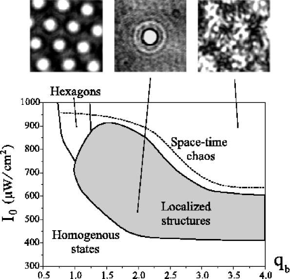
Figure 1: State diagram of the system in the ($q_{b},I_{0}$) parameter plane. Notice that LS emerge for a broad range of parameters (gray area in the plane). The three reported patterns are snapshots of the observed hexagons, LS, and space time chaotic states.

A first point of interest is to establish the range of existence of LS in the ($q_{b},I_{0}$) plane. In Fig. 1 we plot the state diagram of the system in this parameter plane, together with some snapshots representative of the observed patterns. All the experiments are performed at incident laser wavelength $\lambda=632$ nm and for $l=250$ mm. This results in a scale of the observed patterns of the order of $2\pi/q_{\text{diff}}\simeq 0.5$ mm.

Looking at Fig.1, one easily realizes that the range of existence of LS is very broad, not at all limited to some particular parameter choices. The lower threshold for the existence of LS increases for decreasing $q_{b}$. This is a consequence of the fact that LS have an internal structure conatining both low and high frequency components, as it will appear evident in the following. Therefore, any bandwidth limitation perturbs the LS structure, and increases the threshold for their existence. At very low $q_{b}$ and high intensities, localization of structures is lost and regular hexagons are observed, due to the long range correlation imposed to the pattern by the small bandwidth.

If $I_{0}$ is kept fixed at high values while $q_{b}$ is increased, hexagonal patterns evolve into a space-time chaotic (STC) regime. The boundary line between STC and LS occurs at decreasing intensities when $q_{b}$ is increased. This indicates that the regime here generically referred to as STC can arise either from a strong excitation of a relatively small band of wavenumbers, or from a weak excitation of a large set of interacting spatial modes. The indetermination of the boundaries between the different regimes is of the order of 10 %. It must be also specified that the placement of the boundaries depends on the evolutionary history of the parameters, since we are in presence of a subcritical bifurcation. The continuous lines in Fig. 1 were obtained by decreasing the input intensity, the dashed line by increasing it. Localized structures are not observed in this last case.

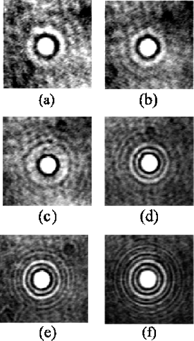
Figure 2: Variation of the LS’s shape with the system bandwidth. Snapshots of the observed solitons for (a) $q_{b}=1.0,I_{0}=700\ \mu W/cm^{2}$ (b) $q_{b}=1.2,I_{0}=620\ \mu W/cm^{2}$, (c) $q_{b}=1.6,I_{0}=520\ \mu W/cm^{2}$, (d) $q_{b}=2.2,I_{0}=480\ \mu W/cm^{2}$, (e) $q_{b}=2.8,I_{0}=460\ \mu W/cm^{2}$, (f) $q_{b}=4.0,I_{0}=460\ \mu W/cm^{2}$.

Scanning the parameters within the domain of LS’s existence leads to sensible modifications in the shape of each structure. In Fig. 2 we show the variation in the LS intensity profile observed by keeping $I_{0}$ close to the lower threshold for LS existence and increasing $q_{b}$. It is seen here that each structure is formed by a central peak, and by a set of concentric rings forming a tail that shows spatial oscillations of decreasing amplitudes for increasing distances from the LS center. The width of the central peak can be roughly evaluated as the diameter of the first dark ring in each frame, and appears to be practically independent on $q_{b}$.

The length scale of the oscillations on the tails is instead strongly dependent on $q_{b}$. Namely, this scale decreases for increasing $q_{b}$ until $q_{b}\simeq 3$, and then saturates to a constant value.

The set of our observations indicates that LS have a ”natural” unperturbed shape like that displayed for $q_{b}\geq 3$. By constraining the system to a bandwidth smaller than this value, one is then able to tune the LS profile, imposing oscillations on the tails at a frequency different from the natural one. The occurrence of oscillatory tails on LS have been reported in other physical systems Aranson ; tails1 , and it is considered to be a typical signature of the formation of LS via pinning of the fronts connecting the uniform and the patterned states Riecke .

The observed LS closely resemble those reported in Ref. Aranson , in which a subcritical real Swift-Hohenberg (S-H) equation is studied analytically and numerically. This is not surprising, since our experiment displays a subcritical bifurcation of a real order parameter to a patterned state, and therefore is appropriately modeled by an order parameter equation of that kind. We do not expect that the S-H model describes faithfully all the details observed in the experiiment, however. It is known Neubecker , for example, that the ”thin slice with feedback” model, of which our experiment is an implementation, presents instabilities at multiple wavenumbers given by $q_{\text{N}}=\sqrt{N}q_{\text{diff}}$, $N=1,5,9,...$. Though the highest wavenumbers become active at high values of pump parameter due to diffusion, it may be expected that they play some role in determining the fine features of the LS’s. Our aim in comparing the experimental findings wit the prediction of the S-H model is indeed to investigate wheter some fundamental features of the observed phenomena can be described in terms of this very general model.

Using the Swift-Hohenberg model, it is found analytically that the LS tails are described by single spatial scale oscillations, embedded in an exponential envelope that departs from the lower uniform state.

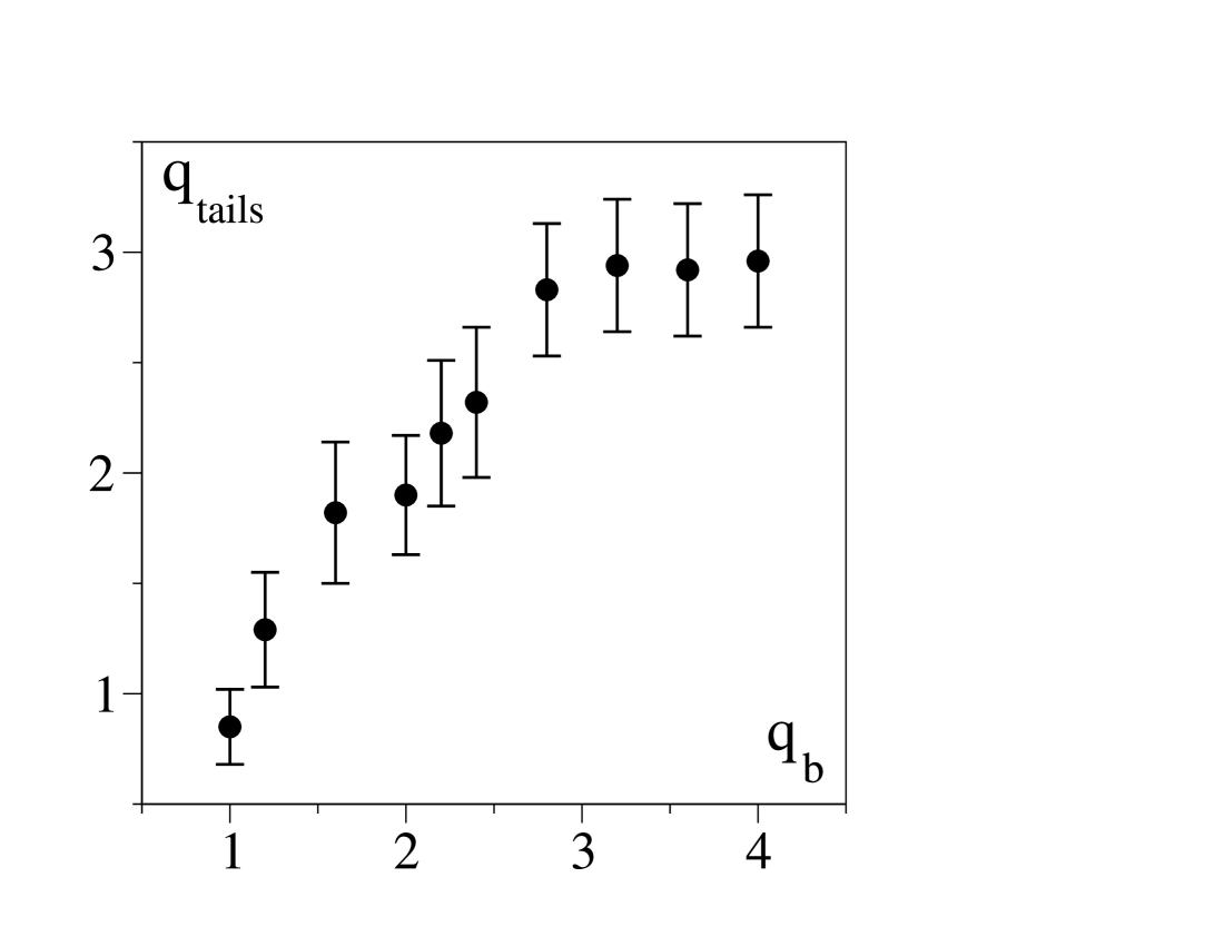
Figure 3: Variation in the main frequency of the LS tail oscillations as a function of the system bandwidth. Both $q_{\text{tails}}$ and $q_{b}$ are adimensional quantities (see text for definition).

Though the LS tails in our case display some deviations from the above ideal behavior, the qualitative agreement between our observations and the results of the general theory reported in Ref. Aranson is satisfactory. In particular, it is possible to identify for each value of $q_{b}$ a dominating spatial scale in the oscillatory tails. To this purpose, we measure the distance between successive maxima of a single LS and average this quantity over all observed maxima. This way, we obtain the dominant spatial frequency of the tail oscillations, which is then normalized to $q_{\text{diff}}$ and reported as $q_{\text{tails}}$ in Fig. 3. The error bars correspond to the measured frequency fluctuations from the $q_{\text{tails}}$, reflecting the fact that the tail oscillations are not rigorously at a single spatial scale. Looking at Fig. 3, one easily realizes that $q_{\text{tails}}$ practically coincides with $q_{b}$ for $q_{b}\leq 3$. At higher values of $q_{b}$, no variations in $q_{\text{tails}}$ as well as in overall LS’s profile are observed.

The shape of the tails is responsible for the interactions between localized structures. Namely, while for monotonically decreasing tails, one would expect only attractive or repulsive forces between LS, oscillatory tails induce oscillatory signs of the interactions, thus producing both attractive and repulsive forces, depending on the distance between the centers of a pair of LS’s Aranson ; tails1 . A recent work MuensterLS has experimentally demonstrated the existence of a discrete set of LS bound states, occurring in the presence of oscillations on the LS tails. The selection rule for the discrete set of bound states observed has been there put in relation with the spacing of their rings originated by diffraction around the central peak. In the following we show how these bound states can be in fact tuned by varying the spatial frequency bandwidth of the interferometer, and we discuss how the selection of the observed bound ststes can be put in the very general framework of a subcritical S-H model.

In Fig. 4 we display a set of different bound states observed for $q_{b}$ = 3.6. We notice that the states form a set that can be ordered following a precise rule, given by simply counting of the number of maxima and minima that occur along the segment connecting the two LS centers. We will call this number $n$ as bound state order number. Such a feature is encountered for all values of $q_{b}$. At small system bandwidths, however, we observe only the first two or three bound states, instead of the entire set shown in Fig. 4. This is probably due to the fact that the binding energy of each state varies with $q_{b}$, and in some cases it is not sufficient to keep the LS pair tightly bound in the presence of unavoidable system inhomogeneities and fluctuations.

A theory for the interaction of LS pairs was given in Ref. Aranson in the context of study on a real Swift-Hohenberg equation. As already discussed, we expect this model to be closely applicable to our system in the present conditions. Following that approach, the weak interactions between a pair of LS with tails decaying with a length $\mu$ and oscillating at a frequency $\nu$, lead to a time evolution for the distance $R$ between the LS centers ruled by

$${dR\over dt}={1\over R}{d\over dR}(e^{-\mu R}cos(\nu R))\equiv F(R,\mu,\nu).$$ (2)

As a consequence, an infinite number of stable bound states are possible, corresponding to the solutions $F=0$, $dF/dR<0$ of Eq. (2). In the limit in which the scales $\mu$ and $\nu$ are well separated, the difference $R_{n+1}-R_{n}$ between the separation distances of two successive bound states corresponds approximately to the tail oscillation length ${\nu}^{-1}$ of a single LS. We recall that by weak interaction we mean a regime in which the intensity amplitude of one LS is small in the space region in which the intensity amplitude of the other is large. In the case of our experimental data, this is true for all the bound states observed, with the possible exception of the lowest order one.

If we assume that Eq. (2) describes correctly the bound state selection rule in our experiment, it immediately follows that tuning of the equilibrium distances should be possible by varying the scale of the oscillations on the tails of each single LS. In order to check this point, we measured the quantities $\Delta_{n,n+1}=R_{n+1}-R_{n}$, and then averaged them over the bound state order number $n$. The resulting quantity $\bar{d}$ (normalized to the length $\Lambda_{\text{tails}}$) is reported vs. $q_{b}$ in Fig. 5. A constant value of the ratio ${{\bar{d}}\over\Lambda_{\text{tails}}}\simeq 1$ is observed within the errors, indicating that the above discussed relation between the oscillations on the tails of each LS and the selection rule of bound states is verified. This marks the fact that tuning of the equilibrium distances between LS’s in bound states can be quantitatively performed in our experiment.

In conclusion, we have given a quantitative evidence of the tuning of the LS spatial profile in a nonlinear optical interferometer, using the system spatial frequency bandwidth as a control parameter. We have discussed the role of the oscillations occurring on each single LS tail in determining the interactions between different LS’s. Finally, we have verified the agreement between the selection rules for the formation of bound states observed in our experiment, and those predicted for the same phenomenon by a general model for pattern formation in nonequilibrium systems.

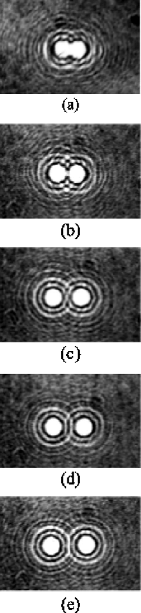
Figure 4: Snapshots of different bound states observed at $q_{b}=3.6,I_{0}=500\ \mu W/cm^{2}$. All patterns (a-e) are obtained by inducing a pair of LS with an increasing initial distance between centers, and letting the system evolve up to the time at which the stationary bound state is realized.

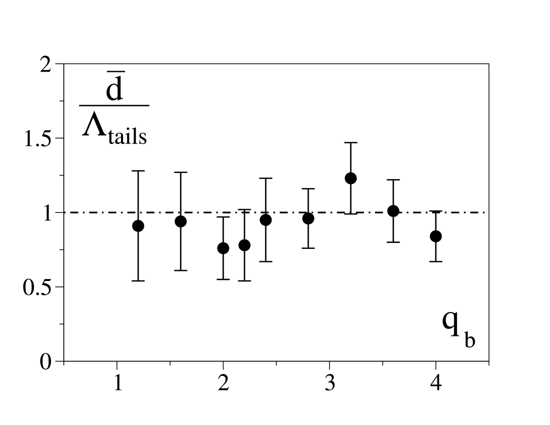
Figure 5: ${{\bar{d}}\over\Lambda_{\text{tails}}}$ vs. $q_{b}$ (see text for definitions). Both quantities are adimensional. Notice that, for all measurement a constant value of ${{\bar{d}}\over\Lambda_{\text{tails}}}\sim 1$ is realized within the experimental errors.

References

- (1) See e.g. E. Infeld and G. Rowlands, Nonlinear waves, solitons and chaos, (2nd ed., Cambridge University Press, 2000).
- (2) H. Riecke, ”Localized structures in Pattern-Forming Systems” in Pattern Formation in Continuous and Coupled Systems, ed. by M. Golubitsky, D. Luss and S. Strogatz (IMA Volume 115, Springer, 1999), p. 215.
- (3) E. Moses, J. Fineberg and V. Steinberg, Phys. Rev. A35, 2757 (1987).
- (4) H. H. Rotermund, S. Jakubith, A. Von Oertzen and G. Ertl, Phys. Rev. Lett. 66, 3083 (1991).
- (5) P. Umbanhowar, F. Melo and H. Swinney, Nature 382, 793 (1996).
- (6) F.T. Arecchi, S. Boccaletti and P.L. Ramazza, Phys. Rep. 318, 1 (1999).
- (7) M. Tlidi, P. Mandel and R. Lefever, Phys. Rev. Lett. 73, 1328 (1994).
- (8) N.N. Rosanov, A. V. Fedorov, S.V. Fedorov and G.V. Khitrova, JETP 80, 199 (1995).
- (9) M. Saffman, D. Montgomery and D.Z. Anderson, Opt. Lett. 19, 518 (1994); V. B. Taranenko, K. Staliunas and C.O. Weiss, Phys. Rev. Lett. 81, 2236 (1998).
- (10) A. Schreiber, B. Thuring, M. Kreuzer and T. Tschudi, Opt. Comm. 136, 415 (1997).
- (11) B. Schapers, M. Feldmann, T. Ackemann and W. Lange, Phys. Rev. Lett. 85, 748 (2000).
- (12) P.L. Ramazza, S. Ducci, S. Boccaletti and F.T. Arecchi, J. of Optics B: Quantum and Semiclassical Optics 2, 399 (2000).
- (13) V.B. Taranenko, I. Ganne, R.J. Kuszelewicz and C.O. Weiss, Phys. Rev. A61, 063818 (2000); J. Tredicce, Communication at the sixth Experimental Chaos Conference, Potsdam, Germany (2001).
- (14) W. J. Firth and A.J. Scroggie, Phys. Rev. Lett. 76, 1623 (1996); L. Spinelli, G. Tissoni, M. Brambilla, F. Prati and L. A. Lugiato, Phys. Rev. A58, 2542 (1998).
- (15) I.S. Aranson, K.A. Gorshkov, A.S. Lomov and M.I. Rabinovich, Physica D43, 435 (1990).
- (16) R. Neubecker, G.L. Oppo, B. Thuering and T. Tschudi, Phys. Rev. A52, 791 (1995).
- (17) C. Schenk, P. Schultz, M. Bode and H.G. Purwins, Phys. Rev. E57, 6480 (1998).