Detecting Determinism in High Dimensional Chaotic Systems

Abstract

A method based upon the statistical evaluation of the differentiability of the measure along the trajectory is used to identify determinism in high dimensional systems. The results show that the method is suitable for discriminating stochastic from deterministic systems even if the dimension of the latter is as high as 13. The method is shown to succeed in identifying determinism in electro–encephalogram signals simulated by means of a high dimensional system.

I Introduction

Although numerous methods have been developed in recent years addressed to detect determinism in time series [1, 2, 3, 4, 5], most of them give wrong or ambiguous results when applied to high dimensional systems (we refer to systems with attractor’s dimension greater than, say, five). However, high dimensional systems are ubiquitous in nature, as for example in the case of spatially extended systems. Therefore it remains the task to develop a robust method capable of detecting deterministic behavior in systems with many active degrees of freedom [6].

We hereby claim that, contrary to some widely accepted premises in the chaos community [7, 8, 9], it is possible to discriminate determinism from stochasticity in systems with a high correlation (or information) dimension. Our method is based upon a fundamental property of deterministic systems, namely, the differentiability of the measure along the trajectory. Our numerical implementation of this property is robust enough to uncover this topological property in short data sets.

As a very first step, we should clarify what we mean by determinism. Attaching to definitions, saying that a time series stems from a deterministic system only if it can be produced by a discrete- or continuous-time dynamics without any stochastic source, would isolate a very small class of phenomena. In fact, even artificial time series from non-stochastic dynamical systems are typically affected by numerical noise, which at best can be considered to be in its zero-limit. Unfortunately, numerical errors tend to be magnified with the reconstruction process and can mimic the effect of a stochastic feedback. It is pertinent to note that Casdagli et al. [10] have shown that univariate time series derived from sufficiently high dimensional systems cannot in practice be regarded as noise-free.

On the other hand, the importance of detecting a possible deterministic dynamics is not merely academic and it is often motivated by the intention of controlling the non-stochastic part of the system under investigation. Thus, operationally, we prefer to imagine an underlying dynamics composed by a stochastic part (that is, dynamical noise) and a non-stochastic one. In this sense, it’s not always obvious how to measure the weight of one part with respect to the other. However, it seems very natural to classify as purely stochastic a system which has not residual (non-trivial) dynamics if its stochastic part is switched off. For example, this is the case of Eqs. (7) and (8) that will be discussed later on. More generally, we speak of determinism whenever the dynamics has a relevant non-stochastic backbone, being conscious that we can decide if this is really non-negligible only when we adopt a suitable indicator. In this paper we make use of the statistical differentiability of the measure as introduced in refs. [11, 12]. There it is argued that this quantity is sensible to the amount of dynamical noise intrinsic to the system. Here we explore the two opposite sides of the scenario depicted above, showing that it sharply discriminates purely stochastic systems from deterministic dynamics, even when the latter takes place on rather high dimensional attractors.

II Methods

A Tracking the measure along the trajectory

To illustrate the point, let’s consider a dissipative dynamical system described by $n$-first-order differential equations ${\bf{\dot{x}}}={\bf F}({\bf x})$. The corresponding flow ${\it f}^{t}$ maps a ”typical” initial condition ${\bf x}_{0}$ into ${\bf x}(t)={\it f}^{t}({\bf x}_{0})$ at time $t$. Once transients are over, the motion settles over the attractor ${\cal A}$. Defined over this set is the natural measure, which, from an operational point of view, can be considered as the limiting distribution of almost all starting initial conditions, that is,

$$\mu(B_{r}({\bf x}))=\lim_{t\rightarrow\infty}{1\over t}\int_{0}^{t}1_{B_{r}}(f^{\tau}({\bf y}_{0}))\>{\rm d}\tau$$ (1)

for almost all ${\bf y}_{0}$ in the basin of attraction. In Eq. (1) $B_{r}(\bf{x})$ indicates the hyper-sphere of radius $r$ centered at $\bf{x}$ and $1_{B_{r}}$ the associated characteristic function. In principle, with infinitely many data points and aribrarily fine sampling, one would consider the limit $r\rightarrow 0$. In practice a suitable density estimator is needed. Here we adopt a fixed-volume Epanechnikov kernel [11, 12], with a compact support $B_{r}$ and a given finite radius $r$ (see below). As shown previously [11, 12], smoothness of this measure along the trajectory is a good candidate to quantify determinism. Numerically, the differentiability of the measure along the trajectory was evaluated by means of the topological statistics developed by Pecora et al. [13]. Actually we look at the continuity of the logarithmic derivative of the measure (see [12]).

We want to emphasize that in looking at this property of the measure we avoid one of the most common problems found in this kind of algorithms, namely, the lack of an acceptable scaling region. In fact, this is the main problem encountered when dealing with quantities such as the maximal Lyapunov exponents and/or Kolmogorov entropy [8], particularly in the case of high dimensional systems (see ref. [6]). Especially troublesome is the calculation of the information ($D_{1}$) or correlation ($D_{2}$) dimensions, in which the search for a reliable scaling region is the source of most of the misuse of the algorithm. Contrarily, our algorithm needs a realible estimation of the natural measure on the attractor not in a range of scales but at a fixed one. There is a lower value of resolution given by the minimun average interpoint distance, which can be estimated as $r_{min}\sim N^{-2/D_{2}}$, and an upper limit given by the attractor extent (which we always normalize to the unit hyper-square) [14]. Below the lower limit there would be statistical fluctuations due to the lack of neighboring points, while close to the upper limit we must confront edge effects [14, 15]. The latter are particularly important for high embedding dimensions because, as the dimension increases, more points stay near the attractor boundary. These bounds are by no means exact, for instance the expression for the lower limit was derived by assuming the data points to be uniformly distributed over the attractor, which is not always true even in cases as simple as nonlinear oscillators. In practice one should look in each particular case for the most appropriate scale to fix. As far as the systems discussed here are concerned, we have found that setting $r$ at 10% of the attractors’ linear extent is a good choice.

B Statistical tests of continuity

A naive test to quantify noise in signals is to check how smooth they are. As long as more noise contaminates the signal, more discontinuous it becomes. This is the case for example of additive noise, e.g. noise added to the signal [6, 16]. However, this is by no means a general rule. For instance, dynamical noise, that is, noise added in the equation of motion, is not expected to affect the smoothness of the signal. We overcome this drawback by using the distribution of points on the trajectory (or the natural measure) as a way to evaluate the degree of noise in the system (see [12]). In order to test the mathematical properties of the measure, that is, continuity, differentiability, inverse differentiability and injectivity, we borrow the statistical approach developed by Pecora et al. [13]. Basically, the method is intended to evaluate, in terms of probability or confidence levels, whether two data sets are related by a mapping having the continuity property: A function $f$ is said to be continuous at a point ${\bf x}_{0}$ if $\forall\epsilon>0,\exists\delta>0$ such that $\parallel{\bf x}-{\bf x}_{0}\parallel<\delta\Rightarrow\parallel f({\bf x}))-f({\bf x}_{0})\parallel<\epsilon$. The results are tested against the null–hypothesis, specifically, the case in which no functional relation between points along the trajectory and the measure exists. Thus, as done in [13], we calculate

$$\Theta_{C^{0}}(\epsilon)=\frac{1}{n_{p}}\sum_{j=1}^{n_{p}}\Theta_{C^{0}}(\epsilon,j)$$ (2)

and

$$\Theta_{C^{0}}(\epsilon,j)=1-\frac{p_{j}}{P_{\rm max}}$$ (3)

where $p_{j}$ is the probability that all of the points in the $\delta$-set, around a given point ${\bf x}_{j}$, of the reconstructed trajectory, fall in the $\epsilon$-set around $\frac{d{\ln\mu({\bf x}_{j})}}{dt}$. The likelihood that this will happen must be relative to the most likely event under the null hypothesis, $P_{\rm max}$ (see refs. [13] and [16]). When $\Theta_{C^{0}}(\epsilon,j)\approx 1$ we can confidently reject the null hypothesis, and assume that there exists a continuous function. As in the work of Pecora et al. [13] the $\epsilon$ scale is relative to the standard deviation of the density time series, and thus, $\epsilon\in[0,1]$. Plots of $\Theta_{C^{0}}(\epsilon)$ versus $\epsilon$ can be used to quantify the degree of statistical continuity of a given function. The typical outcome is a sigmoidal curve whose width and slope are affected by the level and the type of noise contained in the series [11, 12, 16]. In order to characterize the continuity statistics by means of a single parameter we can also calculate,

$$\theta=\int_{0}^{1}\Theta_{C^{0}}(\epsilon){\rm d}\epsilon$$ (4)

The limiting values of $\theta$, namely, 0 and 1, correspond to a strongly discontinuous and a fully continuous function, respectively. Hereafter we shall refer to $\theta$ as CS (Continuity Statistics).

III Results

A Generalized Mackey-Glass system

In order to investigate how our algorithm work on high dimensional systems, we use a generalization of the Mackey-Glass (MG) equation [17], a delayed feedback system,

$${\dot{x}(t)} = \frac{ax(t-\tau_{0})}{1+x^{10}(t-\tau_{0})}-y(t)$$ (5)

$${\dot{y}(t)} = -\omega^{2}x(t)-\rho y(t)$$ (6)

where $a=3$, $\rho=1.5$, $\omega=1$ and $\tau_{0}=10$. As it is stated in ref. [17] the Kaplan-Yorke dimension of this system is $D_{KY}\sim 13.5$, which, according to the Kaplan-Yorke conjecture, $D_{KY}=D_{1}$, for a typical attractor. We have made a standard reconstruction analysis over time series of up to 16384 data points. Although the optimal time delay $\tau$ should be given by the first minimum of the mutual information, $210$ in sampling units, we have used a somewhat smaller value, typically $120$. Using larger delays in high embedding dimensions would reduce drastically the number of reconstructed points. The choice of this value, however, is supported by the fact that in high dimensions, the optimal $\tau$ seems to be smaller than that given by the mutual information criterion [18], at least in the case of chaotic continuous-time systems, as our case. Surrogate time series [19, 20] with the same number of points have also been generated, using the routines in the TISEAN [21] package (“endtoend” and “surrogates”).

We have also calculated the correlation integral of this system. As it is well known, this is the most basic procedure to discriminate between deterministic and stochastic behavior. The numerical results for the correlation integral and its derivative (that gives the correlation dimension) are shown in Figure 1. The results show that, for this high dimensional system, no region with constant slope is found. This clearly illustrates the well known difficulties inherent to the estimation of the correlation dimension in high dimensional systems.

In Figure 2 we report the values of CS for the generalized MG system (reconstruction from the $x$-time series) when the embedding dimension is varied in the range 2–30. In order to increase the robustness of the results, we have averaged the CS for six differents time series. The high values corresponding to the original series, together with the lower values of their surrogates, indicate that our method is able to identify determinism in a high dimensional system. We also note that whereas the CS for the original series remains almost constant for embedding dimensions larger than the correlation dimension, that for the surrogate series decreases steadily. Finally, it is here pertinent to observe that the results of ref. [12] are referred to the standard MG equation (see Eq. (27) in the Appendix), whose correlation dimension is estimated around seven [2], while here we have choosed the generalization (6) just to check that the methodology works with more severe test. However, despite the smaller correlation dimension, in Fig. 8 of [12] the CS for the standard MG system is lower than the CS for the generalized version reported here. In the Appendix we discuss the solution to this apparent paradox, through a digression on the role of the sampling time on the observed levels of CS.

B Simple stochastic systems

As already remarked above, the results just discussed have to be contrasted with those obtained for stochastic systems. Here we show results for two time series derived from a linear (7) and a nonlinear (8) stochastic processes, namely,

$${\dot{x}} = \theta x(t)+\eta(t)$$ (7)

$${\dot{y}} = (\alpha-0.5)\beta-y(t)+\sqrt{2\beta y(t)}\eta(t)$$ (8)

where $\eta(t)$ is a Gaussian noise with standard deviation 0.1, $\alpha=\beta=1$, and $\theta=-0.9$. Both processes are examples of purely stochastic systems, as no dynamics is left in the noise free limit, and exhibit $(1/f^{\alpha})$ power law spectra, a finite correlation dimension ($\approx 2$) and a converging Kolmogorov entropy [22]. Note that this is a typical case in which the correlation dimension fails in identifying stochasticity.

Attractor reconstruction was carried out on time series with up to 8192 data points and a time delay of 100 (somewhat less than the first minimum of the mutual information which in this case lies approximately at 130). As it is clearly seen in Figure 3, there is no difference between the CS for the orginal time series and its surrogate, both showing very low values which indicate a low differentiability (a signature of stochasticity as discussed in [12]).

C Model of Electro-encephalogram signals

A paradigmatic example of high dimensional systems is found in physiology, namely, Electro-encephalogram (EEG) signals. These are in fact the result of a sum over a large number of neuronal potentials. There are many studies that claim deterministic behavior in EEG dynamics, most of them based on the calculation of the correlation dimension. However, recent analyses have pointed out many technical problems related to those studies (see [9] and references therein) which throw serious doubts on the above conclusion. We have applied our method to the analysis of a EEG-like signal [9] generated by the following set of nonlinear coupled equations,

$${\dot{x}_{1}}=x_{2}$$ (10)

$${\dot{x}_{2}}=\frac{x_{5}-25}{3}{\rm sin}\omega_{1}t+3x_{7}{\rm sin}\omega_{2}t$$ (11)

$$+x_{11}{\rm sin}\omega_{2}t-3|x_{6}|x_{2}-x_{9}x_{1}$$ (12)

with $\omega_{1}$=30, $\omega_{2}$=65 and $\omega_{3}$=80;

$${\dot{x}_{3}}=\sigma(x_{4}-x_{3})$$ (14)

$${\dot{x}_{4}}=-x_{3}x_{5}+rx_{3}-x_{4}$$ (15)

$${\dot{x}_{5}}=x_{3}x_{4}-bx_{5}$$ (16)

where $\sigma$=10, $r$=28 and $b$=8/3 (Lorenz system).

$${\dot{x}_{6}}=x_{7}$$ (18)

$${\dot{x}_{7}}=-kx_{7}-x_{6}^{3}+B{\rm cos}t$$ (19)

where $k$=0.1 and $B$=12 (Ueda equations).

$${\dot{x}_{8}}=x_{9}$$ (21)

$${\dot{x}_{9}}=-\delta x_{9}+\frac{1}{2}x_{8}(1-x_{8}^{2})+f{\rm cos}\omega t$$ (22)

where $\delta$=0.15, $F$=0.15 and $\omega$=0.8 (two–well potential Duffing–Holmes attractor).

$${\dot{x}_{10}}=-(x_{11}+x_{12})$$ (24)

$${\dot{x}_{11}}=x_{10}+\alpha_{11}$$ (25)

$${\dot{x}_{12}}=\alpha+x_{12}(x_{10}-\mu)$$ (26)

where $\alpha$=0.15 and $\mu$=10 (Rössler attractor). This intricate system has a correlation dimension around 9 and has failed to pass the method originally proposed by Salvino and Cawley [4].

We have integrated the whole system of [9] using a fourth-order Runge-Kutta algorithm with a fixed step of 0.001. The main two coordinates, $x_{1}$ and $x_{2}$, behave in a markedly different way. Coordinate $x_{2}$ shows a rather standard behavior with the first zero of the autocorrelation function lying at $\simeq 27$ (in units of sampling time). Instead, the $x_{1}$ time series exhibits a power spectrum that seems to be of the $1/f^{2}$ type and a first zero of the autocorrelation that strongly depends on the series length $N$. We found $1.3\times 10^{4}$ for $N=10^{5}$ and $9.9\times 10^{4}$ for $N=10^{6}$ (both in units of a larger time step, namely 0.01, that was used to analyze longer time series). These results may reveal a non-stationary behavior of $x_{1}$. In fact this coordinate shows a saw-tooth shape with a very long wavelength and, as a consequence, it may appear to increase linearly over rather long time intervals. As the analysis of [9] was done on the $x_{1}$ coordinate it may actually be the reason why those authors failed in detecting determinism in this system. Note that the lack of stationarity (a property related to ergodicity) would imply the failure of our method. A proper estimation of the (reconstructed) measure, requires that space averages correspond to time averages, which in fact would be impossible if the time series is not stationary. This is the reason why we cannot estimate confidently the measure along the trajectory using $x_{1}$ in the above system. However, as ${\dot{x}_{1}}=x_{2}$, this allow us a better estimate from the $x_{2}$ coordinate (since upon differentiating [1] the saw–tooth shape of the $x_{1}$-time series coordinate results in very small offsets).

Figure 4 shows the CS for both the $x_{2}$ time series and its surrogate. We have averaged over 8 differents realizations and their corresponding surrogates. The results correspond to time series having 4096 data points and a time delay of 27 (in this case the first zero of the autocorrelation function and the first minimum of the mutual information almost coincide). The difference between the CS for the original series and that for its surrogate is noticeable, even on such short time series. This, along with the high value of CS obtained for the original series [12], reveals an essentially deterministic origin of the simulated EEG signal.

IV Discussion

The examples discussed in the previous section indicate that the analysis of the CS with respect to the embedding dimension reveals useful informations in order to discriminate stochasticity from determinism. Despite the high dimensionality of the deterministic systems we notice that the distinction is feasible almost from the start, that is, from dimensions lower than the attractor dimension. This is an interesting (though somehow “fortunate”) outcome since, for such low embedding dimensions, transverse self-intersections of the orbit must occur (or equivalently the existence of false nearest neighbors). However, as the embedding dimension increases, and especially beyond the correlation dimension of the system, the CS of the original signal seems to stabilize around a constant value. Contrarily, the CS for the surrogated series steadily decreases for embedding dimensions larger than the correlation dimension (compare Figures 2 and 4). Finally, the CS for the purely stochastic processes (Figure 3) attains rather low values and is monotonically decreasing.

The small error bars in the CS, both in Figure 2 and 4, indicate that the smoothness of the measure in deterministic systems shows almost no dependence on initial conditions. The absolute value of the CS for deterministic signals may slightly depend on several factors, namely, number of data points, sampling rate, ball size in the measure estimation process, etc. But, for most deterministic time series belonging to different trajectories, the computed CS seems to be a robust measure of the property we want to identify. On the other hand, the CS calculated for the reconstructed measure in the case of the surrogate time series shows a large variability. In noting this we are not only referring to the large error bars of Figures 2 and 4 characteristic of most noisy magnitudes, but rather to the largely different CS found for the systems of those two Figures. In particular we note that, while the CS for the original series are similar and higher than 0.9, those for the surrogated series are, higher than 0.6 in the case of the generalized Mackey-Glass (Fig. 2) and smaller than 0.2 for the EEG signal (Fig. 4). Surrogate time series generated by the IAAFT method [20], as those used here, are in fact, realizations of a Gaussian linear stochastic process (possibly passed through a nonlinear invertible measurement function). By definition, they share the same correlation structure of the original time series and the same probability density function (histogram). In passing, notice that in refs. [11, 12] the results correspond to the simpler AAFT method. Although correlation structure is in some way related to continuity, both are very different properties of the signal. A strict application of the surrogate methodology in our case would requiere to generate surrogates time series with the same continuity characteristics of the original signal. Moreover, and going back to the issue of the absolute value of the CS, we should keep in mind that the statistics of Pecora, Carroll and Heagy [13] are in turn a measure of a certain null-hypotesis. Strictly speaking we are dealing with the superposition of two null-hypotesis and this drawback doesn’t allow a clear interpretation of the CS values coming from surrogate data. It is likely that a different surrogation method is required for a safe application of our method to the analysis of surrogate series derived from nonlinear systems. We are actually investigating this issue in the light of constrained randomization [23].

V Concluding Remarks

Summarizing, we have shown numerically that it is possible to discriminate determinism from stochasticity in high dimensional systems. A local property of the system, as the differentiablity of the measure along the trajectory, prevents us from regarding as ”random” those systems that actually are deterministic (a task in which other methods have failed). The fact that for sufficiently fine sampling and large embedding dimensions the parameter CS for deterministic systems is always above 0.9, opens the possibility of applying our methods to the analysis of more complicated series such as the experimental ones without resorting to comparison with the CS for surrogate series. A lot of work still remains to establish the method as a truly practical tool. For instance, its limits of applicability have to be identified, particularly regarding the relation between the minimum number of data points in the series and the actual dimension of the system. Real applications would require to extract information about the existence of many more (hundred, thousand, etc.) active degrees of freedom of the underlying system. Fortunately, as the results here discussed seem to indicate, this does not necessarily require large embedding dimensions.

VI Appendix: How results depend on sampling

One of the very preliminar steps in time series analysis in to ensure that one is dealing with a good sampling time. The precise meaning of this statement depends somehow on the specific problem at hand. Nonetheless, what is normally done is to check that the sampling time is much smaller than the smallest time scale, $t_{\rm min}$, present in the system. This could be a (quasi) period, an autocorrelation time, an inverse of the maximum Lyapunov exponent and so on. However, there are practical limitations to this rule. Experimentally, the resolution time is not always freely adjustable. Numerically, one should cope with the limited performances of the machine. In both cases, one has to consider also the problem of storing large amount of data. This is fundamental when one realizes that the system possesses intrinsic long time scales, which have to be covered in order to analyze stationary time series. The compromise between series length and stationarity is often achieved by making a re-sampling of the series itself. However, this decimation procedure is not always innocuous. This Appendix is devoted to study how our basic index, the CS, is affected when one takes different sampling time. We take the following three examples. First, time series built from the $x$-coordinate of the Lorenz system ($x_{3}$ in Eqs. (16)). Second, the Mackey-Glass delayed differential equation:

$$\dot{x}=\frac{ax(t-\tau_{0})}{1+x^{10}(t-\tau_{0})}-bx(t)\;,$$ (27)

choosing $a=0.2$, $b=0.1$ and $\tau_{0}=100$. Third, the purely (nonlinear) stochastic system of Eq. (8). In Fig. 5 we report the corresponding CS’s versus the embedding dimension, for various values of the decimation time. The resulting series lengths are 10000 for the Lorenz and MG systems and 20000 for the stochastic process. In every case, the delay time of the reconstruction was choosen as the minimum of the corresponding mutual information. As far as the Lorenz and MG systems are concerned, one sees what it is somehow expected for a discretized continuous function, that is, the coarser is the sampling the lower is the continuity level. Hence, when applying this kind of methods, one should keep in mind that to some extent the CS may be lowered due to a not-so-good sampling. In particular from Figs. 2 and 5 one sees that is in fact the origin of the discrepance, anticipated in Subsection III A, between the MG data shown here and those of ref. [12]. Nevertheless, an important feature must be pointed out, namely that this “runoff” is not arbitrary. The CS for the determinstic systems doesn’t fall down to the values corresponding to the stochastic system which in turn appear to be essentially independent of the sampling time. It is interesting to speculate to what extent this last property can be exploited to build up a technique based on re-sampling, where the stochastic signals are identified just as those which are “squeezed down” to rather low values of CS, independently of their resolution.

FIG. 1.: Log-Log plot of the correlation integral, with embedding dimensions in the range 10 to 40, for the $y$–coordinate of system (6). 16384 data points has been used. Upper lines show the derivative of the correlation integral for embedding dimensions of 20, 22, 24, 28, 30, 32, 34 and 36. Horizontal dashed line shows the actual information dimension of the system.

FIG. 2.: CS for the system (6) (filled circles), averaged over six differents time series of 16384 data points each. Error bars (standard deviation) are also shown. The $y$–coordinate has been used. The empty symbols correspond to their respective surrogates.

FIG. 3.: CS for random signals. a) Solid circles correspond to Eq. (7) and empty circles are the corresponding surrogates (differences are not visible as the points almost coincide). Eight differents realizations of 8192 each have been used. b) Idem as a) but for Eq. (8).

FIG. 4.: CS for the EEG-like signal. The results correspond to the $x_{2}$ coordinate of the system. 4096 data points were used in each of the eight time series averaged. The standard deviation (error bars) is also shown. Empty symbols correspond to their respective surrogates.

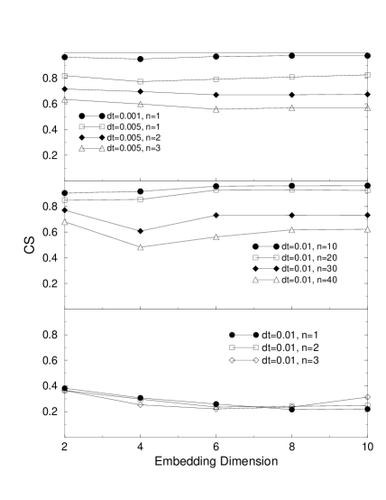
FIG. 5.: Dependence of the CS on the sampling time for different continuous-time systems. Upper panel: Lorenz system; Central panel: Standard Mackey-Glass equation (Eq. (27)); Lower panel: Random system of Eq. (8). The symbol dt indicates the time step used in the numerical integration scheme (fourth-order Runge-Kutta for the first two and Euler’s for the random system) while $n$ corresponds to the re-sampling step.

REFERENCES

- [1] G. Sugihara and R. May, Nature (London) 344, 734 (1990).
- [2] D.T. Kaplan and L. Glass, Phys. Rev. Lett. 68, 427 (1992); Physica D 64, 431 (1993).
- [3] R. Wayland, D. Bromley, D. Pickett and A. Passamante, Phys. Rev. Lett. 70, 580 (1993).
- [4] L.W. Salvino and R. Cawley, Phys. Rev. Lett. 73, 1091 (1994).
- [5] J. Bhattacharya and P. P. Kanjil, Physica D 132, 100 (1999).
- [6] H. Kantz and T. Schreiber, Nonlinear Time Series Analysis (Cambridge University Press, Cambridge, 1997).
- [7] H. Abarbanel, R. Brown, J. Sidorowich and L. Tsimring, Rev. Mod. Phys. 65, 1331 (1993).
- [8] M. Cencini, M. Falcioni, E. Olbrich, H. Kantz and A. Vulpiani, Phys. Rev. E 62, 427 (2000).
- [9] J. Jeong, M.S. Kim and S.Y. Kim, Phys. Rev. E 60, 831 (1999).
- [10] M. Casdagli, S. Eubank, D. Farmer and J. Gibson, Physica D 51, 52 (1991).
- [11] G. J. Ortega and E. Louis, Phys. Rev. Lett. 81, 4345 (1998).
- [12] G. J. Ortega and E. Louis, Phys. Rev. E. 62, 3419 (2000).
- [13] L. M. Pecora, T. L. Carroll and J. F. Heagy, Phys. Rev. E. 52, 3420 (1995).
- [14] M. Ding et al. Physica D 69, 404 (1993).
- [15] A. Galka, T. Maab and G. Pfister, Physica D 121, 237 (1998).
- [16] C. Degli Esposti Boschi, G. Ortega and E. Louis, submitted to Physica D.
- [17] R. Hegger, M. J. Bünner, H. Kantz and A. Giaquinta, Phys. Rev. Lett. 81, 558 (1998).
- [18] E. Olbrich and H. Kantz, Phys. Lett. A 232(1-2), 63 (1997).
- [19] J. Theiler, S. Eubank, A. Longtin, B. Galdrikian and J. D. Farmer, Physica D 58, 77 (1992).
- [20] T. Schreiber and A. Schmitz, Phys. Rev. Lett. 77, 635 (1996).
- [21] R. Hegger, H. Kantz and T. Schreiber, Chaos 9, 413 (1999).
- [22] A. Osborne and A. Provenzale, Physica D 35, 357 (1989).
- [23] T. Schreiber, Phys. Rev. Lett 80, 2105 (1998).