Lyapunov instability for a periodic Lorentz gas
thermostated by deterministic scattering

Abstract

In recent work a deterministic and time-reversible boundary thermostat called thermostating by deterministic scattering has been introduced for the periodic Lorentz gas [Phys. Rev. Lett. 84, 4268 (2000)]. Here we assess the nonlinear properties of this new dynamical system by numerically calculating its Lyapunov exponents. Based on a revised method for computing Lyapunov exponents, which employs periodic orthonormalization with a constraint, we present results for the Lyapunov exponents and related quantities in equilibrium and nonequilibrium. Finally, we check whether we obtain the same relations between quantities characterizing the microscopic chaotic dynamics and quantities characterizing macroscopic transport as obtained for conventional deterministic and time-reversible bulk thermostats.

PACS numbers: 05.45.Ac, 05.60.-k, 05.10.-a, 05.70.Ln

I Introduction

The investigation of nonequilibrium transport processes in many-particle systems generally requires to model the interaction between a particle and a thermal reservoir. A common approach for such a modeling are deterministic and time-reversible thermostats [1, 2, 3, 4]. Conventional types of them, such as the Gaussian and the Nosé-Hoover thermostat, are based on introducing a momentum dependent friction coefficient into the microscopic equations of motion [5, 6, 7, 8, 9]. Though the microscopic equations of motion of these systems are time-reversible the macroscopic dynamics is irreversible in nonequilibrium leading to momentum and energy fluxes with well-defined transport coefficients [5, 6, 10, 11, 12, 13, 14], which appears to be a paradox. However, investigations of the microscopic dynamics with methods from dynamical system theory could resolve this paradox by showing that the microscopic dynamics is nonlinear and highly unstable [12, 14] and leads to a phase space volume contraction onto a fractal attractor [11, 15, 16]. From the analysis of conventional thermostats, further relations between quantities characterizing the microscopic dynamics and quantities characterizing macroscopic transport could be established. At the heart of such relations there is an identity between phase space volume contraction and thermodynamic entropy production. On the basis of this identity the Lyapunov exponents could be related to the transport coefficients of a system, which has been formulated as the Lyapunov sum rule [11, 17, 18, 19, 20, 21].

These characteristic features of thermostated many-particle systems have been recovered for specific one-particle systems, the Gaussian thermostated periodic Lorentz gas [11, 15, 18, 19, 21, 22, 23, 24] and the Nosé-Hoover thermostated periodic Lorentz gas [25]. The periodic Lorentz gas consists of a particle that moves through a triangular lattice of hard disks and is elastically reflected at each disk collision. It serves as a standard model in the field of chaos and transport [14, 26]. The advantage of a one-particle system is that it reflects more strongly and transparently the nonequilibrium properties induced by a thermostat. For this reason the Lorentz gas appears as an appropriate tool to compare the properties of nonequilibrium steady states obtained from different deterministic and time-reversible thermostating mechanisms. The study of different models describing the interaction between particles and thermal reservoir and the identification of their common properties is crucial to obtain a general characterization of nonequilibrium steady states.

To investigate whether the nonequilibrium properties of conventional deterministic and time-reversible thermostats are of general validity, or just characterize these specific types of systems, an alternative deterministic and time-reversible thermostat called thermostating by deterministic scattering has been introduced for the periodic Lorentz gas [4, 27]. This thermostat is based on specifically modeling the energy transfer related to a microscopic collision process between particle and disk, where the disk mimics a thermal reservoir with infinitely many degrees of freedom. In nonequilibrium under an external electric field this mechanism leads to an on average constant kinetic energy of the particle resulting in a nonequilibrium steady state. Furthermore, the phase space volume contracts onto an attractor similar to the multifractal attractor found for the Gaussian thermostated Lorentz gas. However, differences appear in the bifurcation diagram and in the field dependence of the conductivity. This alternative thermostat has later been applied to a heat and shear flow [28].

In this work we focus on the microscopic properties of thermostating by deterministic scattering in the periodic Lorentz gas by numerically calculating the Lyapunov exponents. As quantities from dynamical systems theory, Lyapunov exponents allow a detailed characterization of the microscopic stability. In particular, they will enable us to check the general validity of relations between quantities from dynamical systems theory and statistical mechanics as obtained for conventional deterministic and time-reversible thermostats. We first explain the algorithm to calculate the Lyapunov exponents for the Lorentz gas as thermostated by deterministic scattering. Numerical computations will then show that the standard Gram-Schmidt orthonormalization has to be modified resulting in a variant of this method called constraint orthonormalization. Beside the results for the Lyapunov exponents we present results for the Kaplan-Yorke dimension and for the phase space volume contraction. We compare these results as obtained for our model with the results as known for the Gaussian thermostated Lorentz gas [21, 29], and with results for a heat and shear flow thermostated by deterministic scattering [30]. Finally, we check whether the phase space volume contraction is equal to the thermodynamic entropy production and whether the Lyapunov sum rule holds for our mechanism.

II Algorithm for the calculation of the Lyapunov exponents

In a smooth $d$-dimensional system the equations of motion for a phase space vector ${\bf\Gamma}$,

$\displaystyle\dot{\bf\Gamma}={\bf F}({\bf\Gamma})\;,$

and the corresponding equations of motion for $d$ tangent vectors ${\mbox{\boldmath$\delta$}\bf\Gamma}=({\mbox{\boldmath$\delta$}\bf r},{\mbox{\boldmath$\delta$}\bf v})$,

$\displaystyle\dot{\mbox{\boldmath$\delta$}\bf\Gamma}=\frac{\partial{\bf F}}{\partial{\bf\Gamma}}{\mbox{\boldmath$\delta$}\bf\Gamma}\;,$

are integrated to obtain $d$ Lyapunov exponents

$$\lambda=\lim_{t\to\infty}\frac{1}{t}\ln\frac{|{\mbox{\boldmath$\delta$}\bf\Gamma}(t)|}{|{\mbox{\boldmath$\delta$}\bf\Gamma}(0)|}\;.$$ (1)

The Lyapunov exponents are a measure to characterize the stability of the dynamics [31, 32]. The maximal Lyapunov exponent $\lambda$ measures the maximal exponential divergence of two initially neighboring points ${\mbox{\boldmath$\delta$}\bf\Gamma}(0)$. However, during the time evolution every tangent vector will move into the fastest growing direction due to the instability of the dynamics. All these vectors will thus become indistinguishable and their norm will diverge. The algorithm of Benettin avoids this problem by a periodic Gram-Schmidt reorthonormalization of the tangent vectors thus enabling to compute the full spectrum of Lyapunov exponents associated to the $d$-dimensional phase space [33, 34].

In the periodic Lorentz gas the time-continuous flow describing the dynamics of a phase space volume vector ${\bf\Gamma}$ in the bulk is interrupted by a time-discrete map ${\bf M}$ describing the transformation of ${\bf\Gamma}$ at the moment of a collision,

$\displaystyle{\bf\Gamma^{\prime}}={\bf M}({\bf\Gamma})\,.$

Dellago and coworkers have developed an algorithm to calculate the Lyapunov exponents for particle systems with hard sphere interactions and applied it to the Gaussian thermostated Lorentz gas [21, 29, 35]. Here the tangent vectors are transformed at the moment of a collision according to the following rule [29]:

$${\mbox{\boldmath$\delta$}\bf{\Gamma^{\prime}}}=\frac{\partial{\bf M}}{\partial{\bf\Gamma}}{\mbox{\boldmath$\delta$}\bf\Gamma}+\left[\frac{\partial{\bf M}}{\partial{\bf\Gamma}}{\bf F}({\bf\Gamma})-{\bf F}({\bf M}({\bf\Gamma}))\right]\delta\tau_{c}\,.$$ (2)

Eq. (2) is valid for arbitrary systems composed of a flow ${\bf F}$ and a time-discrete map ${\bf M}$. It takes into account that a trajectory and a satellite trajectory collide with the disk at different space points and with a time delay $\delta\tau_{c}$,

$\displaystyle\delta\tau_{c}=-\frac{({\mbox{\boldmath$\delta$}\bf r},{\bf n})}{({\bf v},{\bf n})}\;,$

where ${\bf n}$ is the unit vector perpendicular to the surface at the collision point.

Before we establish the equations of motions for the tangent vectors of the Lorentz gas as thermostated by deterministic scattering we briefly summarize the full equations of motion of Refs. [4, 27] for a particle described by the phase space vector ${\bf\Gamma}=({\bf r},{\bf v})$. In the bulk ${\bf\Gamma}$ evolves according to

$${\bf r} = \mbox{\boldmath$\varepsilon$}\frac{t^{2}}{2}+{\bf v}t+{\bf r_{0}}$$ (3)

$${\bf v} = \mbox{\boldmath$\varepsilon$}t+{\bf v_{0}}$$ (4)

where $\varepsilon$ is an external electric field of strength $\varepsilon=|\mbox{\boldmath$\varepsilon$}|$ generating a nonequilibrium situation. The basic idea of thermostating by deterministic scattering is now that at a collision energy is transfered such that the resulting velocity distribution for the particle is canonical in equilibrium. In a way, it results in a deterministic and time-reversible formulation of stochastic boundary conditions [27, 28]. For this purpose the collision rules have been defined as follows: The velocity of the particle and its direction of flight are changed at a collision with the disk according to

$$(\gamma^{\prime},v^{\prime})=(X^{-1},Y_{\infty}^{-1})\circ{\bf B}\circ(X(\gamma),Y_{\infty}(v))\;,$$ (5)

where $\gamma$ is the angle of incidence, $X(\gamma)=\sin|\gamma|$, ${\bf B}$ is the baker map [31], and

$$Y_{\infty}(v)=-\sqrt{\frac{2}{\pi T}}ve^{\frac{-v^{2}}{2T}}+\mbox{erf}(\frac{v}{\sqrt{2T}})$$ (6)

with $T$ as a parameter corresponding to the temperature of the particle $T=<v^{2}>/2$ at $\varepsilon=0$ in equilibrium. The geometry of the periodic Lorentz gas and the relevant variables are shown in Fig. 1. To ensure that the system is time-reversible, the forward baker map ${\bf B}$ acts if $0\leq\gamma\leq\pi/2$, and ${\bf B}$ is replaced by its inverse ${\bf B^{-1}}$ if $-\pi/2\leq\gamma<0$. To avoid any symmetry breaking induced by this combination of forward and backward baker map, we alternate their application in $\gamma$ with respect to the position $\beta$ of the colliding particle on the circumference. For the spacing between two neighboring disks with the radius $R=1$ we choose, following the literature [11, 21], $w\simeq 0.2361$. Investigating this system in nonequilibrium by switching on an external electric field $\varepsilon>0$ leads to a nonequilibrium steady state with on average constant kinetic energy of the particle $<v^{2}>=const.$, i. e. the system is thermostated.

The equations of motion for the tangent vectors ${\mbox{\boldmath$\delta$}\bf\Gamma}$ in the bulk can now be derived from Eqs. (4) as

$\displaystyle\left(\begin{array}[]{c}{\mbox{\boldmath$\delta$}\bf r^{\prime}}\\ {\mbox{\boldmath$\delta$}\bf v^{\prime}}\end{array}\right)=\left(\begin{array}[]{cc}1&t\\ 0&1\end{array}\right)\left(\begin{array}[]{c}{\mbox{\boldmath$\delta$}\bf r}\\ {\mbox{\boldmath$\delta$}\bf v}\end{array}\right)\;.$

The transformation rules for the tangent vectors at the moment of a collision are obtained by inserting the collision rules for the phase space vector ${\bf\Gamma}$ of Eq. (5) into Eq. (2),

$$\left(\begin{array}[]{c}{\mbox{\boldmath$\delta$}\bf r^{\prime}}\\ {\mbox{\boldmath$\delta$}\bf v^{\prime}}\end{array}\right)=\left(\begin{array}[]{cc}{\bf 1}&{\bf 0}\\ {\bf A}&{\bf B}\end{array}\right)\left(\begin{array}[]{c}{\mbox{\boldmath$\delta$}\bf r}\\ {\mbox{\boldmath$\delta$}\bf v}\end{array}\right)+\left[\left(\begin{array}[]{cc}{\bf 1}&{\bf 0}\\ {\bf A}&{\bf B}\end{array}\right)\left(\begin{array}[]{c}{\bf v}\\ \mbox{\boldmath$\varepsilon$}\end{array}\right)-\left(\begin{array}[]{c}{\bf v^{\prime}}\\ \mbox{\boldmath$\varepsilon$}\end{array}\right)\right]\delta\tau_{c}\;,$$ (7)

where

$\displaystyle A_{ij}=\frac{\partial{v_{i}}^{\prime}}{\partial r_{j}}\hskip 28.45274pt\mbox{and}\hskip 28.45274ptB_{ij}=\frac{\partial{v_{i}}^{\prime}}{\partial v_{j}}\;.$

The components of the submatrix $A$ read

$$\frac{\partial{v_{x}}^{\prime}}{\partial r_{x}} = \frac{r_{y}{v_{y}}^{\prime}}{r^{2}}[-h_{1}+1]$$

$$\frac{\partial{v_{y}}^{\prime}}{\partial r_{x}} = \frac{r_{y}{v_{x}}^{\prime}}{r^{2}}[h_{1}-1]$$

$$\frac{\partial{v_{x}}^{\prime}}{\partial r_{y}} = \frac{r_{x}{v_{y}}^{\prime}}{r^{2}}[h_{1}-1]$$

$$\frac{\partial{v_{y}}^{\prime}}{\partial r_{y}} = \frac{r_{x}{v_{x}}^{\prime}}{r^{2}}[-h_{1}+1]\,$$

and the components of the submatrix $B$ are

$$\frac{\partial{v_{x}}^{\prime}}{\partial v_{x}} = \frac{v_{y}{v_{y}}^{\prime}}{v^{2}}h_{1}+v_{x}{v_{x}}^{\prime}h_{2}$$

$$\frac{\partial{v_{y}}^{\prime}}{\partial v_{x}} = -\frac{v_{y}{v_{x}}^{\prime}}{v^{2}}h_{1}+v_{x}{v_{y}}^{\prime}h_{2}$$

$$\frac{\partial{v_{x}}^{\prime}}{\partial v_{y}} = -\frac{v_{x}{v_{y}}^{\prime}}{v^{2}}h_{1}+v_{y}{v_{x}}^{\prime}h_{2}$$

$$\frac{\partial{v_{y}}^{\prime}}{\partial v_{y}} = \frac{v_{x}{v_{x}}^{\prime}}{v^{2}}h_{1}+v_{y}{v_{y}}^{\prime}h_{2}\,$$

with

$\displaystyle h_{1}=m_{1}\frac{v^{\prime}}{v}\frac{({\bf r},{\bf v})}{({\bf r},{\bf v^{\prime}})}$

$\displaystyle h_{2}=m_{2}\frac{v}{v^{\prime 3}}\rm{e}^{-\frac{v^{\prime 2}-v^{2}}{2T}}\,.$

$\{m_{1},m_{2}\}$ are the slopes of the baker map $\{2,0.5\}$, or the slopes of the inverse baker map $\{0.5,2\}$, respectively.

In the periodic Lorentz gas as thermostated by deterministic scattering the dynamics of four orthonormal tangent vectors has to be investigated to obtain four Lyapunov exponents which completely characterize the stability in the four-dimensional phase space. Before we present our results for the Lyapunov spectrum we wish to derive explicit expressions for two other interesting quantities.

III Phase space volume contraction

The phase space volume contraction $P$ is equal to the sum of the Lyapunov exponents [32, 36],

$$P=\sum_{i}\lambda_{i}\;.$$ (8)

In the periodic Lorentz gas as thermostated by deterministic scattering only the change of a phase space volume element ${\mbox{\boldmath$\delta$}\bf\Gamma}$ at the moment of a collision as described by Eq. (7) contributes to $P$. The mean exponential rate of the phase space volume contraction $P$ can then be calculated according to

$$P=<\ln\left|\frac{\partial{\mbox{\boldmath$\delta$}\bf\Gamma^{\prime}}}{\partial{\mbox{\boldmath$\delta$}\bf\Gamma}}\right|>\;,$$ (9)

where

$\displaystyle\left|\frac{\partial{\mbox{\boldmath$\delta$}\bf\Gamma^{\prime}}}{\partial{\mbox{\boldmath$\delta$}\bf\Gamma}}\right|=\left|\begin{array}[]{cc}\frac{\partial{\mbox{\boldmath$\delta$}\bf r^{\prime}}}{\partial{\mbox{\boldmath$\delta$}\bf r}}&{\bf 0}\\ \frac{\partial{\mbox{\boldmath$\delta$}\bf v^{\prime}}}{\partial{\mbox{\boldmath$\delta$}\bf r}}&\frac{\partial{\mbox{\boldmath$\delta$}\bf v^{\prime}}}{\partial{\mbox{\boldmath$\delta$}\bf v}}\end{array}\right|=\left(\frac{\partial\delta{r_{x}}^{\prime}}{\partial\delta r_{x}}\frac{\partial\delta{r_{y}}^{\prime}}{\partial\delta r_{y}}-\frac{\partial\delta{r_{x}}^{\prime}}{\partial\delta r_{y}}\frac{\partial\delta{r_{y}}^{\prime}}{\partial\delta r_{x}}\right)\left(\frac{\partial\delta{v_{x}}^{\prime}}{\partial\delta v_{x}}\frac{\partial\delta{v_{y}}^{\prime}}{\partial\delta v_{y}}-\frac{\partial\delta{v_{x}}^{\prime}}{\partial\delta v_{y}}\frac{\partial\delta{v_{y}}^{\prime}}{\partial\delta v_{x}}\right)\;.$

The partial derivatives of Eq. (7) read

$$\frac{\partial\delta{r_{x}}^{\prime}}{\partial\delta r_{x}} = 1+({v_{x}}^{\prime}-v_{x})\frac{n_{x}}{({\bf v},{\bf n})}$$

$$\frac{\partial\delta{r_{y}}^{\prime}}{\partial\delta r_{x}} = ({v_{x}}^{\prime}-v_{x})\frac{n_{y}}{({\bf v},{\bf n})}$$

$$\frac{\partial\delta{r_{x}}^{\prime}}{\partial\delta r_{y}} = ({v_{y}}^{\prime}-v_{y})\frac{n_{x}}{({\bf v},{\bf n})}$$

$$\frac{\partial\delta{r_{y}}^{\prime}}{\partial\delta r_{y}} = 1+({v_{y}}^{\prime}-v_{y})\frac{n_{y}}{({\bf v},{\bf n})}\,$$

$$\frac{\partial\delta{v_{x}}^{\prime}}{\partial\delta v_{x}} = B_{00}$$

$$\frac{\partial\delta{v_{y}}^{\prime}}{\partial\delta v_{x}} = B_{10}$$

$$\frac{\partial\delta{v_{x}}^{\prime}}{\partial\delta v_{y}} = B_{01}$$

$$\frac{\partial\delta{v_{y}}^{\prime}}{\partial\delta v_{y}} = B_{11}\;.$$

Inserting these expressions into Eq. (9) yields

$$P=\frac{<v^{\prime 2}>-<v^{2}>}{2T}\;.$$ (10)

The phase space volume contraction depends thus only on the average transfer of kinetic energy to the reservoir. Equation (10) is valid in equilibrium as well as in nonequilibrium. An analogous result has been obtained for collisions with a flat wall in a heat and shear flow thermostated by deterministic scattering [28], however, in case of shear the expression for $P$ turned out to be more complicated.

If $P<0$ the phase space volume typically contracts onto a fractal attractor in the driven periodic Lorentz gas [11, 15, 16]. The geometric properties of the attractor can be related to the Lyapunov exponents by the Kaplan-Yorke conjecture, $D_{KY}=D_{1}$. Here $D_{1}$ is the information dimension [31] and $D_{KY}$ is the Kaplan-Yorke dimension defined by

$$D_{KY}=j+\frac{\sum_{i=1}^{j}\lambda_{i}}{|\lambda_{j+1}|}\;,$$ (11)

where the $\lambda_{i}$ are ordered by magnitude, $\lambda_{1}>\lambda_{2}>\ldots$, and $j$ is the largest integer for which $\sum_{i=1}^{j}\lambda_{i}>0$.

IV Thermodynamic entropy production and reservoir temperature

The macroscopic properties of nonequilibrium steady states can be characterized by quantities from thermodynamics and statistical physics. In this work we want to check whether we can relate the thermodynamic entropy production $dS$,

$$dS=\frac{dQ}{T_{r}}\;,$$ (12)

to the phase space volume contraction. To calculate the thermodynamic entropy production for thermostating by deterministic scattering we have to calculate the temperature of the reservoir $T_{r}$ in nonequilibrium. As discussed in Ref. [27], in nonequilibrium the temperature related to the particle, or respectively the temperature in the bulk $T_{b}$ defined via equipartitioning of energy, is greater than the parametric temperature $T$ in Eq. (6) and increases with the field strength. Moreover, $T_{b}$ is inhomogeneously distributed in the bulk because the thermostat acts only at the boundary. In this subsection we derive an expression for the temperature of the reservoir $T_{r}$ similarly to how it has been done in Ref. [28].

If we assume equipartitioning of energy of particle and reservoir at the wall, we can define the reservoir temperature $T_{r}$ indirectly via the velocity distribution of the particle at the moment of the collision denoted as $\varrho_{map}$. For sake of simplicity, here we do not explicitly consider the dependence of $T_{r}$ on the position $\beta$ of the colliding particle at the disk. An expression for the temperature of the reservoir can then be derived from the temperature in the bulk on the basis of the relation between the map density $\varrho_{map}$ and the time-continuous density $\varrho$ in the bulk as given by Eq. (5) in Ref. [27],

$$\varrho(v)=const.\frac{\varrho_{map}(v)}{v}\;.$$ (13)

The precise derivation of this equation can be found in Sect. IIIB2 of Ref. [27]. To obtain the expressions for the velocity fluctuations parallel and perpendicular to the reservoir, the corresponding equations for the velocity distributions of the normal and tangential components $v_{n}$ and $v_{t}$, respectively, have to be calculated. For this purpose, first the analogous equation for $\varrho(\gamma)$ corresponding to Eq. (13) must be derived. Knowing that in equilibrium $\varrho(\gamma)=1$ because of symmetry and $\varrho_{map}(\gamma)=\cos\gamma$ at the disk leads to

$$\varrho(\gamma)=const.\frac{\varrho_{map}(\gamma)}{|\cos(\gamma)|}\;.$$ (14)

Combining these two equations yields the full transformation

$\displaystyle\varrho(v)\varrho(\gamma)=\frac{const.}{v|\cos(\gamma)|}\varrho_{map}(v)\varrho_{map}(\gamma)\;.$

Changing to local Cartesian coordinates $(v_{n},v_{t})$ co-rotating with the position $\beta$ at the disk and applying the transformation $dv_{n}dv_{t}=vdvd\gamma$ results in

$$\varrho(v_{n})\varrho(v_{t})=\frac{const.}{v|\cos(\gamma)|}\varrho_{map}(v_{n})\varrho_{map}(v_{t})$$ (15)

Noting that $|v_{n}|=v|\cos(\gamma)|$ and matching the variables on both sides, Eq. (15) can be decomposed into

$$\varrho(v_{t})=\varrho_{map}(v_{t})$$ (16)

with $-\infty<v_{t}<\infty$ and

$$\varrho(v_{n})=\frac{const.}{|v_{n}|}\varrho_{map}(v_{n})$$ (17)

with $0<v_{n}<\infty$. Before we come to the reservoir temperature definitions which are based on these densities, we remark that the disk which serves as the thermal reservoir is fixed and cannot recognize any current. In other words, only the kinetic energy of the particle in the fixed frame of the bulk $2E_{pf}=<v^{2}>$ is relevant for the interaction with the reservoir, and no average current needs to be subtracted. Defining now $[\ldots]$ as the average over $\varrho_{map}$ Eq. (16) implies for the tangential component $<v_{t}^{2}>=[v_{t}^{2}]$ thus leading to the definition of $T_{t}$ as

$\displaystyle T_{t}=\frac{[v_{t}^{2}]+[v_{t}^{\prime 2}]}{4}\;.$

Analogously, the average over the map density corresponding to $<v_{n}^{2}>$ can be calculated from Eq. (17) to

$\displaystyle<v_{n}^{2}>=\frac{\int_{-\infty}^{\infty}v_{n}^{2}\varrho(v_{n})dv_{n}}{\int_{-\infty}^{\infty}\varrho(v_{n})dv_{n}}=\frac{\int_{-\infty}^{\infty}|v_{n}|\varrho_{map}(v_{n})dv_{n}}{\int_{-\infty}^{\infty}\frac{1}{|v_{n}|}\varrho_{map}(v_{n})dv_{n}}=\frac{[|v_{n}|]}{[\frac{1}{|v_{n}|}]}\;,$

where the denominator is obtained from joint normalization over the ingoing and outgoing fluxes. $T_{n}$ is then defined as

$\displaystyle T_{n}=\frac{1}{2}\frac{[|v_{n}|+v_{n}^{\prime}]}{[\frac{1}{|v_{n}|}+\frac{1}{v_{n}^{\prime}}]}$

with $-\infty<v_{n}\leq 0$ and $0\leq v_{n}^{\prime}<\infty$.

The total temperature of the reservoir $T_{r}$ is consequently the average of $T_{t}$ and $T_{n}$,

$$T_{r}=\frac{T_{t}+T_{n}}{2}\;.$$ (18)

$T_{r}$ can be calculated as an average over $\beta$ or locally in a small interval $\Delta\beta$. We note that our result for $T_{n}$ is slightly different to the result in Ref. [28], which strictly speaking is only valid if the in- and outgoing densities are symmetrical.

This definition of the temperature is exact in equilibrium, however, in case of a nonequilibrium situation Eq. (13) and Eq. (14) are not valid anymore. A more detailed analysis of these shortcomings leads to the conclusion that $T_{r}$ calculated according to Eq. (18) will be greater than the real temperature of the reservoir for higher field strength [37]. One would only obtain the real temperature of the reservoir if one would use the correct relation between map density and time-continuous density in nonequilibrium, and this is not known. In any case, a lower bound for the temperature of the reservoir which we denote as $T_{lr}$ can be calculated by only taking into account the velocity of the particle after a collision.

V Equilibrium

The numerical calculation of the Lyapunov spectrum for the Lorentz gas as thermostated by deterministic scattering according to the method presented in section II leads to the following result in equilibrium: $\{\lambda\}=\{1.8695,0.0104,-0.0104,-1.8695\}$. These data appear to be at variance with the fact that in equilibrium two zero Lyapunov exponents have to exist, one associated with the direction of the flow, and a second one resulting from the conjugate pairing rule in equilibrium [32]. We have performed the following tests to detect the reason for this discrepancy:

1. We have numerically calculated the Lyapunov exponents by investigating the dynamics of a trajectory and four satellite trajectories, i. e., for finite but small distances. The Lyapunov spectrum obtained by this method was the same.

2. Changing parameters like the interdisk distance $w$, the parametric temperature $T$, the dimensionality of the reservoir [4, 27], the slope of the baker map, and replacing the baker map by more complicated two-dimensional maps like the cat map or the standard map [31] did not improve the result.

3. We have followed the temporal evolution of two points on the same trajectory for about 20 collisions without orthonormalization and by choosing as initial conditions a) that the points are slightly displaced along the trajectory but have the same velocity, b) that the points have the same configuration space coordinates but slightly different velocities. We could then show that two neutral directions exist corresponding to a) the direction of the flow and b) to one direction perpendicular to the flow.

The third test indicates that two zero Lyapunov exponents indeed exist. Thus, there must be a numerical problem because of standard Gram-Schmidt orthonormalization which establishes an orthonormal system of the tangent vectors on the basis of the most unstable direction. To cure that problem, we propose an alternative method to perform the periodic orthonormalization. This method establishes an orthonormal system of the tangent vectors starting from the existing neutral direction of the flow. Since we are introducing an additional constraint this way we call it constraint orthonormalization. It consists of the following steps:

1. Choose suitable initial conditions for the orthonormal system: The first tangent vector is situated in the direction of the flow, ${\mbox{\boldmath$\delta$}\bf\Gamma_{1}}=(v_{x0}/v_{0},v_{y0}/v_{0},0,0)$, and the other tangent vectors are orthonormal to it.

2. At every orthonormalization the first tangent vector is forced to point in the direction of the flow, ${\mbox{\boldmath$\delta$}\bf\Gamma_{1}}=(v_{x}/v,v_{y}/v,0,0)$. This step corrects the very small deviations of the first tangent vector from the direction of the flow resulting from a collision with the disk, as will be explained in more detail below.

3. The second, third and fourth tangent vector are orthonormalized again starting from the first one according to the method of Gram-Schmidt.

The application of constraint orthonormalization leads to the following Lyapunov spectrum in equilibrium: $\{\lambda\}=\{1.8695,0.0000,0.0000,-1.8695\}$, see also Fig. 3. Comparing these results to the previous ones obtained from the standard method shows that the Gram-Schmidt orthonormalization led to a wrong result only for the second and third Lyapunov exponent. The explanation for this numerical problem is as follows: In equilibrium the average energy transfer to the reservoir is zero. Still, at any collision energy is transfered either from the particle to the reservoir or in the opposite direction. According to Eq. (10) the phase space volume thus locally contracts or expands although the global phase space volume contraction is zero. However, as shown by Eq. (8) the phase space contraction is intimately related to the corresponding (un)stable directions in phase space. Consequently, the local contractions and expansions at a collision change the orientation and the norm of the tangent vectors in a nontrivial way. The Gram-Schmidt orthonormalization reacts to these changes by turning the corresponding tangent vectors out of the previously neutral directions. The problem why the Gram-Schmidt procedure does not converge to the existing two neutral directions at least in the long time limit could not be completely resolved even by very detailed numerical investigations of the dynamics. Possibly some kind of resonance phenomenon between local phase space contraction and expansion at the collision and Gram-Schmidt orthonormalization after the collision leads to the corresponding tangent vectors adjusting themselves somewhat symmetrically around these two neutral directions [38].

In summary, constraint orthonormalization correctly yields a second zero Lyapunov exponent beside the zero Lyapunov exponent corresponding to the constrained direction of the flow. In agreement with the on average zero energy transfer between particle and reservoir the sum of the Lyapunov exponents and the global phase space volume contraction are zero. Furthermore, the Lyapunov exponents trivially fulfill the conjugate pairing rule related to the Hamiltonian character of the dynamics in equilibrium. The probability density in the Lorentz gas cell is uniform in equilibrium and, as a consequence, the Kaplan-Yorke dimension is equal to the dimension of the phase space, $D_{KY}=d=4$. In addition, the parametric temperature $T$, the temperature in the bulk $T_{b}$, and the reservoir temperature $T_{r}$, are all equal, $T=T_{b}=T_{r}$.

We now turn to an even more detailed analysis of the dynamical instability of our model system by following ideas summarized in Refs. [36, 39]. If a dynamical system is ergodic, the Lyapunov exponents do not depend on the initial conditions of the tangent vectors, and thus they only yield information about the global instability. This implies that Eq. (1) provides no direct way to assess the local instability of the system at specific values of phase space variables like the angle of incidence at a disk $\gamma$ and the position of the colliding particle $\beta$. In Refs. [36, 39], two slightly different ways have been proposed how to access information on local instabilities depending on these parameters. Here we use the approach proposed in Ref. [39] which characterizes the local deformation of a typical tangent vector $\delta{\bf\Gamma}$ at the moment of a collision by introducing the quantity

$$\lambda_{c}(\sin\gamma,\beta)=<\ln\frac{|\delta\bf\Gamma^{\prime}|}{|\delta\bf\Gamma|}>\;,$$ (19)

where the brackets indicate an average over all collisions in a respective small interval around $\beta$ and/or $\gamma$. The physical motivation for defining this quantity is that any tangent vector quickly orients itself into the direction of fastest growth. Accordingly, the full memory about the maximum instability of the system is contained in the orientation of the tangent vector thus representing a “needle” in phase space which very sensitively measures the local changes of the stability at a collision. Therefore, this quantity is a very sensitive function of $\gamma$ and $\beta$. In Ref. [39] this quantity has been called a local Lyapunov exponent, however, this term has also been used in the literature to indicate the dependence of the Lyapunov exponents Eq. (1) on initial conditions in case the dynamics is non-ergodic [32]. To avoid possible confusion, and by following Ref. [36] where very related quantities have been defined, here we denote $\lambda_{c}$ as the local stretching rates of the system. Note that the clever and very simple definition by Eq. (19) makes at least the maximum local stretching rate directly accessible to computer simulations. In contrast, in Ref. [36] the full spectrum of these rates has been defined in a proper co-moving coordinate system. This makes their definition more convenient in mathematical terms, but also less accessible for straightforward numerical computations. Both these different definitions are related via coordinate transformations [40]. Unfortunately, local stretching rates are not coordinate-invariant thus yielding different values depending on their precise definition, even in conjugate dynamical systems.

$\lambda_{c}$ as a function of $\beta$ for thermostating by deterministic scattering in comparison to elastic collisions is presented in Fig. 2(a) showing that the conventional hard disk Lorentz gas and our thermostated version of it share the same properties. The maxima/minima of $\lambda_{c}(\beta)$ correspond to the directions of maximal/minimal distances between neighboring disks, respectively. Results for the conventional Lorentz gas in a more detailed view of phase space, i.e., $\lambda_{c}(\sin(\gamma))$ for $|\beta|<0.00001$ as presented in Ref. [39], have shown that the local stretching rate $\lambda_{c}$ is a singular function of $\sin(\gamma)$ (see also Ref. [36]). Related results for $\lambda_{c}(\sin(\gamma))$ for the Lorentz gas as thermostated by deterministic scattering are presented in Fig. 2. The curve in Fig. 2(b) looks qualitatively very similar to the curve in Fig. 1 of [39]. However, the numerical results for $\lambda_{c}(\sin(\gamma))$ of our system are not sufficiently accurate [41] to study the existing discontinuities on a finer scale, as it has been done in Fig. 2 of Ref. [39]. To perform such investigations in a slightly more detailed way we looked at the refined, decomposed local stretching rate $\lambda_{c_{\Gamma_{x}}}=<\ln(|\delta\Gamma_{x}^{\prime}|)/(|\delta\Gamma_{x}|)>$ which characterizes the deformation of the x-component of a tangent vector only. The results for $\lambda_{c_{\Gamma_{x}}}$ are presented in Figs. 2 (d) and (e). Fig. 2(e) shows an enlarged sector of (d) where one can see a roughly symmetric profile composed of maxima and minima on a fine scale. The apparent symmetry of most of these peaks suggests that these oscillations are not due to numerical errors. We consider this as an indication that for the Lorentz gas as thermostated by deterministic scattering at least the refined local stretching rate $\lambda_{c_{\Gamma_{x}}}$ could be a singular function of $\sin(\gamma)$. It may be somewhat surprising that such specific dynamical properties of the conventional, unthermostated Lorentz gas persist in our thermostated system as well. However, this leads to the conclusion that the geometric instability of the system is more important for these characteristics than the one resulting from the modifications related to our specific scattering mechanism.

VI Nonequilibrium

In nonequilibrium we choose the electric field such that $\varepsilon_{x}>0,\varepsilon_{y}=0$. The field accelerates the particle, and energy is transfered on average to the disk resulting in a nonequilibrium steady state. As a consequence, the global phase space volume contraction given by Eq. (10) is negative. The detailed dependence of the Lyapunov spectrum on the field strength is shown in Fig. 3, where both results from the standard method as well as from the constraint method are presented. Only one zero Lyapunov exponent exists in nonequilibrium associated with the direction of the flow. For higher field strength unconstraint Gram-Schmidt orthonormalization correctly turns the second tangent vector in the direction of the flow, $\lambda_{2}<10^{-4}$ for $\varepsilon_{x}>0.5$.

To obtain the correct Lyapunov exponents for $\varepsilon_{x}<0.5$ in nonequilibrium, we apply a suitably adjusted version of constraint orthonormalization as used in equilibrium: In order to achieve that two points on a trajectory stay on the same trajectory after a collision, their initial states and velocities have to be chosen such that the points have the same velocity at the moment of the collision. This condition leads to the components for the first tangent vector ${\mbox{\boldmath$\delta$}\bf\Gamma_{1}}=\{v_{x0},v_{y0},\varepsilon_{x},0\}$. Note that ${\mbox{\boldmath$\delta$}\bf\Gamma}$ is not normalized here. The other steps are then the same as in equilibrium.

The Lyapunov spectrum as a function of the field strength obtained from constraint orthonormalization is also presented in Fig. 3. As in equilibrium, the results of the two methods differ only for the second and third Lyapunov exponent for $\varepsilon_{x}<0.5$. The differences for the third Lyapunov exponent are of the same size as the differences for the second Lyapunov exponent. The second Lyapunov exponent obtained by the new method is zero for all field strengths corresponding to the constrained tangent vector in the direction of the flow. The third Lyapunov exponent decreases with increasing field strength which is related to the dominant energy transfer in the direction from the particle to the disk. The dependence of the third and of the fourth Lyapunov exponent on the field strength appears to be a power law, which is a behavior that has also been observed for the Gaussian thermostated Lorentz gas for small enough field strength [42]. According to Pesins theorem [32], the only positive Lyapunov exponent is equal to the Kolmogorov-Sinai entropy $h_{KS}$,

$\displaystyle h_{KS}=\sum_{i}\lambda_{i}^{+}\;.$

Interestingly, its curve is nonmonotonous. For small field strength, the dynamics in configuration space appears to be dominated by the fact that the trajectory of the particle is getting adjusted in the direction of the field, and the Kolmogorov-Sinai entropy decreases. For higher field strength the increasingly disordered dynamics in velocity space related to an increase of the bulk temperature $T_{b}$ seems to become more important, and the Kolmogorov-Sinai entropy increases. The same field dependence of the Kolmogorov-Sinai entropy has been observed in a shear flow as thermostated by deterministic scattering [30]. It would be interesting to know whether this is a general property appearing in field-driven system as thermostated by deterministic scattering. In contrast to this observation, the Kolmogorov-Sinai entropy monotonically decreases for the Gaussian thermostated Lorentz gas because the constraint of the bulk thermostat onto the dynamics increases with increasing field strength [21, 43]. Whether the irregularities on the fine scale in Fig. 3 are a property of the dynamics or whether they are numerical fluctuations could not be decided on the basis of the present data.

The sum of the Lyapunov exponents is negative and according to Eq. (10) equal to the phase space volume contraction $P$. As presented in Fig. 4(a), $P$ decreases with increasing field strength. The density of the attractor remains phase space filling but shows a nonuniform and complicated structure as shown in the Poincaré section in Fig. 4(a) of Ref. [4]. Therefore we can assume that the Hausdorff dimension $D_{0}$ is equal to the dimension of the phase space, $D_{0}=d=4$, as is also the case for Gaussian thermostated periodic Lorentz gases. In contrast, the Kaplan-Yorke dimension $D_{KY}$ defined by Eq. (11) is not an integer anymore, as presented in Fig. 4(c). This provides quantitative evidence for the fractal structure of the attractor according to the conjecture $D_{KY}=D_{1}$.

Some of the conventional deterministic and time-reversible bulk thermostats fulfill the conjugate pairing rule saying that the Lyapunov exponents can be grouped into pairs such that $\lambda_{+}+\lambda_{-}=const.$ [3, 20]. Fig. 4(b) shows that the conjugate pairing rule does not hold for our model. However, this does not come as a big surprise because it is well-known that even conventional thermostats do not exhibit conjugate pairing if thermostated at the boundaries [44, 26].

The local expansion rate $\lambda_{c}(\beta)$ as defined in Eq. (19) is presented in Fig. 5(b) and can be compared with $\varrho(\beta)$ shown in Fig. 5(a). One still recovers remnants of the periodic equilibrium distribution of $\lambda_{c}$, see Fig. 2(a). However, they are strongly deformed by the anisotropy induced by the field, and the maxima and minima are much more pronounced. In contrast to equilibrium, there exist two absolute maxima, one around $\beta\approx\pi/6$ and one around $\beta\approx 2\pi-\pi/6$, and an absolute minimum around $\beta\approx\pi$. The maxima and minima of $\lambda_{c}(\beta)$ occur just opposite to the maxima and minima of $\varrho(\beta)$. This is in agreement with the physical interpretation that a more unstable dynamics leads to a more dilute particle density in phase space. To extend the comparison, the temperature of the reservoir $T_{r}$ as a function of $\beta$ calculated according to Eq. (18) is presented in Fig. 5(c). The distribution of peaks in $\lambda_{c}(\beta)$ and $T_{r}(\beta)$ is very similar. This might be related to the fact that both quantities illustrate somewhat irregular behavior: $\lambda_{c}$ characterizes the instability of the dynamics and $T_{r}$ is equal to the mean kinetic energy of the degrees of freedom of the reservoir. The analogous $\beta$-dependence of $\lambda_{c}$ and $T_{r}$ points again to a close relation between dynamical system theory and statistical mechanics. At $\beta\approx\pi$ both the distributions of $\lambda_{c}$ and $T_{r}$ show a more complicated structure. This is probably a consequence of the dynamics being directed parallel to the field resulting in the global minimum of $\lambda_{c}$ on a coarse scale, whereas for other $\beta$ the dynamics is more chaotic. For more detailed views of the phase space in terms of the local stretching rate, in analogy to Fig. 2 in equilibrium, we could not get qualitative good results [41]. Thus, whether $\lambda_{c}(\beta)$ is a singular function in nonequilibrium on a fine scale remains an open question.

The dependence of $T_{r}$ on the field strength according to the definition in Eq. (18), in which $T_{r}$ is averaged over $\beta$, and the lower bound $T_{lr}$ as defined below this equation are shown in Fig. 4(d). In particular, the results for $T_{lr}(\varepsilon)$ confirm that $T_{r}$ is always greater in nonequilibrium than the parametric temperature $T$, $T_{r}>T$.

More detailed information related to the deviations between reservoir temperature and parametric temperature are obtained by studying the map densities $\varrho_{map}(v_{t})$ and $\varrho_{map}(v_{n})$ at a collision as represented in Fig. 6. The deviations between ingoing and outgoing densities in both cases are reminiscent of an average transfer of kinetic energy from particle to reservoir, as it is necessary to compensate the influx of energy caused by the electric field to obtain a nonequilibrium steady state. However, in case of the periodic Lorentz gas taking the thermodynamic limit leaves the system precisely as it is. Consequently, there is no thermodynamic way to get rid of the difference between ingoing and outgoing velocity distribution. But these differences are the dynamical reason why in nonequilibrium the reservoir temperature $T_{r}$ is typically not equal to the parametric temperature $T$, because this would only be the case if both distributions would be converging to the (local) equilibrium distribution in the thermodynamic limit, as included in these figures. This aspect will become important for understanding our results on the relation between phase space contraction and entropy production below.

In Fig. 7, the kinetic energy of the particle in the bulk averaged over $\beta$, $E_{pf}=<v^{2}>/2$, is presented as a function of the distance $d$ from the disk. The profile of $E_{pf}$ is inhomogeneous as expected. For $d\to 0$, $E_{pf}$ should approach the temperature of the reservoir defined via equipartitioning of energy thus providing an alternative definition of the reservoir temperature based on the bulk dynamics in the inner ring around the disk. However, it is not possible to safely extrapolate to this limiting value on the basis of the present data [41]. Comparing $E_{pf}$ for $d\to 0$ with $T_{r}$ shows in particular that $T_{r}>E_{pf}$ for $\varepsilon_{x}=1$ excluding convergence via extrapolation, i.e., the assumptions made in the derivation of Eq. (18) do not hold in nonequilibrium, but at least they yield a reasonable estimate. Note that the kinetic energy in this limit is still always greater than the lower bound for the reservoir temperature, $E_{pf}>T_{lr}$, which will be important for our following discussion of entropy production.

The external driving force $\varepsilon$ performs work on the system and causes a macroscopic flow characterized by a positive conductivity $\sigma>0$ [27]. At the same time, work is transformed into heat and in turn removed by the thermostat leading to a positive thermodynamic entropy production. Starting from Eq. (12), the irreversible entropy production in the bulk $dS$ is easily computed by defining the heat production $dQ$ as the change of the kinetic energy of the particle in the bulk, $dE_{pf}/dt$, and feeding in the bulk equations of motion Eq. (4). This leads to the well-known expression of entropy production via Joule heating

$$dS=\frac{\varepsilon_{x}<v_{x}>}{T_{r}}\;.$$ (20)

The numerical result for the field dependence of the thermodynamic entropy production according to this equation is presented in Fig. 4(a).

On the other hand, as discussed above the heat produced in the bulk must leave as an outward flux across the walls absorbed by the thermal reservoir. Correspondingly, computing the average change of the kinetic energy during a free flight from the equations of motion yields

$$\varepsilon_{x}<v_{x}>=\frac{<v^{2}>-<v^{\prime 2}>}{2}\;,$$ (21)

where the right hand side is just the average transfer of kinetic energy at a collision. Inserting this result into Eq. (20) leads to

$$dS=\frac{<v^{2}>-<v^{\prime 2}>}{2T_{r}}\;.$$ (22)

Comparing now Eq. (22) with Eq. (10) yields the important result that the identity between thermodynamic entropy production and phase space volume contraction does not hold for the Lorentz gas as thermostated by deterministic scattering. Instead, these two quantities just differ by the factor $T/T_{r}(\varepsilon_{x})$,

$$dS=-P\frac{T}{T_{r}(\varepsilon_{x})}\;.$$ (23)

To explicitly compare these two quantities the field dependence of $-P$ is also presented in Fig. 4(a). As we have discussed above, there is some ambiguity in defining the reservoir temperature $T_{r}$, however, we emphasize that all our applied definitions and bounds lead to the result that $-P$ and $dS$ are inherently different in nonequilibrium. This is also clear from the fact how the thermostat works in our model, as explained above.

As has been done in conventional thermostats, starting from Eq. (23) a relation between the electrical conductivity and the phase space volume contraction can now be established by using Eq. (20) and replacing the average current according to the definition of the conductivity

$\displaystyle\sigma=\frac{<v_{x}>}{\varepsilon_{x}}$

yielding

$\displaystyle\sigma=\frac{-TP}{\varepsilon^{2}_{x}}=\frac{-T\sum\lambda}{\varepsilon^{2}_{x}}\;.$

This equation is formally identical to the Lyapunov sum rule obtained for the conventional thermostats. The only difference is the constant factor $T$ which, for conventional thermostats, corresponds to the temperature of the reservoir. If the Lyapunov sum rule applies, it shows that macroscopic transport can be directly understood in terms of the microscopic dynamics characterized by the sum of the Lyapunov exponents.

However, we remark that the existence of a Lyapunov sum rule in thermostated systems being of the simple type as one above rather seems to be the exception than the rule: For example, a difference between phase space volume contraction and thermodynamic entropy production has also been obtained for a shear flow as thermostated by deterministic scattering [28]. For this system the expressions for $P$ and $dS$ can be rather complicated. Consequently, the Lyapunov sum rule does not hold, and a similar relation has not been found in addition. Furthermore, already a variation of the Nosé-Hoover and of the Gaussian thermostat did not lead to an identity between $P$ and $dS$ implying the invalidity of the Lyapunov sum rule as well, as discussed in Ref. [25, 37].

In general, the relation between phase space volume contraction and thermodynamic entropy production, and the corresponding relation between transport coefficient and Lyapunov exponents, will depend on the details of the microscopic energy transfer between particle and reservoir. Based on our studies in Refs. [4, 25, 27, 28], we conclude that an identity between $P$ and $dS$ appears only to be valid for what might be called “ideal” thermostats meaning that energy is exchanged between subsystem and reservoir by sufficiently simple coupling rules as they are provided, for example by conventional Gaussian and Nose-Hoover thermostats.

VII Conclusions

In this work we have numerically calculated the Lyapunov exponents for the Lorentz gas thermostated by deterministic scattering. The Gram-Schmidt orthonormalization, a fundamental ingredience of the standard method to calculate Lyapunov exponents, led to a wrong result for the Lyapunov spectrum by applying this thermostat. We modified this method by imposing an additional constraint, summarized as constraint orthonormalization, and found results which are in agreement with expectations from dynamical systems theory. We wish to remark that the phenomenon causing our numerical difficulties is reminiscent of an inelastic collision of a particle with a hard disk, as it is also modeled in granular materials by using restitution coefficients. Thus, applying constraint orthonormalization might be helpful for exactly computing Lyapunov spectra in low-dimensional systems of granular type as well. On the basis of the Lyapunov exponents further quantities have been calculated to characterize the nonequilibrium steady state. The comparison of the results obtained for thermostating by deterministic scattering with the ones known for conventional thermostats leads to the following conclusions:

1. The sum of the Lyapunov exponents for thermostating by deterministic scattering is negative in nonequilibrium in agreement with the phase space volume contraction onto an attractor. For thermostating by deterministic scattering only one Lyapunov exponent is zero in nonequilibrium related to the direction of the flow. Similar results could be expected for the Nosé-Hoover thermostated Lorentz gas where the calculation of the Lyapunov exponents have not yet been performed. In contrast, for the Gaussian thermostated Lorentz gas two Lyapunov exponents are zero in nonequilibrium because the thermostat keeps the kinetic energy of the particle strictly constant.

2. The Kaplan-Yorke dimension calculated on the basis of the Lyapunov exponent is not an integer in nonequilibrium providing quantitative evidence that the attractor of thermostating by deterministic scattering in the periodic Lorentz gas exhibits a fractal structure analogous to the conventional bulk thermostats.

3. The identity between thermodynamic entropy production and phase space volume contraction does not hold for thermostating by deterministic scattering. Instead, these two quantities differ by a field dependent factor. The reason for this difference is that the temperature of the reservoir of thermostating by deterministic scattering depends on the field strength, in contrast to Gaussian and Nosé-Hoover thermostats. This result is important, since this identity was accepted up to now as a general characterization of nonequilibrium steady states generated by deterministic and time-reversible thermostats.

4. Surprisingly, although there is no identity we could still establish a relation between conductivity and Lyapunov exponents for thermostating by deterministic scattering. This equation is formally identical to the Lyapunov sum rule for conventional thermostats. As far as we know, our model thus provides a first example of a system where there is no identity, but where nevertheless there is a simple relation between transport coefficients and dynamical instabilities similar to conventional thermostats.

In summary, we find that the existence of fractal attractors in nonequilibrium steady states are common features which thermostating by deterministic scattering shares with conventional thermostats. Physically speaking, the fractal character reflects the extreme rarity of nonequilibrium states relative to equilibrium ones. To look for additional common properties of all deterministic and time-reversible thermostats remains an important question, which is intimately related to obtaining a general characterization of nonequilibrium steady states. Such a characterization might result in a more general relation between quantities of thermodynamic interest and the indicators of dynamical chaos at the microscopic level, from which the relations obtained for the thermostating mechanisms considered above could appear as special cases.

Acknowledgments: We are indebted to C. Dellago for his assistance concerning the numerical calculation of the Lyapunov exponents, and we thank Prof. G. Nicolis for his ongoing support and encouragement in this research. Thanks go to J. Wiersig for helpful proof-reading. K.R. thanks the European Commission for a TMR grant under contract no. ERBFMBICT96-1193 and the foundation “D. & A. van Buuren” for financial support. R.K. wishes to acknowledge support from the MPIPKS for this work in form of a distinguished postdoctoral fellowship.

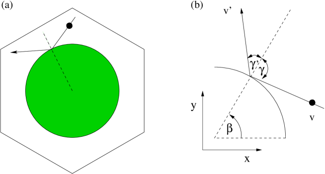
FIG. 1.: (a) Elementary cell of the periodic Lorentz gas on a triangular lattice. (b) Definition of the relevant variables.

FIG. 2.: Local stretching rate in equilibrium: (a) thermostating by deterministic scattering (solid curve), elastic collisions (dashed curve) for all $\gamma$; (b)-(e) thermostating by deterministic scattering, (b) $|\beta|<0.00001$, (c) $|\beta-\pi/2|<0.00001$; (d),(e) refined local stretching rate, (d) $|\beta-\pi/2|<0.00001$, (e) enlarged sector of (d).

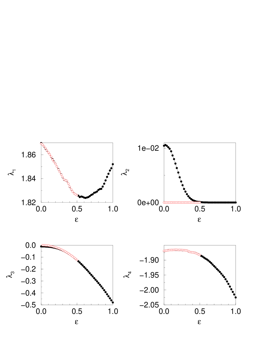
FIG. 3.: Field dependence of the four Lyapunov exponents in nonequilibrium; filled circles: Gram-Schmidt orthonormalization, empty circles: constraint orthogonalization as defined in the text. In this and in the following figures the error for the results is less then $5\cdot 10^{-4}$.

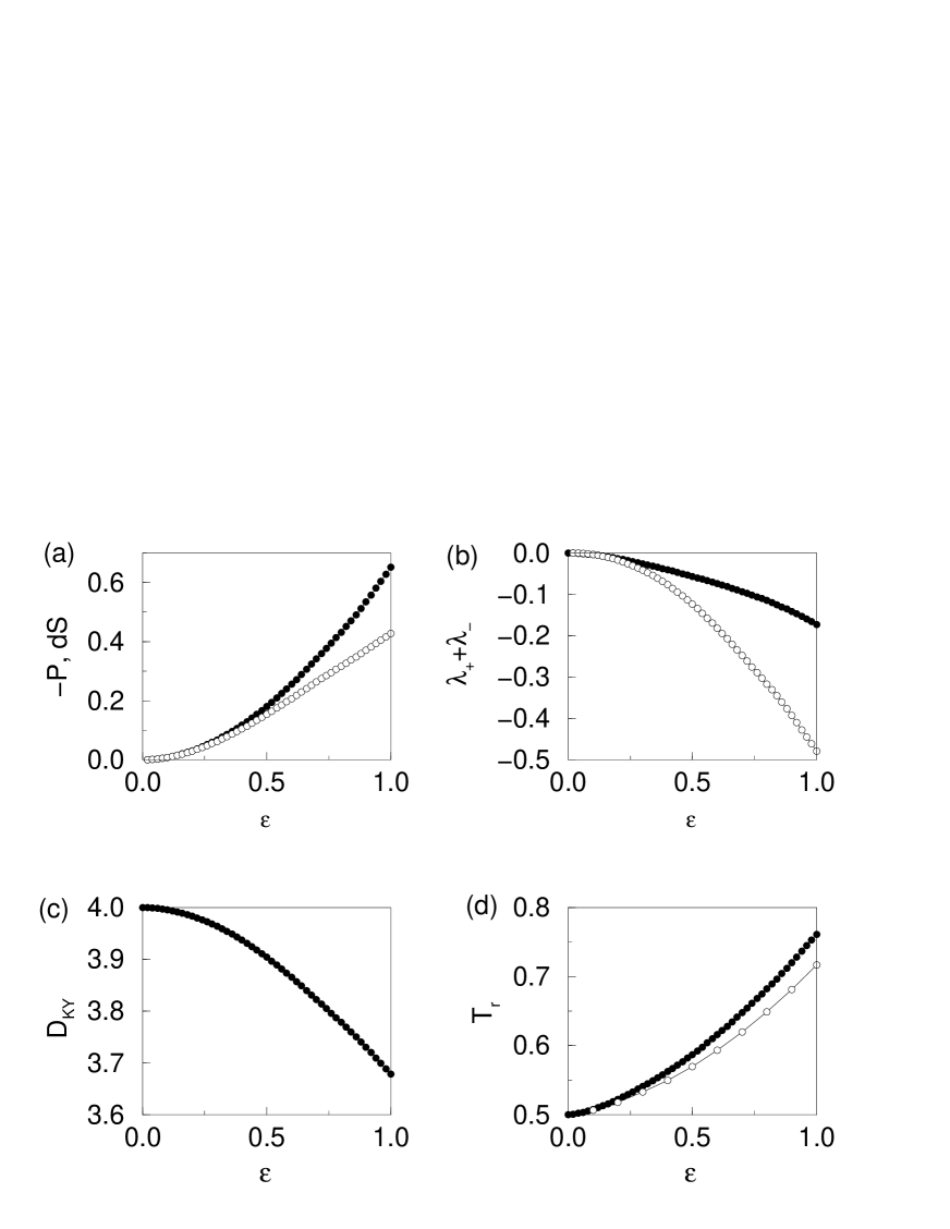
FIG. 4.: Field dependence of various important quantities in nonequilibrium: (a) black: phase space contraction rate $-P$, white: irreversible entropy production $dS$; (b) conjugate pairs of Lyapunov exponents, black: $\lambda_{1}+\lambda_{4}$, white: $\lambda_{2}+\lambda_{3}$; (c) Kaplan-Yorke dimension $D_{KY}$; (d) reservoir temperature $T_{r}$ (black) and its lower bound $T_{lr}$ (white).

FIG. 5.: Different quantities evaluated at the collision of a particle with the disk at field strength $\varepsilon_{x}=0.5$: (a) density at a collision $\varrho(\beta)$; (b) local stretching rate $\lambda_{c}(\beta)$, (c) reservoir temperature $T_{r}(\beta)$.

FIG. 6.: Probability density at the moment of a collision for (a) tangential velocity $v_{t}$ and (b) normal component $v_{n}$ at field strength $\varepsilon_{x}=0.5$; solid curve: density before collision, dashed curve: density after collision, long dashed curve: density in equilibrium.

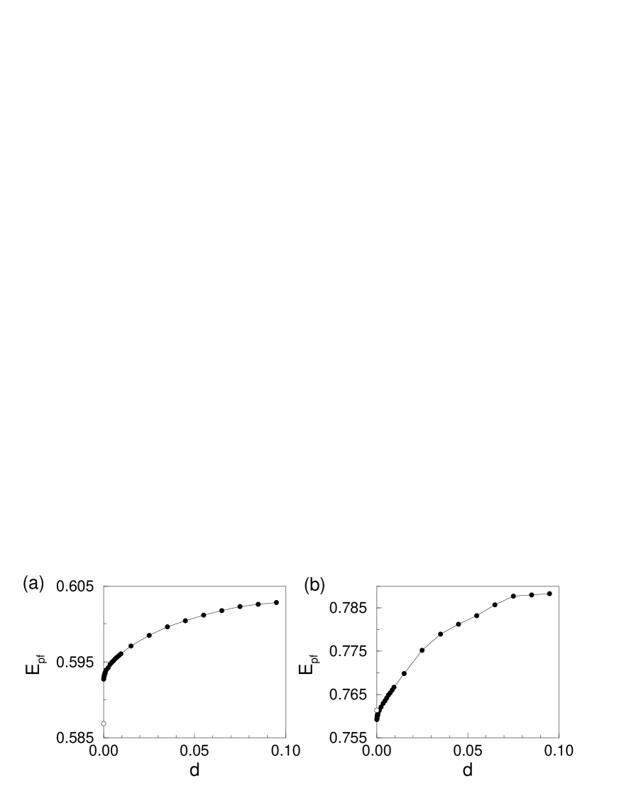
FIG. 7.: Profile of the full kinetic energy $E_{pf}$ of the particle in the bulk, black $E_{pf}$, white reservoir temperature $T_{r}$ (a) field strength $\varepsilon_{x}=0.5$, (b) $\varepsilon_{x}=1$.

REFERENCES

- [1] D. J. Evans and G. P. Morriss, Statistical Mechanics of Nonequilibrium Liquids (Academic Press, London, 1990).
- [2] W. G. Hoover, Computational Statistical Mechanics (Elsevier, Amsterdam, 1991).
- [3] G. P. Morriss and C. P. Dettmann, Chaos 8, 321 (1998).
- [4] R. Klages, K. Rateitschak, and G. Nicolis, Phys. Rev. Lett. 84, 4268 (2000).
- [5] W. G. Hoover, A. J. C. Ladd, and B. Moran, Phys. Rev. Lett. 48, 1818 (1982).
- [6] D. J. Evans, J. Chem. Phys. 78, 3297 (1983).
- [7] D. J. Evans et al., Phys. Rev. A 28, 1016 (1983).
- [8] S. Nosé, J. Chem. Phys. 81, 511 (1984).
- [9] W. G. Hoover, Phys. Rev. A 31, 1695 (1985).
- [10] D. J. Evans and B. L. Holian, Phys. Rev. A 83, 4069 (1985).
- [11] B. Moran and W. G. Hoover, J. Stat. Phys. 48, 709 (1987).
- [12] B. L. Holian, W. G. Hoover, and H. A. Posch, Phys. Rev. Lett. 59, 10 (1987).
- [13] W. G. Hoover, Phys. Rev. A 37, 252 (1988).
- [14] W. G. Hoover, Time Reversibility, Computer Simulation, and Chaos (World Scientific, Singapore, 1999).
- [15] W. G. Hoover and B. Moran, Phys. Rev. A 40, 5319 (1989).
- [16] G. P. Morriss, Phys. Lett. A 134, 307 (1989).
- [17] H. A. Posch and W. G. Hoover, Phys. Rev. A 38, 473 (1988).
- [18] N. L. Chernov, C. L. Eyink, J. L. Lebowitz, and Y. G. Sinai, Phys. Rev. Lett. 70, 2209 (1993).
- [19] N. L. Chernov, C. L. Eyink, J. L. Lebowitz, and Y. G. Sinai, Comm. Math. Phys. 154, 569 (1993).
- [20] D. J. Evans, E. G. D. Cohen, and G. P. Morris, Phys. Rev. A 42, 5990 (1990).
- [21] C. Dellago, L. Glatz, and H. A. Posch, Phys. Rev. E 52, 4817 (1995).
- [22] J. Lloyd, L. Rondoni, and G. P. Morriss, Phys. Rev. E 50, 3416 (1994).
- [23] J. Lloyd, M. Niemeyer, L. Rondoni, and G. P. Morriss, Chaos 5, 536 (1995).
- [24] C. P. Dettmann and G. P. Morriss, Phys. Rev. E 54, 4782 (1996).
- [25] K. Rateitschak, R. Klages, and W. G. Hoover, J. Stat. Phys. 101, 61 (2000).
- [26] C. P. Dettmann, in Hard ball systems and the Lorentz gas, Springer-Series ’Encyclopedia of mathematical sciences’, edited by D. Szasz (Springer, Berlin, 2000).
- [27] K. Rateitschak, R. Klages, and G. Nicolis, J. Stat. Phys. 99, 1339 (2000).
- [28] C. Wagner, R. Klages, and G. Nicolis, Phys. Rev. E 60, 1401 (1999).
- [29] C. Dellago, H. A. Posch, and W. G. Hoover, Phys. Rev. E 53, 1485 (1996).
- [30] C. Wagner, J. Stat. Phys. 98, 723 (2000).
- [31] H. Schuster, Deterministic Chaos, 2nd ed. (VCH Verlagsgesellschaft mbH, Weinheim, 1989).
- [32] J.-P. Eckmann and D. Ruelle, Rev. Mod. Phys. 57, 617 (1985).
- [33] G. Benettin, L. Galgani, A. Giorgili, and J.-M. Strelcyn, Meccanica 15, 9 (1980).
- [34] A. Wolf, J. B. Swift, H. L. Swinney, and J. A. Vastano, Physica D 16, 285 (1985).
- [35] C. Dellago and H. A. Posch, Phys. Rev. E 52, 2401 (1995).
- [36] P. Gaspard, Chaos, Scattering, and Statistical Mechanics (Cambridge University Press, Cambridge, 1998).
- [37] K. Rateitschak and R. Klages (unpublished).
- [38] This failure of the Gram-Schmidt orthonormalization was not detected in related calculations for a shear flow as thermostated by deterministic scattering [30]. We suspect that, because of the many elastic particle-particle collisions in the bulk, in this system it has quantitatively negligible consequences.
- [39] C. Dellago and W. G. Hoover, Phys. Lett. A 268, 330 (2000).
- [40] P.Gaspard, private communication.
- [41] One week CPU time was not sufficient to increase the quality of the results.
- [42] G. Morriss, C. Dettmann, and D. Isbister, Phys Rev E 54, 4748 (1996).
- [43] C. Dettmann, G. Morriss, and L. Rondoni, Phys Rev E 52, R5746 (1995).
- [44] H. A. Posch and W. G. Hoover, Phys. Rev. A 39, 2175 (1989).