Analytic solutions for nonlinear waves in coupled reacting systems

Abstract

We analyze a system of reacting elements harmonically coupled to nearest neighbors in the continuum limit. An analytic solution is found for traveling waves. The procedure is used to find oscillatory as well as solitary waves. A comparison is made between exact solutions and solutions of the piecewise linearized system, showing how the linearization affects the amplitude and frequency of the solutions.

I Introduction

Consider a lattice consisting of a reaction system at each site $n$, described by a site potential $V(u_{n})$ with $u$ a one dimensional field. Neighboring sites in the lattice interact through a potential $\phi(u)$. The equation of motion:

$$\frac{d^{2}u_{n}}{dt^{2}}=-\phi^{\prime}(u_{n}-u_{n-1})+\phi^{\prime}(u_{n+1}-u_{n})-V^{\prime}(u_{n}).$$ (1)

describes, for instance, the time evolution of the amplitude of an oscillator, the population of some ecological species, or the density of a chemical component of the system. If $\phi$ is quadratic, the continuous form of Eq. (1) is a wave equation augmented by an additive nonlinear term:

$$\frac{\partial^{2}u}{\partial t^{2}}=v^{2}\,\frac{\partial^{2}u}{\partial x^{2}}-V^{\prime}(u),$$ (2)

where $v$ is the speed of linear waves in the absence of the nonlinear potential $V$. The latter is determined by the details of the system under consideration. A choice of wide applicability is the logistic reaction term. Equation (2) is then:

$$\frac{\partial^{2}u}{\partial t^{2}}=v^{2}\,\frac{\partial^{2}u}{\partial x^{2}}+k\,u(1-u),$$ (3)

whose interest resides in its relevance to chemical and population dynamics, where the reaction term models an autocatalytical “malthusian” growth of $u$, with a saturation due to intraspecies competition. We have taken rescaled variables in Eq. (3) so that the carrying capacity of the medium is 1, in order to simplify the notation.

Equation (3) is very closely related to the so-called Fisher’s equation murray for reaction-diffusive systems, in which the left hand side of Eq. (3) is replaced by the first-order time derivative $\partial u/\partial t$. The two equations share the same nonlinear reaction term but, respectively, represent opposite limits of completely coherent (wave-like) and completely incoherent (diffusive) transport in the absence of the reaction term. Generalizations of Fisher’s equation that take into account finite correlation time effects in the transport term have been studied recently MHK ; ABK .

The logistic term $u(1-u)$ bears similarity to $\sin u$ between its zeros. Replacement of the former term by the latter makes Eq. (3) the sine-Gordon equation which describes, for example, the continuous limit of a chain of harmonically coupled pendulums dodd . The main difference between the two equations is the periodicity of $\sin u$ and, consequently, an infinite number of zeros (equilibria). The logistic term provides only two equilibria. Obviously, we expect low amplitude solutions of Eq. (3) to be qualitatively similar to sine-Gordon’s solutions, and large amplitude solutions (in particular solitary wave solutions connecting the two equilibria) to be quite different from the solitonic solutions of the sine-Gordon equation.

We analyze in this paper traveling wave solutions of Eqs. (3), which can be calculated exactly by analytical means. It is customary to analyze a piecewise linear simplification of a nonlinear system like Eq. (3), such as is done in Ref. MHK . Our analytic solution will provide us an opportunity to assess the validity of a piecewise linearization of the problem. Traveling waves of a related equation are analyzed in Section III.

II Traveling waves

We look for traveling-wave solutions of Eq. (3), moving in the direction of increasing $x$, by means of the ansatz: $u(x-ct)=U(z)$. In general $c$, the speed of the nonlinear waves, will be different from $v$, the speed of the linear waves dictated by the medium. The ordinary differential equation describing the shape of the wave is:

$$(c^{2}-v^{2})\,U^{\prime\prime}=kf(U)=-\,\frac{\partial V}{\partial U}.$$ (4)

A mechanical analogy involving a particle of mass $m=|c^{2}-v^{2}|$ is immediately available (see e.g. MHK ). Explicit solutions can be found by multiplying Eq. (4) by $U^{\prime}$ and integrating to find:

$$\frac{1}{2}(c^{2}-v^{2})U^{\prime 2}-E=\int kf(U)dU\equiv-V(U),$$ (5)

where $E$ is the “energy” of the particle, that depends on the initial conditions. Integrating once more:

$$z-z_{0}=\int_{U_{0}}^{U}\frac{dU^{\prime}}{\sqrt{\frac{2}{c^{2}-v^{2}}[E-V(U^{\prime})]}}.$$ (6)

This is an elliptic integral that can be solved exactly since the radicand is a cubic function of $U$. This is done in Section II.1.

Figure 1: The potentials of the mechanical analog of Eq. (4). The cases shown are $V$ and $\tilde{V}$, corresponding to faster than $v$ and slower than $v$ traveling waves respectively.

The potential of this mechanical system is $V(U)=k(U^{3}/3-U^{2}/2)$ if $c>v$, and $\tilde{V}(U)=-V(U)$ if $c<v$ (refer to Fig. 1 for a comparison). The potential $V$ has a maximum $V=0$ at $U=0$ and a minimum at $U=1$. Thus, if $c>v$, the system performs oscillations around $U=1$, with the amplitude $U$ always remaining positive, provided that the energy satisfies $-k/6<E<0$. If $E=0$ there is a solitary-wave solution with the shape of a traveling pulse, growing from $U=0$ to $U=1.5$ and back to $U=0$.

The potential $\tilde{V}$, instead, has a minimum at $U=0$ and a maximum at $U=1$. The system oscillates around $U=0$ if the energy is positive and smaller than a finite value ($0<E<k/6$), and a traveling trough if it is exactly this value. Since we are interested in situations where $u$ describes a density or a population, we will exclude these solutions that contain a negative amplitude in the present discussion. Nevertheless, they can be analyzed without difficulty in the same way.

II.1 General solutions

As we noted, $U(z)$ can be found exactly by performing the elliptic integral in Eq. (6). Note the following simplified form mathematica :

$$\int\frac{dU}{\sqrt{1-U^{3}+U^{2}}}=A{\cal F}\left(\arg\sin\sqrt{B+CU}|\gamma\right),$$ (7)

where ${\cal F}(\phi|\gamma)$ is the elliptic integral of the first kind, and $A$, $B$, $C$, and $\gamma$ are constants involving the roots of $1-U^{3}+U^{2}$. The constant $\gamma$ is termed the modulus of the elliptic integral, not to be confused with the parameter which is $m=\gamma^{2}$. (We are following the nomenclature of Ref. byrd , chapter 8.1, but denoting the modulus $\gamma$ instead of $k$ to avoid confusion with the reaction constant.) The relation between the elliptic integral ${\cal F}$ and the jacobian elliptic function $\,\mbox{sn}(z|\gamma)$ suggests that the solution of Eq. (4) is of the form:

$$U(z)=A+B\,\mbox{sn}^{2}(\beta z|\gamma),$$ (8)

where $A$, $B$, $\beta$ and $\gamma$ are constants, depending on the initial conditions, that remain to be determined. Differentiating Eq. (8) with respect to $z$, squaring and multiplying by $m/2$, we arrive at:

$$\frac{m}{2}U^{\prime 2} = -2m\beta B(U-A)$$ (9)

$$\times\left[1-\frac{1-\gamma}{B}(U-A)+\frac{\gamma}{B^{2}}(U-A)^{2}\right].$$

Equation (9) is the kinetic energy, that we can equate to $E-V(U)$, which in turn we can write in the form:

$$E-V(U) = E-\frac{k}{3}\,U^{3}+\frac{k}{2}\,U^{2}$$ (10)

$$= \frac{k}{3}\,(U-U_{1})(U-U_{2})(U-U_{3}),$$

where $U_{1}$, $U_{2}$ and $U_{3}$ are the zeroes of $E-V$, and depend on the initial conditions. By equating Eq. (10) and Eq. (9) we can express the unknowns $A$, $B$, $\beta$ and $\gamma$ as functions of $U_{1}$, $U_{2}$, $U_{3}$ and $k$. Because these expressions are intricate and do not add much to the analysis, we do not display them. However, one of the consequences of these expressions is the following dispersion relation, relating the speed of the nonlinear waves to system parameters:

$$c=\left[v^{2}+\frac{k}{12\beta}\left(\alpha+\sqrt{2\alpha^{2}-(U_{1}-U_{3})^{2}}\right)\right]^{1/2},$$ (11)

where $\alpha=-U_{1}+2U_{2}-U_{3}$.

Equation (6) can also be integrated numerically to yield $z(U)$ for a given value of the energy $E$. In Fig. 2 we show half-waves for several energies. The complete solutions are periodic functions of $z$, symmetric around their maxima, and we are plotting here only one half of a period. These solutions correspond to waves of progressively lower energy, smaller amplitude and, as can be seen, corresponding higher frequency. A grey line relating amplitude to period connects the half periods, and can be seen to converge to a value of the half period of $\sqrt{2}\pi\approx 4.44$, corresponding to the harmonic small oscillations. Waves of diverging period eventually become a traveling pulse, that we describe below.

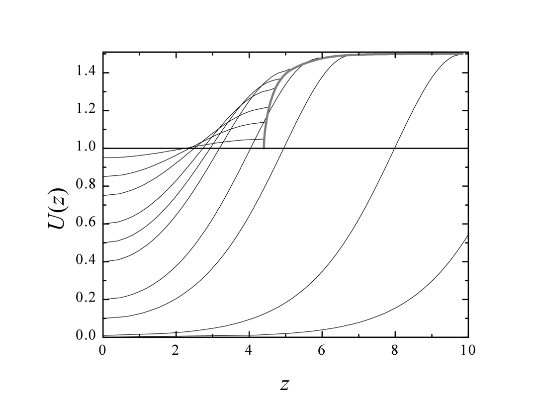
Figure 2: Half waves of the periodic solutions of different energy. Greater amplitude (and lower frequency) correspond to higher energy. The parameters are $k=1$, $m=2$.

II.2 Validity of piecewise linearization procedures

A piecewise linearization of Eq. (3) can be made, as in related models of reaction-diffusion processes (see for example mckean ; koga ; ohta for excitable systems, schat for an electrothermal instability, and the generalization of Fisher’s equation found in MHK ). Following MHK , the potential of the piecewise linear oscillator can be written as:

$$V(U)=\left\{\begin{array}[]{cl}\displaystyle-V_{0}kU^{2}/(2a),&\;\;\;U\leq a\\ \displaystyle V_{0}\frac{k}{b-a}(U^{2}/2-bU),&\;\;\;U\geq a.\end{array}\right.$$ (12)

with free parameters, $a$, $b$ and $V_{0}$, that can be adjusted to match the nonlinear one. The corresponding oscillator system is:

$$mU^{\prime\prime} = \frac{k}{ma}U\;\;\;\;\;\;(U\leq a),$$ (13)

$$mU^{\prime\prime} = -\frac{k}{m(b-a)}(U-b)\;\;\;\;(U\geq a),$$ (14)

whose solution can be found explicitly. Equations (13) and (14) describe harmonic oscillators, the first one with a positive restitutive force, so that the solution will be unstable (if $m>0$). If the initial condition $U_{0}$ is lower than $a$ and has zero velocity, the general solution is a smooth match (a continuous match of $U$ and $U^{\prime}$) of the solutions of both equations (13,14). If $U_{0}>a$ the solution is just that of (14).

We define natural frequencies: $\omega_{1}=\sqrt{k/m}$ and $\omega_{2}=\sqrt{k/[m(b-a)]}$. The solution to (13,14) is:

$$U(z)=\left\{\begin{array}[]{ll}\displaystyle U_{0}\cosh(\omega_{1}z),&\;\;\;U\leq a,\\ \displaystyle A\cos(\omega_{2}z)+B\sin(\omega_{2}z)+b,&\;\;\;U\geq a.\end{array}\right.$$ (15)

where $A$ and $B$ are found as a solution to the following linear system:

$$\begin{array}[]{rcrcl}\cos(\omega_{2}z_{a})\,A&+&\sin(\omega_{2}z_{a})\,B&=&a-b,\\ -\omega_{2}\sin(\omega_{2}z_{a})\,A&+&\omega_{2}\cos(\omega_{2}z_{a})\,B&=&U_{0}\omega_{1}\sinh(\omega_{1}z_{a}),\\ \end{array}$$ (16)

where $z_{a}$ is the time it takes the unstable solution to grow from $U_{0}$ to $a$, namely: $z_{a}=\omega_{1}^{-1}\arg\cosh(a/U_{0})$.

When the initial condition is greater than $a$, the solution is:

$$U(z)=(U_{0}-b)\cos(\omega_{2}z)+b,\;\;\;\;\;(U_{0}\geq a).$$ (17)

The two kinds of solutions (those of the nonlinear system and those of the piecewise linear) have the same qualitative shape. The piecewise linearization of the system is harmonic around the minimum at $U=b$, so there are harmonic oscillations of amplitude up to $b-a$ (oscillations of greater amplitude feel the nonlinearity at $U=a$). The frequency of these oscillations is $\omega_{lin}=\sqrt{k/[m(b-a)]}$. If $b=1$, $a=1/2$ and $V_{0}=1/4$ (to match the logistic case $U(1-U)$ as well as possible) then $\omega_{lin}=\sqrt{k/2m}$ which is $\sqrt{2}$ smaller than what is found for the nonlinear system.

This discrepancy can be seen in Fig. 3 where the relationship between the amplitude and the half period is shown, in a way similar to a dispersion relation. The nonlinear solution is shown as the full line. The piecewise linear solution that preserves the intensity of the nonlinearity is shown as the dashed line. It’s frequency at small amplitude overestimates the nonlinear one by a factor of $\sqrt{2}$.

Of course, the piecewise linear procedure can be adjusted to fit the parameter we want, such as the slope at $U=1$. In this case the frequency of oscillations is $\sqrt{k/m}$, but $f(a=1/2)=1/2$ instead of 1/4. This case is shown in Fig. 3 as the dotted line; it has the correct frequency at small amplitude. Both linearizations overestimate the amplitude of the nonlinear waves. Fig. 4 shows the three potentials. In can be seen that the amplitude of traveling waves of a certain energy will always be overestimated in the piecewise linear system.

Figure 3: Amplitude vs. half period of traveling wave solutions. Results are shown for the fully nonlinear system and for two piecewise linearizations: one that preserves the value $f(a)$ and one that preserves the slope of $f$ at $u=b$, as shown in the legend. The parameters are: $k=1$, $m=2$, $a=1/2$, $b=1$.

Figure 4: The potential of the mechanical analog of the fully nonlinear and the piecewise linear systems. The case shown corresponds to $c>v$.

II.3 Traveling pulse at $E=0$

When $E=0$ (and $c>v$) the solution is a traveling solitary pulse instead of a periodic wave. It corresponds to the case $\gamma=1$, when $\,\mbox{sn}(\phi|1)=\tanh(\phi)$, and it represents the trajectory of the particle leaving the maximum of $V$ at $U=0$ towards the right (see Fig. 4) and bouncing back to $U=0$ after reaching the maximum amplitude $U=1.5$. In this case, the integral (6) simplifies considerably, and the pulse can be written down explicitly as:

$$U(z)=\frac{3}{2}\left\{1-\left[\tanh\left(-\frac{z}{2}\sqrt{\frac{k}{c^{2}-v^{2}}}\right)\right]^{2}\right\}.$$ (18)

The speed of the pulse is related to its width. From the second moment of (18) we find the following expression for the velocity as a function of the parameters:

$$c(\sigma)=\sqrt{v^{2}+k\left(\sqrt{2}\pi^{2}\sigma^{2}\right)^{2/3}},$$ (19)

where $\sigma$ is the variance of (18). It can be seen that wider pulses move faster than narrow ones, much in the way that the less steep fronts are faster in Fisher’s equation murray .

This solitary wave solution is different from the kink-type soliton of the sine-Gordon equation, despite the similarity between the two equations. The potential in the sine-Gordon case is sinusoidal, allowing the state of the field $u$ to shift by amounts of $2\pi$ in a kink. In the present case the potential $V(u)$ continues growing as $u\rightarrow\infty$, and the state $u$ is forced back to $u=0$ after the excursion represented by the pulse (18).

III Front solutions for a related system

It is possible to approach our model of coupled reactors from another direction. Suppose that at each site of the lattice we have a system described by a first order equation of chemical or population dynamics:

$$\frac{du_{n}}{dt}=f(u_{n}).$$ (20)

So, if $f$ is logistic, the “force” (deriving (20) with respect to time) is the cubic $f^{\prime}(u)f(u)=k(1-2u)u(1-u)$ and the corresponding generalization of the wave equation is:

$$\frac{\partial^{2}u}{\partial t^{2}}=v^{2}\,\frac{\partial^{2}u}{\partial x^{2}}+ku(1-u)(1-2u).$$ (21)

Equation (21) is very similar to the $\phi^{4}$ equation of particle physics dodd . But in Eq. (21) the $u^{4}$ potential is inverted and it has as a consequence only one stable vacuum state instead of two.

Solutions of Eq. (21) are qualitatively similar to those of Eq. (3) around and near the equilibrium $u=0$. Solutions far from the equilibrium can be analyzed with the same methods as those of Eq. (3), since the integrals involved in (6) are also elliptic. In fact, Eq. (21) is similar to a Klein-Gordon $\phi^{4}$ model, but with an inverted potential. The solitary wave in this case is of the kink type, and it is straightforward to calculate its shape as $z(U)$:

$$z(U)=\sqrt{\frac{m}{2k}}\frac{U(1-U)\log{[(1-U)/U]}}{\sqrt{U^{4}/2-U^{3}+U^{2}/2}}.$$ (22)

This solution is a traveling front, connecting the hyperbolic points located at the two maxima of the potential, at $U=0$ and $U=1$. It represents the invasion of one of the states by the other. A kink from $U=0$ to $U=1$ as well as an “anti-kink” from $U=1$ to $U=0$ are possible, opening interesting possibilities of multiple interacting kinks, which will be analyzed elsewhere.

Oscillatory wave solutions are plotted in Fig. 5 for several initial conditions. Lower energies tend to accumulate to the kink solution (22), shown with a thicker line in grey.

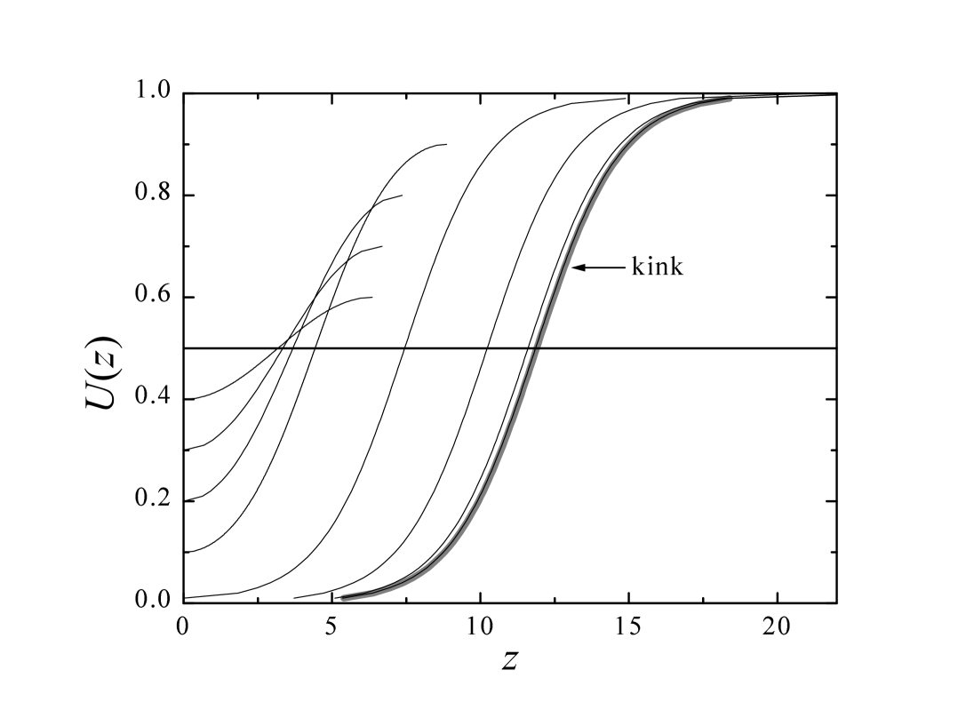
Figure 5: Half waves of the periodic solutions of Eq. (21) (thin black lines) and kink solution (22) (thick grey line). Different lines correspond to different negative energies of the mechanical analog. The kink is the solution with zero energy.

IV Conclusion

We have analyzed two systems of reacting elements harmonically coupled to first neighbors. The equation of motion in the continuous limit is, in each case, a wave equation with a nonlinear reaction term. The transport character in the systems is, thus, fully coherent, in contrast to a case such as that of Fisher’s equation murray , in which it is fully incoherent. Intermediate transport coherence has been analyzed recently MHK ; ABK through the incorporation of memory functions and it has been shown how the incoherent (Fisher) limit may be obtained for a memory with infinitely fast decay. The opposite limit wherein the memory is constant is Eq. (3) in the present paper, while a related system is Eq. (21). The latter represents a set of logistic systems, coupled harmonically. There is an interesting difference between its solutions and those of other extended reaction models. In Fisher’s reaction-diffusion equation, traveling front solutions of a single kind are found. In the generalized system studied by us elsewhere ABK , two kinds of fronts—a front and an “anti-front”—have been found, which however cannot coexist: each exists for a different set of system parameters. By contrast, in the purely wave-like system we have studied in the present paper, the coexistence of kinks and anti-kinks is certainly possible. This opens an interesting possibility of multiple interacting fronts.

- (1) J. D. Murray, Mathematical Biology, 2nd ed. (Springer, New York, 1993).
- (2) K. K. Manne, A. J. Hurd and V. M. Kenkre, Phys. Rev. E 61, 4177 (2000).
- (3) G. Abramson, A. R. Bishop and V. M. Kenkre, preprint nlin.PS/0107043.
- (4) R. K. Dodd et al., Solitons and Nonlinear Wave Equations (Academic Press, London, 1982).
- (5) Wolfram Research, Inc., Mathematica, version 4, (Wolfram Research, Inc., Champaign, IL, 1999).
- (6) P. F. Byrd and M. D. Friedman, Handbook of elliptic integrals for engineers and scientists, 2nd ed., (Springer-Verlag, Berlin, New York, 1971).
- (7) H. P. McKean, Adv. Math. 4, 209 (1970).
- (8) S. Koga and Y. Kuramoto, Progr. Theor. Phys. 63, 106 (1980).
- (9) T. Ohta, A. Ito and A. Tetsuke, Phys. Rev. A 42, 3225 (1990); T. Ohta, Progr. Theor. Phys. S. 99, 425 (1989); T. Ohta, M. Mimura and R. Kobayashi, Physica D 34, 115 (1989).
- (10) C. Schat and H. S. Wio, Physica A 180, 295 (1992).