Precision Measurements of Stretching and Compression in Fluid Mixing

The mixing of an impurity into a flowing fluid is an important process in many areas of science, including geophysical processes, chemical reactors, and microfluidic devices. In some cases, for example periodic flows, the concepts of nonlinear dynamics provide a deep theoretical basis for understanding mixing[1, 2, 3, 4, 5, 6]. Unfortunately, the building blocks of this theory, i.e. the fixed points and invariant manifolds of the associated Poincaré map, have remained inaccessible to direct experimental study, thus limiting the insight that could be obtained. Using precision measurements of tracer particle trajectories in a two-dimensional fluid flow producing chaotic mixing, we directly measure the time-dependent stretching and compression fields. These quantities, previously available only numerically, attain local maxima along lines coinciding with the stable and unstable manifolds, thus revealing the dynamical structures that control mixing. Contours or level sets of a passive impurity field are found to be aligned parallel to the lines of large compression (unstable manifolds) at each instant. This connection appears to persist as the onset of turbulence is approached.

The relationship between the velocity field of a fluid flow and the pattern formed by an impurity that it disperses can be intricate. Even simple time-periodic flows in two dimensions can produce chaotic mixing and complex distributions of material, in which nearby fluid elements diverge strongly from each other [1]. The fundamental processes involve a combination of repeated stretching and folding of fluid elements in combination with diffusion at small scales. However, to understand how the complex distributions of material actually arise, it is important to determine the nonlinear maps that connect the positions of fluid elements at different times, and to show how these maps separate nearby elements. This requires more precise and rapid measurement of flow fields than has been accomplished previously.

Our work depends on high resolution measurements of particle displacements in a two dimensional flow described later. Approximately 800 fluorescent latex particles ($120~{}\mu{m}$ in diameter) are suspended in the flow and followed by recording up to 15,000 512x512 pixel images at 10 Hz in a typical run, or 40-180 images per period. The centroid of each of the 12,000,000 particles in the sequence of images is found to a precision of about $40~{}\mu{m}$ (0.2 pixels). Particles found in sequential images are then combined into tracks. Since the flow studied here is time-periodic, we use conditional sampling, grouping together particle positions in all images at the same phase relative to the forcing. This process yields 100,000 precise particle positions at each phase, velocities accurate to a few percent, spatial resolution of 0.003 of the field of view, and time resolution of about 0.01 periods.

We rely on recent theoretical work in which stable and unstable manifolds are determined from finite-time velocity or displacement data[7, 8, 9, 10]. Specifically, from the measured velocity field, we determine the flow map $\vec{x}^{\,\prime}=\vec{\Phi}(\vec{x},t_{0},\Delta t),$ a function that specifies the destination vector $\vec{x}^{\,\prime}$ at time $t_{0}+\Delta t$ of any fluid particle starting from $\vec{x}$ at time $t_{0}$. (For $\Delta t$ equal to one period, $\vec{\Phi}$ becomes the Poincaré map of the flow.) The stretching and compression fields are then obtained from its gradients with excellent resolution. We identify the maximal stretching experienced by a fluid element as the square root of the largest eigenvalue of the right Cauchy-Green strain tensor, $C_{ij},$ at that location: $C_{ij}=(\partial\Phi_{k}/\partial x_{i})(\partial\Phi_{k}/\partial x_{j}),$ where summation is implied over the repeated index $k=1,2$. Similarly, the maximal compression at any location $\vec{x}$ is obtained as the stretching for the backward-time flow map $\vec{\Phi}(\vec{x},t_{0},-\Delta t).$ We note that the largest finite-time Lyapunov exponent is given by the logarithm of the stretching after division by $2\Delta t$. The stable and unstable manifolds should coincide with local maxima of the stretching and compression fields[9].

To extract the flow map and its gradients, we first measure particle velocities from trajectories using polynomial fitting. The velocities are then interpolated onto a grid to obtain the velocity as a function of space and phase. Numerical integration of hypothetical particle trajectories from these velocity fields produces flow maps with extremely high resolution. Although errors in measured particle positions grow exponentially in chaotic flows, the errors in the extracted invariant manifolds remain small, as we confirm experimentally.

The two-dimensional flow is produced by density stratification and time-periodic magnetic forcing[11]. A sinusoidal electric current through a thin conducting fluid layer placed above an array of permanent magnets generates a flow by means of Lorenz forces. The fluid of interest is a 1 mm thick non-conducting upper layer floating on the lower driven layer. The fluids are glycerol-water mixtures, with the lower layer also containing salt. Though miscible, the two layers remain distinct over the course of an experiment, and the flow stays essentially two-dimensional. The flow is a time-dependent vortex array, spatially disordered in the work described here. The flow is 15x15 cm, and all the figures in this paper show a central 10x10 cm region. Typical forcing frequencies are 10-200 mHz, and typical velocities are 0.05-1 cm/s. In some experiments, part of the upper layer contains fluorescein dye, whose emission in the visible under UV illumination is accurately proportional to the local concentration.

The general behavior of this system has been described elsewhere[11]. After an initial transient, the concentration field reaches a nearly steady state in which stretching and folding balance diffusion in such a way that the pattern recurs once per cycle of the forcing, except for a slow overall exponential decay of contrast. This striking process may be viewed in the supplementary animation available on-line[12].

There are two important control parameters. The Reynolds number $Re=UL/\nu$ (based on the mean magnet spacing $L=2$ cm, rms velocity $U$, and kinematic viscosity $\nu$) is typically between 10 and 200. The second parameter is the mean path length $p=UT/L$ in one forcing period $T$, which is typically in the range 0.5 to 10. Chaotic mixing is weak at the lower end of the ranges of $Re$ and $p$, where the unmixed elliptic regions are large, and mixing grows stronger as $Re$ and $p$ are increased. Both parameters are controlled by the forcing current, its frequency, and the fluid viscosity. The flow becomes non-periodic or weakly turbulent in the range $Re=100-150$, depending on $p$.

Figure 1 shows examples of one component of the velocity field for a run at $Re=45$ and $p=1$. Both components are available as a function of time, and an animation may be viewed on-line[12]. The two fields shown in Figure 1 are taken at equal time increments before and after the minimum of the magnitude of the velocity field. Because these are not identical (due to the non-zero $Re$), particles do not generally retrace their paths and chaotic mixing occurs, despite the time reversal symmetry of the forcing.

Studying mixing requires following fluid elements over extended times. Fig. 2 shows the particle displacements over one period, i.e. a Poincaré map. In these maps, lines are drawn from the measured initial to final particle positions, and pseudocolor is used to show the large and small displacements. Points at which there is no net motion over a full period are called fixed points. Both elliptic and hyperbolic fixed points may be seen. Figure 2(B) shows a 4X enlargement of part of the Poincaré map. The fixed points in this map have been marked. The hyperbolic fixed points are saddles, with one axis of approach (stable manifolds) and one axis of departure (unstable manifolds). In the remainder of this paper we show how these fixed points and their stable and unstable manifolds are related to the stretching and compression fields and to the concentration field of an impurity such as a dye.

The key to this analysis is to compute the compression and stretching fields. We begin (Fig. 3A) with an example of the compression field, which is a measure of local convergence. It consists of large values along relatively sharp lines, and much smaller values between them. Its determination requires the selection of a time interval $\Delta t$ for the map; here it is 3 periods. Much smaller values result in broader structures, because less time is then available for compression to occur. Much larger values of $\Delta t$ cause the flow map to develop structures that are smaller than the spatial resolution. The optimum choice is a balance of competing factors, but there is a fairly wide acceptable range between 1 and 5 periods. An animation showing how the compression field depends on $\Delta t$ is available on-line[12].

The dye concentration field is shown at the same phase (or time) in Fig. 3B. In Fig. 3C, we superimpose the compression field on the dye image. The dye visualization and particle tracking data are measured in separate experiments at the same parameters. We observe that the level sets (contour lines) of the concentration field line up with the lines of strong compression. Furthermore, we find this to be the case at each instant or phase (see the on-line animation[12]). Several authors have described similar asymptotic alignment properties for numerically computed two-dimensional time-periodic flows[3, 6, 13, 14].

Now we discuss the correspondence between the lines of stretching and compression, and the fixed points of the Poincaré map, as shown in Fig. 4. Here we show the stretching field (blue) in addition to the compression field (red). One can see that many of the points where the two sets of lines cross correspond to hyperbolic fixed points of the flow field. The lines of maximum stretching and compression label the stable and unstable manifolds of these fixed points[9]. Thus, we have the following correspondence between the various objects: large stretching $\leftrightarrow$ stable manifolds; large compression $\leftrightarrow$ unstable manifolds. This demonstrated ability to measure the locations of both the stable and unstable manifolds as a function of time in complicated experimental flows opens new possibilities to apply the insights of lobe dynamics[3, 4] to practical mixing flows. An animation[12] shows the superimposed stretching and compression fields, which form homoclinic and heteroclinic tangles of invariant manifolds.

We have also carried out this analysis at higher values of $Re$ and $p$, as shown in Fig. 5. Under these conditions, the fixed points themselves are much harder to determine, because the stretching and compression are then much greater. Our measurements do not reveal any regular islands under these conditions. However, the concentration field is still organized by the invariant manifolds, with contours of constant concentration aligning with the lines of large compression. This is particularly dramatic in a time-dependent animation[12].

It is of interest to consider how the dynamics of mixing is affected when the flow becomes weakly turbulent, i.e. nonperiodic. Theoretical and numerical work indicates that the stretching and compression fields continue to form well defined lines that organize mixing[8]. To explore this issue experimentally, we analyzed the stretching in a flow at $Re=115$, $p=5$. Though $Re$ is only slightly elevated compared to the flow in Fig. 5, the velocity field has bifurcated to a period doubled state that repeats every second forcing period. We find that the lines of the stretching and compression fields remain nearly unchanged and continue to align with the dye pattern at each instant. This suggests that the same will be true even in non-periodic flows, and that there will therefore be a close correspondence between the kinematics of chaotic and turbulent mixing.

We have shown that lines of maximal stretching and compression corresponding to invariant manifolds of flow maps can be determined from precise experimental measurements of particle trajectories. These special material lines, which emerge from hyperbolic fixed points of the flow map, organize the evolution of inhomogeneous impurities in the flow. We find that the dye contour lines and the lines of maximal compression are locally parallel. This is true at each instant in the time-dependent flow, and continues to be the case at higher $Re$ where the fixed points themselves are hard to determine.

It is striking to realize that the intricate dynamical processes revealed here underlie mixing in many natural and artificial flows. It would be particularly interesting to predict the rate of homogenization of an impurity from the stretching and compression fields. Theoretical models show how this may be accomplished by extending this work to measure stretching over longer times than is currently feasible[15]. Eventually it may prove possible to utilize measurements such as these to control mixing by modifying the behavior in regions that are particularly active such as the region where the lines are dense in Fig. 4.

I Acknowledgements

We appreciate helpful discussions with B. Eckhardt and I. Mezic.

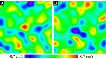
FIG. 1.: Maps of one component of the velocity field in the 2D flow measured at two instants equidistant from the instant of minimum flow ($p=1$, $Re=45$). The fact that one image is not the negative of the other is an example of the breaking of time reversal symmetry required for chaotic mixing.

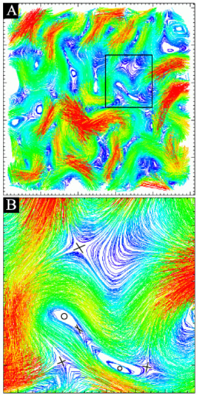
FIG. 2.: Poincaré map of the flow at one phase of the forcing ($p=1$, $Re=45$). Lines connect the experimentally measured initial coordinates of each particle with its coordinates one period later, with blue and red designating small and large displacements respectively. (A) Complete field of view. (B) A close-up of the region in the box in (A), showing two elliptic fixed points (circles), four hyperbolic fixed points (crosses), and the trajectories near them. The hyperbolic point between the two eliptic points is not fully resolved, but is clearly revealed by the manifolds in Fig. 4.

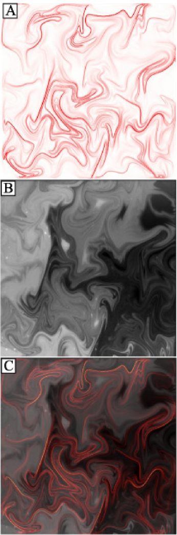
FIG. 3.: (A) Compression field calculated from trajectories obtained by integration of the measured velocity field. (B) Corresponding dye image showing the concentration after about 30 periods but at the same phase as in (A). (C) Superposition of the compression field with the corresponding dye image; the contour lines of the concentration field are aligned with the lines of large compression. This is from the same flow at the same phase as Fig. 2.

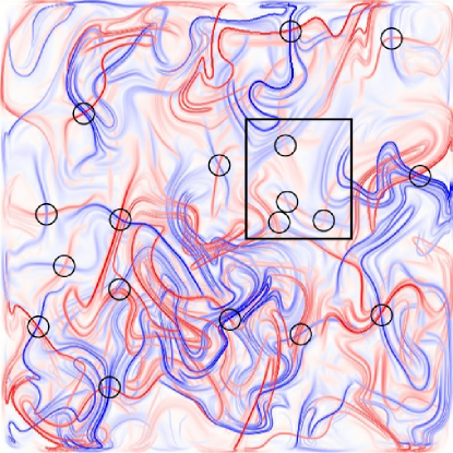
FIG. 4.: Lines of the stretching field (blue) and compression field (red), with some of the hyperbolic fixed points of the flow map marked by circles. Conditions match Figs. 2 and 3. The lines are respectively the stable and unstable manifolds of the fixed points of the Poincaré map. The box marks the region which is shown in Fig. 2(B). Note that some of the fixed points have only very weak stretching and compression lines associated with them. An online animation[12] shows the time dependence of the manifolds, which allows much greater insight into the dynamics of the mixing process.

FIG. 5.: Superposition of the compression field with a dye image at $Re=100$ and $p=5$. The pattern here resembles an array of random vortices, and the compression field lines are again found to align with the concentration field at each instant.

REFERENCES

- [1] H. Aref, Stirring by Chaotic Advection. J. Fluid Mech. 143, 1 (1984).
- [2] J. Ottino, The Kinematics of Mixing, Stretching, and Chaos, Cambridge University Press, Cambridge (1989).
- [3] V. Rom-Kedar, A. Leonard, and S. Wiggins, An analytical study of transport, mixing and chaos in an unsteady vortical flow. J. Fluid Mech. 214, 347 (1990).
- [4] V. Rom-Kedar, Homoclinic tangles-classification and applications. Nonlinearity 7, 441 (1994).
- [5] D. Beigie, A. Leonard, and S. Wiggins, Invariant manifold templates for chaotic advection. Chaos, Solitons, and Fractals 4, 749 (1994).
- [6] M. Giona, A. Adrover, F. Muzzio, S. Cerbelli, & M. Alvarez, The geometry of mixing in time-periodic chaotic flows. Physica D 132, 298 (1999).
- [7] P. D. Miller, C. K. R. T. Jones, A. M. Rogerson, and L. J. Pratt, Quantifying transport in numerically generated velocity fields. Physica D 110, 105 (1997).
- [8] G. Haller and G. Yuan, Lagrangian coherent structures and mixing in two-dimensional turbulence. Physica D 147, 352 (2000).
- [9] G. Haller, Distinguished material surfaces and coherent structures in three-dimensional fluid flows. Physica D 149, 248 (2001).
- [10] C. Coulliette and S. Wiggins, Intergyre transport in a wind-driven, quasigeostrophic double gyre: An application of lobe dynamics. Nonlin. Proc. Geophys. 8, 69 (2001).
- [11] D. Rothstein, E. Henry, & J. P. Gollub, Persistent patterns in transient chaotic fluid mixing. Nature 401, 770 (1999).
- [12] http://www.haverford.edu/physics-astro/Gollub/stretchlines/
- [13] F. Muzzio, P. Swanson, and J. Ottino, The statistics of stretching and stirring in chaotic flows. Phys. Fluids A 3, 822 (1991).
- [14] A. Péntek, T. Tél, and Z. Toroczkai, Chaotic advection in the velocity field of leapfrogging vortex pairs. J. Phys. A 28, 2191 (1995).
- [15] T. Antonsen, Z. Fan, E. Ott, and E. Garcia-Lopez, The role of chaotic orbits in the determination of power spectra of passive scalars. Phys. Fluids 8, 3094-3104 (1996).