In–out intermittency in PDE and ODE models

Abstract

We find concrete evidence for a recently discovered form of intermittency, referred to as in–out intermittency, in both PDE and ODE models of mean field dynamos. This type of intermittency (introduced in [4]) occurs in systems with invariant submanifolds and, as opposed to on–off intermittency which can also occur in skew product systems, it requires an absence of skew product structure. By this we mean that the dynamics on the attractor intermittent to the invariant manifold cannot be expressed simply as the dynamics on the invariant subspace forcing the transverse dynamics; the transverse dynamics will alter that tangential to the invariant subspace when one is far enough away from the invariant manifold.

Since general systems with invariant submanifolds are not likely to have skew product structure, this type of behaviour may be of physical relevance in a variety of dynamical settings.

The models employed here to demonstrate in–out intermittency are axisymmetric mean–field dynamo models which are often used to study the observed large scale magnetic variability in the Sun and solar-type stars. The occurrence of this type of intermittency in such models may be of interest in understanding some aspects of such variabilities.

Dynamical systems that possess symmetries (and hence invariant submanifolds embedded in their state spaces) are of interest in a variety of settings. In many simplified models such dynamical systems have skew product structure. For an ODE model, if $(x,y)$ parameterizes a phase space with an invariant manifold $y=0$, we say the system has skew product structure if $\dot{x}=f(x)$ and $\dot{y}=g(x,y)$, namely if the dynamics of $x$ is independent of $y$. A great deal of effort has gone into the study of such skew product systems with invariant manifolds, and these have thrown up a number of new and interesting phenomena.

In general, however, one would expect dynamical systems not to have skew product structure unless extra structure is present (for example if the transverse dynamics is always forced by the tangential dynamics). In the absence of such extra structure it is therefore interesting to see what new types of dynamics can appear in systems with invariant submanifolds. One such novel type of dynamical behaviour, in–out intermittency, is discussed and analysed in detail in [4] using a simple two-dimensional mapping. An important feature of this type of intermittency is that, as opposed to on–off intermittency, it requires the absence of a skew product structure.

In this paper we find concrete evidence for the occurrence of in–out intermittency in both PDE and ODE models both in terms of phase–space and also statistically. The models considered are examples of axisymmetric mean–field dynamo models which are often used in order to study the observed large scale magnetic variability in the Sun and solar-type stars. In addition to providing examples of in–out intermittency in PDE models, the occurrence of this type of intermittency in such models may be of interest in understanding some aspects of solar and stellar variabilities.

I Introduction

Many systems of physical interest possess symmetries which in turn induce invariant submanifolds in their state spaces. A great deal of effort has gone into the study of the dynamics and intermittent behaviour of such systems near their invariant submanifolds (see e.g. [1]). A class of dynamical systems with invariant submanifolds have been shown to be capable of producing a number of novel modes of behaviour, including on–off intermittency, which occurs as the result of an instability of an attractor in an invariant submanifold [1]. It manifests itself as an attractor whose trajectories get arbitrarily close to an attractor for the system in the invariant submanifold while intermittently making large deviations away. It can be modelled by a biased random walk of the logarithmic distance from the invariant submanifold [1].

Since the linearised behaviour near an invariant submanifold has a natural skew product structure (i.e. the linearised dynamics transverse to the invariant submanifold is forced by the dynamics within the submanifold) many such studies have tended to concentrate on systems that are of skew product type for simplicity, although it should be stated that on-off intermittency can be found in systems that do not have skew product structure.

Moreover, bifurcation problems in such settings have tended to concentrate on normal parameters, i.e. parameters that vary the global dynamics without changing the dynamics within an invariant submanifold. In general, dynamical systems are not skew products over the dynamics within any invariant subspace, and moreover they do not possess normal parameters[2].

The authors [3, 4] have recently shown that dropping these assumptions can lead to the presence of a number of novel types of dynamical behaviour, including a new type of intermittency, referred to as in–out intermittency. The presence of this type of intermittency has also been found in different distinct nonlinear dynamical systems [4, 5]. Furthermore, there have been interesting developments concerning the study of other phenomena – e.g. riddling – in these more general settings [6].

To characterise in–out intermittency, it is best to contrast it with on–off intermittency, as they both can occur in systems with invariant submanifolds. To begin with, it is useful to bear in mind that even though on–off intermittency can occur in non–skew product settings, all its necessary ingredients can be satisfied in skew product settings. In–out intermittency, on the other hand, requires the absence of skew product structure for its existence.

Briefly, we say that an attractor $A$ exhibits in–out intermittency to the invariant submanifold $M_{I}$, if the following are true [4]:

1. The intersection $A_{0}=A\cap M_{I}$ is not necessarily a minimal attractor, i.e. there can be proper subsets of $A_{0}$ that are attractors (for on–off intermittency $A_{0}$ is assumed to be minimal). This means that there can be different invariant sets in $A_{0}$ associated with attraction and repulsion transverse to $A_{0}$, hence the name in–out. These growing and decaying phases come about through different mechanisms within $M_{I}$. If the system has a skew–product structure, in–out intermittency reduces to on–off intermittency [4]. Fig. 1 shows a schematic representation of a typical trajectory for an in–out process near $M_{I}$.

   

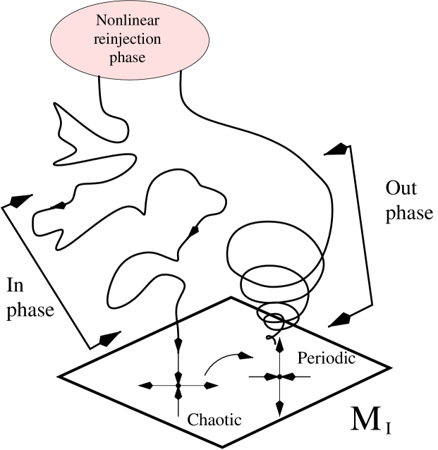
   FIG. 1.: Typical trajectory of an in–out intermittent solution close to the invariant submanifold $M_{I}$, with the two components, the “in” phase and the “out” phase. In the invariant submanifold $M_{I}$ we may have two or more invariant sets, one of which is transversely stable and chaotic but non–attracting in $M_{I}$ and another which is transversely unstable and is a periodic attractor in $M_{I}$. The injection mechanism, the “in” phase, is quite irregular and can be modelled by a random walk towards $M_{I}$, while the expelling mechanism, the “out” phase, can be modelled by a growing exponential spiral away from $M_{I}$. Note that the invariant sets in $M_{I}$ are represented as points only for clarity.

2. The minimal attractors in the invariant submanifold are not necessarily chaotic (as for on-off intermittency); they are very frequently periodic or equilibria. Furthermore, the trajectory remains close to one of these attractors during the moving away or “out” phases, with the important consequence that during these “out” phases the trajectory can shadow a periodic orbit, for example, while drifting away from $M_{I}$ at an exponential rate [4] (see also [7]).

3. The asymptotic scaling of the probability distribution of the duration of laminar phases in the in–out case can have two contributions:

   $$P_{n}\sim\overbrace{\underbrace{\alpha n^{-3/2}e^{(-\beta n)}}_{\rm on-off}+\gamma e^{(-\delta n)}}^{\rm in-out}=I_{1}+I_{2},$$ (1)

   where $\alpha>0$, $\delta>\beta>0$ and $\gamma>0$ are positive real constants depending on the bias of the random walk modelling the “in” phase and the probability of leaking into the deterministic “out” phase (see [4] for details). The term $I_{1}$ corresponds to biased on–off intermittency, while the extra term $I_{2}$ can cause an identifiable shoulder to develop at large laminar sizes $n$ which can help to statistically distinguish in–out from on–off intermittency.

The authors in [4] were motivated by a numerical exploration of a two dimensional map and explored the statistics by means of a Markov chain model. Our aims in this paper are twofold. Firstly, we demonstrate the occurrence of in–out intermittency in dynamical systems generated by ordinary differential equations (ODE) as well as by partial differential equations (PDE). The latter are especially of interest, since they are in principle infinite dimensional and also because few examples of intermittent behaviour and their scalings have been shown concretely to occur in such models (see e.g. [8]). Secondly, by choosing as our models the mean–field dynamo models [9], the occurrence of this type of intermittency could be of interest in understanding certain features of solar and stellar variability, and in particular we expect that due to its generic features, it may well appear in more detailed and accurate models of solar and stellar variability.

II In–out intermittency in Mean–Field dynamo models

Mean-field dynamo models have been employed extensively in order to study various aspects of the dynamics of solar, stellar and galactic dynamos (e.g. [10, 11]). Their rather idealised nature has been criticized by a number of authors (see e.g. [12]). However, such models are thought to capture some of the essential physics of the turbulent processes and reproduce many important dynamical and statistical features of the full three dimensional magneto-hydrodynamical models (see e.g. [13] and also [14]).

The standard mean–field dynamo equation is given by

$$\frac{\partial{\bf B}}{\partial t}=\nabla\times\left({\bf u}\times{\bf B}+\alpha{\bf B}-\eta_{t}\nabla\times{\bf B}\right),$$ (2)

where ${\bf B}$ and ${\bf u}$ are the mean magnetic field and mean velocity respectively and the turbulent magnetic diffusivity $\eta_{t}$ and the coefficient $\alpha$ arise from the correlation of small scale turbulent velocities and magnetic fields [9].

In axisymmetric geometry, equation (2) is solved by splitting the magnetic field into poloidal and toroidal components, ${\bf B}={\bf B_{p}}+{\bf B_{\phi}}$, and expressing these components in terms of scalar field functions

$${\bf B_{p}}={\bf\nabla}\times A(r,\theta,t){\bf\hat{\phi}},~{}~{}{\bf B}_{\phi}=B(r,\theta,t){\bf\hat{\phi}},$$

in spherical polar coordinates $(r,\theta,\phi)$. Equation (2) can then be expressed in terms of equations for the scalars $A$ and $B$,

$$\frac{\partial A}{\partial t} = \alpha B+\eta_{t}\left(\nabla^{2}-\frac{1}{r^{2}\sin^{2}\theta}\right)A,$$ (3)

$$\frac{\partial B}{\partial t} = r\sin\theta({\bf\nabla}\times A{\bf\hat{\phi}})\cdot{\bf\nabla}\omega$$ (7)

$$-\frac{1}{r\sin\theta}{\bf\nabla}\alpha\cdot{\bf\nabla}(Ar\sin\theta)$$

$$-\alpha\left(\nabla^{2}-\frac{1}{r^{2}\sin^{2}\theta}\right)A$$

$$+\eta_{t}\left(\nabla^{2}-\frac{1}{r^{2}\sin^{2}\theta}\right)B,$$

where ${\bf\nabla}\cdot A=0$ and we consider a purely rotational velocity ${\bf u}=\omega_{0}r^{2}\sin\theta\hat{\phi}$. Nondimensionalisation of these equations in terms of a length $R$ and a time $R^{2}/\eta_{t}$ produces the convective and rotational magnetic Reynolds numbers $C_{\alpha}=\alpha_{0}R/\eta_{t}$ and $C_{\omega}=\omega_{0}R^{2}/\eta_{t}$, where $\alpha_{0}$ and $\omega_{0}$ are typical values of $\alpha$ and $|\omega|$.

Solutions to these equations are often considered in the $\alpha\omega$ limit where the terms in $\alpha$ can be ignored in the equation for $B$, giving a single dynamo parameter $D=C_{\alpha}C_{\omega}$ on rescaling. This reflects the fact that, in stellar convective zones, rotational shear produces toroidal flux much more effectively than the processes represented by the $\alpha$ terms, whilst in the full equations (the so called $\alpha^{2}\omega$ limit) we retain both $C_{\alpha}$ and $C_{\omega}$ as two control parameters.

The equation (2) gives a kinematic dynamo, since the velocity field ${\bf u}$ is prescribed. As this equation stands there is no mechanism to limit the growth of the magnetic field a nonlinear saturation mechanism is usually supplied by making $\alpha$ depend on ${\bf B}$. This can be done by supplying a closed functional form representing a fixed approximation of the nonlinear effect (c.f. [15, 16]), or more dynamically, by supplying an auxiliary equation for $\alpha$ (c.f. [17] and references therein).

In the following we consider two cases arising from two separate studies [3, 16]: the above PDE model in the $\alpha^{2}\omega$ limit with two different algebraic forms for $\alpha(\bf{B})$ (c.f. [15, 16] and Figs. 5 and 6 captions) as well as a finite order truncation of it in the $\alpha\omega$ limit but with a time dependent form of the $\alpha$ effect in one spatial dimension (this can be obtained by averaging (2) over $r$) and using a spectral expansion [3]. This ODE model possesses a second (alongside $D$) control parameter, the magnetic Prandtl number $\nu=\nu_{t}/\eta_{t}$, where $\nu_{t}$ is the turbulent kinematic viscosity, which arises from the time dependent equation for $\alpha$. This model is given by

$$\frac{dA_{i}}{dt} = -i^{2}A_{i}+\frac{D}{2}(B_{i-1}+B_{i+1})$$ (9)

$$+\sum_{j=1}^{N}\sum_{k=1}^{N}F_{ijk}B_{j}C_{k},$$

$$\frac{dB_{i}}{dt} = -i^{2}B_{i}+\sum_{j=1}^{N}G_{ij}A_{j},$$ (10)

$$\frac{dC_{i}}{dt} = -\nu i^{2}C_{i}-\sum_{j=1}^{N}\sum_{k=1}^{N}H_{ijk}A_{j}B_{k},$$ (11)

where $A_{i}$, $B_{i}$ and $C_{i}$ are spatially independent coefficients of the spectral expansions of the scalar fields $A$, $B$ and $\alpha$ respectively, $F$, $H$ and $G$ are coefficients expressible in terms of $i,j$ and $k$, $N$ is the truncation order and $D$ and $\nu$ are the parameters defined above. The detailed derivation of these equations together with a phenomenological study of their dynamics is given in [3].

We note that the main ingredients necessary for the occurrence of in–out intermittency are present in both these models. Both are axisymmetric and possess invariant submanifolds. More precisely, the truncated model (9) with $N$=4 is a 12–dimensional system of ODEs with two 6–dimensional symmetric and antisymmetric invariant submanifolds given by

$$M_{S}=\{0,B_{1},0,A_{2},0,C_{2},0,B_{3},0,A_{4},0,C_{4}\},$$ (12)

$$M_{A}=\{A_{1},0,0,0,B_{2},C_{2},A_{3},0,0,0,B_{4},C_{4}\},$$ (13)

respectively. Similarly the PDE model (3) possesses two invariant submanifolds, the antisymmetric and symmetric invariant submanifolds which are given by

$${\rm M}_{A}\ :\ A(\theta)=A(-\theta),\quad B(\theta)=-B(-\theta),$$ (14)

$${\rm M}_{S}\ :\ A(\theta)=A(-\theta),\quad B(\theta)=B(-\theta),$$ (15)

respectively, where $\theta$ is the latitude.

If one separates the poloidal and toroidal scalar field components into symmetric and antisymmetric parts then the dynamic evolution for the symmetric (antisymmetric) components has contributions from antisymmetric (symmetric) counterparts. This means that these equations are of non–skew product type. For the ODE system (9) this can be readily seen by noting that the evolution equation for each component in $M_{S}$ ($M_{A}$) contains components from $M_{A}$ ($M_{S}$). For the PDE models, we first note that ${\bf u}$ in equation (2) is not dynamical: it is prescribed and therefore can be viewed as a part of the initial conditions. The non-skew product nature of the PDE models follows in a similar way to the ODE models, bearing in mind the form of the equation (2) and those of the invariant submanifolds (14) and (15).

Finally the control parameters $D$ and $\nu$ appearing in the ODE model (9) are generically non–normal as they enter the equations for $A_{i}$ and $C_{i}$ for all $i$. Similarly this is also true for the control parameters $C_{\alpha}$ and $C_{\omega}$ in the case of the nondimensionalised version of the PDE equations (3).

In this way, both models possess all the necessary ingredients for the occurrence of in–out intermittency.

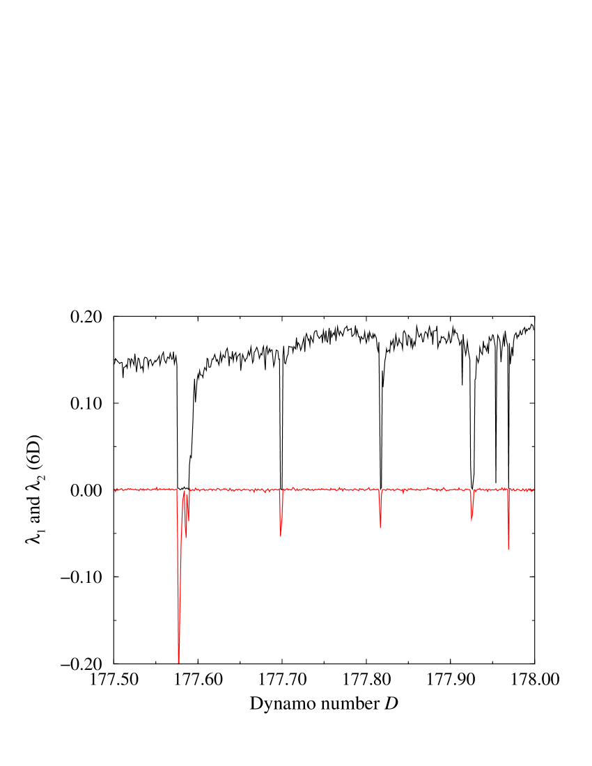
FIG. 2.: First and second Lyapunov exponents for the attractor of the ODE model (9) restricted to $M_{A}$ with $N$=4 and $\nu=0.47$, clearly showing the presence of windows of periodicity. Note that there is always one null Lyapunov exponent due to the system of equations (9) being autonomous.

Given that the ODE models are more transparent, we first demonstrate the presence of in–out intermittency in the truncated system (9) with $N$=4. For this model, in–out intermittency occurs for parameter values for which the system of equations (9) restricted to $M_{A}$ is within a window of periodicity (c.f. [18]). Fig. 2 depicts the presence of such windows for the ODE model (9). The presence of such windows is supported by a conjecture of Barreto et al. [18], according to which for chaotic systems with $k$ positive Lyapunov exponents and $m$ control parameters, with $m\geq k$, there is a dense set of nearby parameter values at which the attractors are periodic. This implies that for our system (9), for each parameter value at which there is a chaotic attractor in $M_{A}$ there are parameter windows arbitrarily close for which the attractor is periodic.

Fig. 3 shows an example of in–out intermittency in this system at parameter values $D=177.700196$ and $\nu=0.47$. We note that even though the interval reported here over which in–out occurs is small, nevertheless there are likely to be other intervals (according to the conjecture of Barreto et al., possibly an infinite number of them) over which this happens.

The top panel shows the periodic orbit in the antisymmetric invariant submanifold, $M_{A}$, which the projection of the trajectory of the full system shadows clearly (second panel). This shadowing or intermittent periodic locking of the tangential variables occurs within the laminar phases (third panel) where there is a simultaneous exponential growth (hence the name “out” phase) of the amplitudes of the transverse variables through several orders of magnitude (bottom panel). This last panel also shows the “in” phases, which can be modelled as a biased random walk taking the trajectory into the invariant submanifold.

FIG. 3.: In–out intermittency in the ODE model (9) with $N$=4 and parameter values $D=177.700196$ and $\nu=0.47$. The energy and parity are given by $E=E^{A}+E^{S}$ and $P=(E^{S}-E^{A})/E$ respectively, where $E^{A}$ and $E^{S}$ are the antisymmetric and symmetric parts of the magnetic field energy with respect to the equator (“antisymmetric” ($P=-1$) and “symmetric” ($P=+1$)). The top panel shows the evolution of an initial condition in $M_{A}$ and the other panels a nearby initial condition not in $M_{A}$. In these panels, we have taken a Poincaré section at $A_{1}$=0 for clarity and comparison.

FIG. 4.: Scaling of the probability distribution of the duration of laminar phases for the twelve–dimensional ODE truncated model (9) for the case considered in Fig. 3, using a time step $\tau=10^{-2}n$. The shoulder at large laminar phases (which identifies the influence of $I_{2}$ and is a characteristic of in–out intermittency) is easily discerned.

To substantiate this further, we also calculated the scaling of the probability distribution of the duration of laminar phases and this is shown in Fig. 4. This is compatible with the predicted scaling (1), possessing both a $n^{-3/2}$ section, at small laminar phase sizes, as well as a noticeable shoulder at higher laminar phase sizes, the latter being a distinctive signature of the in-out intermittency.

FIG. 5.: In–out intermittency in the axisymmetric PDE mean–field dynamo model (3). The parameters used were $r_{0}=0.4$, $C_{\alpha}=1.942$, $C_{\omega}=-10^{5}$, $f=0.0$, with the usual algebraic form of $\alpha=\alpha_{0}/(1+{\bf B}^{2})$ (see [16] for details of the parameters). To visually enhance the periodic locking we have time sampled the series in the two upper panels.

FIG. 6.: In–out intermittency in the axisymmetric PDE mean–field dynamo model (3). The parameters used were $r_{0}=0.4$, $C_{\alpha}=1.5$, $C_{\omega}=-10^{5}$, $f=0.7$, together with an algebraic form of $\alpha$ due to Kitchatinov [15]. The two upper panels are shown as in Fig. 5.

These signatures, namely the periodicity of the attractor of the system restricted to the invariant submanifold, the periodic locking and the exponential growth of the “out” phases together with the compatibility with the scaling (1) clearly show the occurrence of in–out intermittency in the truncated ODE dynamo systems.

To demonstrate the occurrence of in–out intermittency in the PDE case (which as shown above also possesses all of the required ingredients), we integrated equation (3), in parameter regions suggested by [16], using the code described in [10] and implemented by [19]. Figs. 5 and 6 give examples of in–out intermittency in these PDE models[20]. As can be seen, this behaviour can occur with the invariant submanifold being either antisymmetric (Fig. 5) or symmetric[21] (Fig. 6). Again, in addition to the presence of periodic behaviour in the system restricted to the invariant submanifold (top panels), these figures clearly show the presence of locking during the “out” phases (second panels) with an exponential growth of the energy of the transverse modes through several orders of magnitude (bottom panels). This behaviour mirrors very closely the truncated ODE model shown in Fig. 3 as well as that expected to occur from the theory [4]. To substantiate this further, we again looked at the compatibility of the scaling for the distribution of the laminar phases with the theoretical scaling given by (1). Despite the greatly enhanced numerical cost of integrating the PDE equations long enough to obtain convergence to the scaling law, we have been able to establish agreement in this case as can be seen in Fig. 7. Together, these signatures clearly demonstrate the occurrence of in–out intermittency in these PDE dynamo models.

FIG. 7.: Scaling of the probability distribution of the duration of laminar phases for the axisymmetric PDE mean–field dynamo model (3) for the case considered in Fig. 6, using a time step $\tau=10^{-4}n$. The shoulder at large laminar phases (which identifies the influence of $I_{2}$ and is characteristic of in–out intermittency) is easily discerned.

III Discussion

By establishing the main ingredients necessary for the occurrence of in–out intermittency as well as checking the predicted corresponding phase space signatures and predicted scalings, we have concretely demonstrated the occurrence of this type of intermittency in both ODE and PDE models. This type of intermittency requires for its existence the non–skew product feature, the generality of which makes the occurrence of this type of intermittency of potential interest.

The models chosen here are mean–field dynamo models, which despite their approximate nature are thought to capture many features of magnetic activity in solar–type stars. An important observed feature of variabilities in solar-type stars is the presence of dynamical behaviour with different statistics over different time intervals due to the occurrence of the so called grand minima during which the amplitude of the magnetic activity is greatly diminished. A number of scenarios have been suggested in order to explain these phenomena (see e.g. [22]). Within the deterministic framework, intermittency [23] (and multiple intermittency [24]) has been put forward as a possible mechanism. A number of studies have found intermittent types of behaviour in such models (e.g. [25] and references therein). The concrete demonstration of in–out as well as other forms of intermittency are of potential importance in this regard as they demonstrate the possible types of dynamical variability that can occur in such settings.

We thank Axel Brandenburg and David Moss for helpful conversations. EC is supported by a PPARC postdoctoral fellowship, PA was partially supported by EPSRC grant GR/K77365 and RT benefited from PPARC UK Grant No. L39094.

REFERENCES

- [1] A. S. Pikovsky, Z. Phys. B 55, 149 (1984); N. Platt, E. Spiegel, and C. Tresser, Phys. Rev. Lett. 70, 279 (1993); P. Ashwin, J. Buescu, and I. Stewart, Nonlinearity 9, 703 (1996).
- [2] In fact only model systems possess invariant submanifolds. This is usually either due to the absence of exact symmetries or to the presence of noise. The study of such systems in the presence of noise is under consideration and will be published elsewhere: P. Ashwin, E. Covas, and R. Tavakol, “Influence of noise on in–out intermittency”, in preparation (2000).
- [3] E. Covas, P. Ashwin, and R. Tavakol, Phys. Rev. E. 56, 6451 (1997).
- [4] P. Ashwin, E. Covas, and R. Tavakol, Nonlinearity 9, 563 (1999).
- [5] Y. Zhang, and Y. Yao, Phys. Rev. E 61, 7219 (2000).
- [6] Y-C. Lai, and C. Grebogi, Phys. Rev. Lett. 83, 2926 (1999); V. Dronov, and E. Ott, Chaos 10, 291 (2000).
- [7] J. M. Brooke, Europhysics Letters 37, 3 (1997).
- [8] H. Chaté, and P. Manneville, Phys. Rev. Lett. 48, 112 (1987); S. Ciliberto, and P. Bigazzi, Phys. Rev. Lett. 60, 286 (1988); M. M. Skoric, M. S. Jovanovic, and M. R. Rajkovic, Phys. Rev. E 53, 4056 (1996); M. Sauer, and F. Kaiser, Int. Journal of Bifurcations and Chaos 6, 1481 (1996); H. Fujisaka, K. Ouchi, H. Hata, B. Masaoka, and S. Miyazaki, Physica D 114, 237 (1998).
- [9] E. N. Parker, Astrophysical Journal 122, 293 (1955); M. Steenbeck, and F. Krause, Astron. Nachr. 291, 49 (1969); P. H. Roberts, and M. Stix, Astronomy & Astrophysics 18, 453 (1972); F. Krause, and K.-H. Rädler, Mean-Field Magnetohydrodynamics and Dynamo Theory, Pergamon, Oxford (1980); B. Ya. Zeldovich, A. A. Ruzmaikin, and D. D. Sokoloff, in Magnetic Fields in Astrophysics, Gordon and Breach, New York, (1983).
- [10] A. Brandenburg, I. Tuominen, F. Krause, R. Meinel, and D. Moss, Astronomy & Astrophysics 213, 411 (1989); A. Brandenburg, D. Moss, and I. Tuominen, Geophys. Astrophys. Fluid Dyn. 40, 129 (1989).
- [11] L. L. Kitchatinov, G. Rüdiger, and M. Kueker, Astronomy & Astrophysics 292, 125 (1994); U. Torkelsson, and A. Brandenburg, Astronomy & Astrophysics, 283, 677 (1994); J. M. Brooke, and D. Moss, Astronomy & Astrophysics 303, 307 (1995); S. M. Tobias, Astronomy & Astrophysics 307, L21 (1996); S. M. Tobias, Astronomy & Astrophysics 322, 1007 (1997).
- [12] S. I. Vainshtein, and F. Cattaneo, Astrophysical Journal 393, 165 (1992); F. Cattaneo, and D. W. Hughes, Phys. Rev. E 54, 4532 (1996); F. Cattaneo, D. W. Hughes, and E. Kim, Phys. Rev. Lett. 76, 2057 (1996).
- [13] Å. Nordlund, A. Brandenburg, R. L. Jennings, M. Rieutord, J. Ruokolainen, R. F. Stein, and I. Tuominen, Astrophysical Journal 392, 647 (1992); D. Moss, D. M. Barker, A. Brandenburg, and I. Tuominen, Astronomy & Astrophysics 294, 155 (1995); A. Brandenburg, R. L. Jennings, Å. Nordlund, M. Rieutord, R. F. Stein, and I. Tuominen, Journal of Fluid Mechanics 306, 325 (1996); A. Brandenburg, in Theory of Black Hole Accretion Discs, eds. M. A. Abramowicz, G. Björnsson & J. E. Pringle, Cambridge University Press (1999); A. Brandenburg, in Helicity and Dynamos, eds. A. A. Pevtsov, American Geophysical Union, Florida (1999).
- [14] There are also arguments showing that the mean–field dynamo equation (2) remains valid in a qualitative way, see for example, T. G. Cowling, Ann. Rev. Astronomy & Astrophysics 19, 115 (1981) and E. Priest, in Solar Magnetohydrodynamics, D. Reidel, ed., Dordrecht (1982) and references therein, in the sense that different derivations arrive at basically the same equation, see for example, E. N. Parker, Cosmic Magnetic Fields, Clarendon Press, Oxford (1979). See also J. Field et al., Astrophysical Journal 513, 638 (1999) and E. Blackman, and J. Field, Astrophysical Journal 521, 597 (1999); 534, 984 (2000) which suggest that some of these criticisms of enhanced suppression might be challenged.
- [15] L. L. Kitchatinov, Geophys. Astrophys. Fluid Dyn. 38, 273 (1987).
- [16] A. Tworkowski, R. Tavakol, A. Brandenburg, J. M. Brooke, D. Moss, and I. Tuominen, Mon. Not. Royal Astron. Soc. 296, 287 (1998).
- [17] E. Covas, R. Tavakol, A. Tworkowski, and A. Brandenburg, Astronomy & Astrophysics 329, 350 (1998).
- [18] E. Barreto, B. Hunt, C. Grebogi, and J. Yorke, Phys. Rev. Lett. 78, 4561 (1997).
- [19] R. Tavakol, A. S. Tworkowski, A. Brandenburg, D. Moss, and I. Tuominen, Astronomy & Astrophysics 296, 269 (1995).
- [20] With different algebraic forms of the effect (see [16] for details).
- [21] We note that the dynamics typically select only one of the invariant submanifolds (symmetric and antisymmetric) as containing stable attractors. Each submanifold can have special significance in accounting for observations of a particular star, like the Sun.
- [22] N. O. Weiss, F. Cattaneo, and C. A. Jones, Geophys. Astrophys. Fluid Dyn. 30, 305 (1984); D. Sokoloff, and E. Nesme–Ribes, Astronomy & Astrophysics 288, 293 (1994); S. M. Tobias, N. O. Weiss, and V. Kirk, Mon. Not. Royal Astron. Soc. 273, 1150 (1995); E. Knobloch, and A. S. Landsberg, Mon. Not. Royal Astron. Soc. 278, 294 (1996); E. Knobloch, S. M. Tobias, and N. O. Weiss, Mon. Not. Royal Astron. Soc. 297, 1123 (1998); S. M. Tobias, Astron. Soc. of the Pacific Conference Series 154, 1349 (1998); S. M. Tobias, Mon. Not. Royal Astron. Soc. 296, 653 (1998); S. M. Tobias, E. Knobloch, and N. O. Weiss, Astron. Soc. of the Pacific Conference Series 178, 185 (1999).
- [23] R. Tavakol, Nature 276, 802 (1978); B. Ya. Zeldovich, A. A. Ruzmaikin, and D. D. Sokoloff, in Magnetic Fields in Astrophysics, Gordon and Breach, New York, (1983); E. Spiegel, N. Platt, and C. Tresser, Geophys. Astrophys. Fluid Dyn. 73, 146 (1993).
- [24] R. Tavakol, and E. Covas, Astron. Soc. of the Pacific Conference Series 178, 173 (1999).
- [25] S. Schmalz, and M. Stix, Astronomy & Astrophysics 245, 654 (1991); F. Feudel, W. Jansen, and J. Kurths, Int. Journal of Bifurcations and Chaos 3, 131 (1993); M. A. J. H. Ossendrijver, P. Hoyng, and D. Schmitt, Astronomy & Astrophysics 313, 938 (1996); D. Schmitt, M. Schüssler, and A. Ferriz–Mas, Astronomy & Astrophysics 311, L1 (1996); J. M. Brooke, J. Pelt, R. Tavakol, and A. Tworkowski, Astronomy & Astrophysics 332, 339 (1998); E. Covas, and R. Tavakol, Phys. Rev. E 60, 5435 (1999); M. Küker, R. Arlt, and G. Rd̈iger, Astronomy & Astrophysics 343, 977 (1999); M. A. J. H. Ossendrijver, Astronomy & Astrophysics 359, 364 (2000).