The influence of noise on scalings for in–out intermittency

Abstract

We study the effects of noise on a recently discovered form of intermittency, referred to as in–out intermittency. This type of intermittency, which reduces to on–off in systems with a skew product structure, has been found in the dynamics of maps, ODE and PDE simulations that have symmetries. It shows itself in the form of trajectories that spend a long time near a symmetric state interspersed with short bursts away from symmetry. In contrast to on–off intermittency, there are clearly distinct mechanisms of approach towards and away from the symmetric state, and this needs to be taken into account in order to properly model the long time statistics. We do this by using a diffusion-type equation with delay integral boundary condition. This model is validated by considering the statistics of a two-dimensional map with and without the addition of noise.

I Introduction

Many dynamical systems of interest possess symmetries which force the invariance of certain subspaces. A great deal of effort has recently gone into the study of such systems, in particular studying the behaviour of the attractors near their invariant subspaces on varying a parameter pikovsky1984 ; fujisakaetal1985 ; ashwinetal1996 ; plattetal1993 ; heagyetal1994 ; ottetal1994 ; venkataramanietal1996b ; venkataramanietal1996c . This has included the study of systems with both normal and non-normal parameters parameters ; ashwinetal1999 .

Such systems show a variety of novel phenomena in their dynamics. In particular, systems with normal parameters that are of skew product type (namely those where the transverse dynamics does not affect the dynamics tangential to the subspace) can show on–off intermittency, which occurs as the result of the transversal instability of an attractor, usually chaotic, in the invariant subspace whose trajectories get arbitrarily close to the invariant subspace, while making occasional large deviations away from it ashwinetal1996 ; plattetal1993 ; heagyetal1994 . On–off intermittency can be modelled by a biased random walk of the logarithmic distance from the invariant subspace ashwinetal1996 ; plattetal1993 ; heagyetal1994 .

On the other hand, systems with non-normal parameters which do not have skew product structure can show other dynamical phenomena in addition to those present in skew product systems. These include a type of intermittency referred to as in–out intermittency ashwinetal1999 ; similar effects were noticed independently in a number of models brooke ; hasegawaetal . Examples have been recently found in PDE models of surface waves knobloch2000 and in a problem of chaos control in the confinement of magnetic field lines in toroidal fusion chambers zhangetal2000 . In the original formulation of in–out intermittency dropping the condition that a chaotic attractor is necessary in the invariant subspace turned out to be an important ingredient ashwinetal1999 , and this has subsequently been shown to lead to further novel phenomena laietal1999 .

This type of intermittency is best characterized by contrasting it with on–off intermittency. Briefly, let $M_{I}$ be the invariant subspace and $A$ the attractor which exhibits either on–off or in–out intermittency. If the intersection $A_{0}=A\cap M_{I}$ is a minimal attractor then we have on–off intermittency, whereas (in the more general case) if $A_{0}$ is not necessarily a minimal attractor, then we have in–out intermittency. In the latter case there can be different isolated invariant sets in $A_{0}$ associated with attraction and repulsion transverse to $A_{0}$, hence the name ‘in–out’. Another difference is that, as opposed to on–off intermittency, in the case of in–out intermittency the minimal attractors in the invariant subspaces do not necessarily need to be chaotic and hence the trajectories can instead shadow a periodic orbit in their ‘out’ phases ashwinetal1999 . A schematic representation of this scenario is depicted in Figure 1.

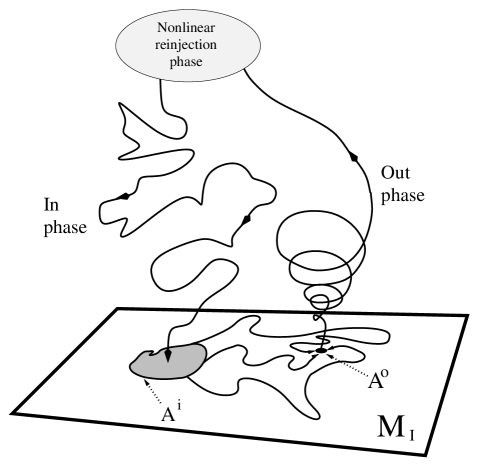
Figure 1: Schematic diagram showing a typical trajectory that is in–out intermittent to an invariant submanifold $M_{I}$, showing the ‘in’ and “out” phases. The invariant submanifold $M_{I}$ contains an invariant set that decomposes into a transversely attracting chaotic saddle $A^{i}$ and a transversely unstable periodic orbit $A^{o}$ that is an attractor within $M_{I}$. The ‘out’ phase is defined by the trajectory being within the isolating neighbourhood $U^{o}$ of $A^{o}$. In this case, the ‘in’ phase is modelled by a random walk in the logarithmic distance from $M_{I}$ whereas the “out” phase shows uniform exponential growth away from $M_{I}$, shadowing the unstable manifold of $A^{o}$.

There is now a good understanding of the statistical properties of on–off intermittency heagyetal1994 ; lai1996 ; venkataramanietal1996a ; cenysetal1997b and some properties of in–out ashwinetal1999 intermittency where they differ. Numerical support has also been obtained for both on–off ottetal1994 ; hataetal1997 ; dingetal1997 (for experimental evidence see hammeretal1994 ; yuetal1995 ) and in–out cat ; ctatb .

Both of these types of intermittency rely on the presence of invariant subspaces. In real systems, however, invariant subspaces are only expected to occur approximately; either as a result of the lack of precise symmetry or due to the presence of noise. This has motivated a number of studies of the effects of noise on the statistics of on–off intermittency plattetal1994 ; cenysetal1996 ; ashwinetal1997 ; lai1997 ; cenysetal1997a ; cenysetal1999 . Our aim here is to make an analogous study of the effects of noise in the case of in–out intermittency, by making a continuum version of the Markov model considered in ashwinetal1999 in order to highlight the similarities and differences. We do this by considering an analogue of the drift-diffusion model employed by ashwinetal1997 ; cenysetal1996 ; heagyetal1994 ; venkataramanietal1996a for on–off intermittency.

The structure of the paper is as follows. In Section II we derive and analyze a model of in–out intermittency that consists of a drift-diffusion equation with delay integral boundary conditions, based on extracting the important information from a dynamical model. We also discuss how to estimate parameters in the drift-diffusion model. Section III adapts these to include additive noise in the transverse variable as well as in the tangential variable. We predict new transitions in the dynamics on adding noise to the tangential variables. Section IV discusses the estimation of the parameters in the model and obtains scalings and transitions on changing the noise amplitude. These predictions are tested on a planar mapping given in ashwinetal1999 . Finally Section V gives a discussion and interpretation of the results.

II Modelling in–out intermittency

II.1 The dynamical model of in–out intermittency

Suppose that we have a dynamical system that evolves on ${\mathbf{R}}^{n}$, such that some subspace $M_{I}$ ($\dim(M_{I})<n$) of ${\mathbf{R}}^{n}$ is dynamically invariant. For definiteness we consider a dynamical system generated by iterating some smooth map $f:{\mathbf{R}}^{n}\rightarrow{\mathbf{R}}^{n}$, in which case $f(M_{I})\subseteq M_{I}$. If there is a minimal Milnor attractor $A$ for this system such that $A\cap M_{I}=A_{0}$ is not a minimal Milnor attractor for the system restricted to $M_{I}$, then we say the attractor is in–out intermittent ashwinetal1999 . (Recall that $A$ is a Milnor attractor if it has a basin with positive Lebesgue measure, such that any smaller invariant set has a basin with smaller measure. An attractor is minimal if it contains no proper subsets that are attractors).

Suppose now that $\gamma(t)$ is a typical trajectory in the basin of $A$, such that the $\omega$-limit set of $\gamma(t)$ is the attractor $A$. We assume that $A^{o}\subsetneq A_{0}$ is a Milnor attractor contained within $A_{0}$ for $f|_{M_{I}}$. We assume also that the only transversely stable set in $A_{0}$ is some $A^{i}\subsetneq A_{0}$ which is a repeller for $f|_{M_{I}}$. Each of the invariant sets $A^{i,o}$ is assumed to support invariant measures $\mu^{i}$ and $\mu^{o}$ that govern the behaviour of typical trajectories in $A$ on the approach to $A^{i,o}$.

We assume that $A^{i}$ is transversely attracting on average (i.e. its largest transverse Lyapunov exponent (L.E.) with respect to $\mu^{i}$ is $\lambda_{T}^{i}<0$) and $A^{o}$ is repelling on average (i.e. its largest transverse L.E. with respect to $\mu^{o}$ is positive). We refer to $A^{i}$ as the ‘in’ dynamics and $A^{o}$ as the ‘out’ dynamics for obvious reasons; see Figure 1 for a schematic representation.

II.1.1 Identifying the ‘in’ and ‘out’ phases

Suppose now that we have a projection $\Pi:{\mathbf{R}}^{n}\rightarrow M_{I}$ and a neighbourhood $U^{o}\subset M_{I}$ containing $A^{o}$, such that $f(U^{o})\supset U^{o}$ (i.e. it is absorbing for $f|_{M_{I}}$) minimalcomment . We identify a point $x$ in the phase space as being on ‘out’ phase if $\Pi(x)\in U^{o}$ and as being on the ‘in’ phase otherwise. Note that there is an arbitrary choice of neighbourhood $U^{o}$ and projection $\Pi$; however we will be interested in statistical properties of the ‘out’ phases that are independent of these.

For concreteness (and to correspond with examples studied later) we assume that the dynamics on $A^{o}$ is periodic and the dynamics on $A^{i}$ is chaotic (with many ergodic measures supported on $A^{i}$). However, in principle the same type of model applies as long as at least one of $A^{i}$ or $A^{o}$ is chaotic. We are interested in modelling the asymptotic fluctuation of the distance of some typical trajectory $\gamma(t)$ from $M_{I}$. Suppose we have a function

$$y(t)=\pi\gamma(t)$$ (1)

where $\pi:{\mathbf{R}}^{n}\rightarrow{\mathbf{R}}$ is a smooth function such that $\pi^{-1}(0)=M_{I}$. Then we say $\pi$ projects the phase space onto the transverse variable $y$. Clearly we have $\liminf_{t\rightarrow\infty}|y(t)|=0$ but $\limsup_{t}|y(t)|>0$. Moreover, such a transverse variable will, because of invariance of $M_{I}$, spend arbitrarily long times near $y=0$; the so-called laminar phases. The object of this paper is to give a statistical description of the behaviour of a generic $y(t)$ measuring the distance from $M_{I}$ for in–out intermittent dynamics.

II.2 A Fokker-Planck model for in–out intermittency

II.2.1 In terms of a logarithmic transverse variable, $z$.

We start with a transverse variable $y=\pi(\gamma)$ and set $z=-\ln|y|$; we model the behaviour of $z$ as follows. During the ‘in’ phase, we model the behaviour as though it is a linear skew product forced by the chaotic ‘in’ dynamics and we assume, by an appropriate scaling, that $|y|<1$ for all time. We model the behaviour as a drift-diffusion process in $z\geq 0$ with drift $-\lambda_{T}^{i}>0$ per unit time and diffusion $\beta^{2}$ per unit time subject to reflection boundary conditions at $z=0$. We assume that the trajectory leaks onto the ‘out’ phase at a rate $\epsilon>0$ per unit time (this is given by the most positive tangential L.E. of $\mu_{i}$).

On the ‘out’ phases we assume that there is a fixed linear expansion forced by the periodic ‘out’ dynamics. This translates to a deterministic growth in the $z$ variable at a rate $-\lambda_{T}^{o}<0$. Once $z$ reaches $0$ we assume that the trajectory is forced to re-inject to the ‘in’ dynamics. For convenience, from here on we define

$$c = \lambda_{T}^{o},$$

$$\lambda = \lambda_{T}^{i}$$

and note that $c>0$, whereas $\lambda$ can be positive or negative in what follows.

Let the probability density at time $t$ of the distribution of $z$ values in $(z,z+dz)$ on the ‘in’ phase be given by $P(z,t)dz$ and those on the ‘out’ phase be given by $R(z,t)dz$. Our model translates to a forward Kolmogorov equation for $P$ of the form

$${\frac{\partial{P}}{\partial{t}}}={\frac{\partial{\Gamma}}{\partial{z}}}-\epsilon P$$ (2)

where the second term on the right hand side represents the leakage into the ‘out’ phase and

$$\Gamma(z,t)=\beta^{2}/2{\frac{\partial{P}}{\partial{z}}}+\lambda P$$ (3)

represents the flux of trajectories at $(z,t)$. The dynamics for $R$ on the ‘out’ phases is simply given by the hyperbolic equation

$$\left({\frac{\partial{}}{\partial{t}}}-c{\frac{\partial{}}{\partial{z}}}\right)R=\epsilon P.$$ (4)

This equation can be solved exactly to give

$$R(z,t)=\frac{\epsilon}{c}\int_{z}^{\infty}P\left(x,t-\frac{x-z}{c}\right)\,dx,$$ (5)

which is unique up to the addition of an arbitrary function $\xi(x+ct)$. The total probability of being in the ‘in’ or ‘out’ chain is then given by

$$\Phi^{i}(t)=\int_{0}^{\infty}P(z,t)\,dz,~{}~{}~{}\Phi^{o}(t)=\int_{0}^{\infty}R(z,t)\,dz$$ (6)

respectively. We assume also that

$$\Gamma(0,t)+cR(0,t)=0$$ (7)

at $z=0$, which corresponds to reinjecting trajectories reaching $z=0$ of the ‘out’ chain back into the ‘in’ chain. If we define the total overall probability of being in the ‘in’ and ‘out’ chains by

$$\Phi(t)=\Phi^{i}(t)+\Phi^{o}(t)$$ (8)

then we have

$${\frac{\partial{\Phi}}{\partial{t}}} = \int_{0}^{\infty}\left({\frac{\partial{P}}{\partial{t}}}+{\frac{\partial{R}}{\partial{t}}}\right)\,dz$$

$$= \int_{0}^{\infty}\left({\frac{\partial{\Gamma}}{\partial{z}}}-\epsilon P+c{\frac{\partial{R}}{\partial{z}}}+\epsilon P\right)\,dz$$

$$= \Gamma(0,t)+cR(0,t)$$

$$= 0,$$

implying that $\Phi(t)$ is a constant. We therefore stipulate that by normalization

$$\Phi(t)=1$$ (10)

for all $t$. Thus the Fokker-Planck model of in–out intermittency (in the absence of noise) is the closed system consisting of the linear equation (2) for $P(z,t)$ on $z\in[0,\infty)$ subject to the delay integral boundary condition (7) and normalization condition (10).

II.2.2 In terms of the transverse variable, $y$.

The drift-diffusion model in the variable $z$ can be translated into one for the original transverse variable $y=e^{-z}$ as follows: Let the probability density at time $t$ of the distribution of $y$ values in $(y,y+dy)$ on the ‘in’ phase be given by $Q(y,t)dy$ and those on the ‘out’ phase be given by $S(y,t)dy$. Note that (assuming $y>0$)

$$P=\left|\frac{dy}{dz}\right|Q=yQ,~{}~{}~{}R=\left|\frac{dy}{dz}\right|S=yS$$ (11)

and so the system governing $Q(y,t)$ and $S(y,t)$ is given by

$${\frac{\partial{Q}}{\partial{t}}} = \frac{\beta^{2}}{2}{\frac{\partial{}}{\partial{y}}}\left(y{\frac{\partial{}}{\partial{y}}}(yQ)\right)-\lambda{\frac{\partial{}}{\partial{y}}}(yQ)-\epsilon Q$$ (12)

$$S = \frac{\epsilon}{cy}\int\limits_{0}^{y}Q\left(w,t+\frac{\ln y-\ln w}{c}\right)\,dw,$$ (13)

with the boundary conditions given by

$$1 = \int_{0}^{1}\left[Q(y,t)+S(y,t)\right]\,dy$$ (14)

$$0 = \frac{\beta^{2}}{2}(y{\frac{\partial{}}{\partial{y}}}(yQ))-\lambda yQ+S~{}~{}\mbox{ at }y=0$$ (15)

Observe that in terms of these variables we have

$$\Phi^{i}=\int_{0}^{1}Q(y,t)\,dy,~{}~{}~{}~{}\Phi^{o}=\int_{0}^{1}S(y,t)\,dy.$$ (16)

Moreover we find

$${\frac{\partial{\Phi^{i}}}{\partial{t}}}=\Gamma(0,t)-\epsilon\Phi^{i}.$$ (17)

II.3 Stationary distributions; noise free

Steady solutions $P(z,t)=p(z)$ of (2) will satisfy

$$\frac{\beta^{2}}{2}p_{zz}+\lambda p_{z}-\epsilon p=0$$ (18)

with boundary conditions given by (7) and (10). This can easily be solved to give a solution

$$p(z)=Ae^{\mu_{-}z}+A_{+}e^{\mu_{+}z}$$ (19)

where

$$\mu_{\pm}=\frac{-\lambda\pm\sqrt{\lambda^{2}+2\epsilon\beta^{2}}}{\beta^{2}}.$$ (20)

Note that if $\epsilon>0$, then $\sqrt{\lambda^{2}+2\epsilon\beta^{2}}>|\lambda|$ and so $\mu_{-}<0$ and $\mu_{+}>0$ always, as long as $\epsilon>0$. A similar result was found for the Markov model of in–out intermittency discussed in ashwinetal1999 . We therefore write

$$\mu=\mu_{-},~{}~{}~{}A=A_{-}$$ (21)

and note that the only solutions of (18) with finite mass are such that $A_{+}=0$. Calculating the stationary mass in the ‘out’ chain we have

$$r(z)=Be^{\mu z}$$ (22)

where $-c\mu B=\epsilon A$ and so $B=-\frac{\epsilon}{c\mu}A$. This means that

$$\Phi^{i}=\frac{A}{\mu},~{}~{}~{}\Phi^{o}=\frac{B}{\mu}.$$ (23)

Normalizing so that the total mass is unity we have

$$1=\frac{A}{\mu}+\frac{B}{\mu}$$ (24)

which gives

$$A=\frac{c\mu^{2}}{c\mu-\epsilon}\qquad B=\frac{\epsilon\mu}{\epsilon-c\mu},$$ (25)

thus ensuring that the boundary condition is also satisfied

$$\begin{array}[]{l}\Gamma(0,t)+cR(0,t)=\\ \left(\frac{\beta^{2}\mu^{2}}{2}+\lambda\mu-\epsilon\right)Ae^{\mu t}=0.\end{array}$$ (26)

These steady exponential distributions correspond to algebraic distributions for the $Q(y)$ and $S(y)$. In Section IV.1 we discuss how the free parameters in this model can be estimated from the dynamical data.

II.4 Contrasts with on–off intermittency

Note that one could take a simpler dynamical model in the form of a drift-diffusion equation but with no differentiation into ‘in’ and ‘out’ phases. This is equivalent to assuming that $\epsilon=0$ in the model (i.e. reducing it to an on–off process) and leads to an exponential probability distribution of the form

$$p(z)=Ae^{-\frac{\lambda}{2\beta^{2}}z}$$ (27)

However, estimation of the constants $\lambda$, $\beta$ presents a problem as we will discuss in Section IV.2.

For in–out intermittency, the ‘out’ phase is distinct from other invariant sets that we may choose within the invariant subspace in the following sense. There are constants $E,F>0$ such that if any trajectory enters the ‘out’ phase at a distance $d$ from the invariant subspace then there is a minimum residence time in the ‘out’ phase given by

$$E-F\ln d.$$ (28)

In particular the minimum ‘out’ phase residence time goes to infinity as $d\rightarrow 0$.

III A model for in–out intermittency with additive noise

The model of Section II can now be easily generalized to model in–out intermittency in the presence of unbiased additive noise. At first we will investigate the case where the noise is added only to the transverse variables and later examine the case of noise added to tangential variables. It appears that noise in the transverse variables affects scalings in a regular manner; whereas noise in the tangential variables can lead to transitions as ‘in’ and ‘out’ phases merge.

III.1 Additive noise in the transverse variables

In presence of additive noise in the transverse variables, we use a similar approach to that of Ashwin & Stone ashwinetal1997 and Venkataramani et al. venkataramanietal1996a to obtain a Fokker-Planck model of the form

$${\frac{\partial{Q}}{\partial{t}}} = -\lambda{\frac{\partial{(Qy)}}{\partial{y}}}+\frac{\beta^{2}}{2}{\frac{\partial{}}{\partial{y}}}\left(y{\frac{\partial{(Qy)}}{\partial{y}}}\right)+$$

$$\frac{\sigma^{2}}{2}{\frac{\partial{{}^{2}Q}}{\partial{y^{2}}}}-\epsilon Q,$$

which is similar to (12) apart from the diffusion term at a rate $\sigma^{2}/2$ corresponding to the additive noise.

III.1.1 Steady state with additive noise

We obtain a steady state probability density distribution in the in–out case, by calculating the contributions from both ‘in’ and ‘out’ chains separately.

For the contribution from the ‘in’ chain we proceed by looking at the steady state counterpart of the equation (III.1) obtained by demanding $Q(y,t)=q(y)$,

$$-\lambda\frac{d(yq)}{dy}+\frac{\beta^{2}}{2}\frac{d}{dy}\left(y\frac{d(yq)}{dy}\right)+$$ (30)

$$\frac{\sigma^{2}}{2}\frac{d^{2}q}{dy^{2}}-\epsilon q=0$$

which can be written in the form

$$\frac{1}{2}\left(\beta^{2}y^{2}+\sigma^{2}\right){\frac{d{{}^{2}q}}{d{y^{2}}}}+\left(\frac{3}{2}\beta^{2}-\lambda\right)y{\frac{d{q}}{d{y}}}$$ (31)

$$+\left(\frac{\beta^{2}}{2}-\lambda-\epsilon\right)q=0.$$

To solve this equation we recall that the case with $\epsilon=0$, corresponding to on–off intermittency, is solvable explicitly (see venkataramanietal1996a ) with the solution

$$q(y)=A(\beta^{2}y^{2}+\sigma^{2})^{\frac{\xi-1}{2}}$$ (32)

where $\xi=\frac{2\lambda}{\beta^{2}}$. In the case of in–out intermittency with $\epsilon\neq 0$, we proceed by employing the (singular at $\sigma=0$) change of variable

$$x=-\frac{\beta^{2}}{\sigma^{2}}y^{2},$$ (33)

to rewrite the equation (31) in the form

$$x(1-x)\frac{d^{2}q}{dx^{2}}+\left(\frac{1}{2}-x\left(1+\frac{\beta^{2}-\lambda}{\beta^{2}}\right)\right)\frac{dq}{dx}$$ (34)

$$-\frac{\beta^{2}-2\lambda-2\epsilon}{4\beta^{2}}q=0.$$

This equation can be solved in terms of hypergeometric functions

$$q=A(\beta,\sigma,\lambda,\epsilon)F_{(\alpha_{+},\alpha_{-},1/2,x)}$$ (35)

where

$$\alpha_{\pm}=\frac{\beta^{2}-\lambda\pm\sqrt{\lambda^{2}+2\beta^{2}\epsilon}}{2\beta^{2}}=\frac{1+\mu_{\pm}}{2},$$ (36)

with $\mu_{\pm}$ as before, and

$$F_{(a,b,c,z)}=\frac{\Gamma(c)}{\Gamma(b)\Gamma(c-b)}\int\limits_{0}^{1}\frac{t^{b-1}(1-t)^{c-b-1}}{(1-tz)^{a}}dt.$$ (37)

If $|x|\gg 1$, $x<0$ and $Real(a-b)=2\sqrt{\lambda^{2}+2\beta^{2}\epsilon}>0$, this solution can be approximated by using

$$\begin{array}[]{l}F_{(\alpha_{+},\alpha_{-},1/2,x)}\\ \approx(1-x)^{-\alpha_{-}}\times\frac{\Gamma(1/2)\Gamma(\sqrt{\lambda^{2}+2\beta^{2}\epsilon)}/(2\beta^{2}))}{\Gamma(\alpha_{+})\Gamma(1/2-\alpha_{-})}\\ =K(1-x)^{-\alpha_{-}},\end{array}$$ (38)

for some constant $K$. This then gives

$$q(y)\approx A\left(\sigma^{2}+\beta^{2}y^{2}\right)^{-\frac{1}{2}-\frac{\mu}{2}},$$ (39)

where $A=A(\beta,\sigma,\lambda,\epsilon)$ is the normalisation constant, and $\mu=\mu_{-}$ as before, is valid for small $|y|$.

For the ‘out’ chain, the steady state probability density distribution can be obtained from (13) by employing the steady state form of $Q$ in the integral in this expression to compute $s(y)$

$$s(y)=\frac{\epsilon}{cy}\int_{0}^{y}q(w)\,dw.$$ (40)

The overall steady state probability density distribution is then given by the sum of these two contributions $q(y)+s(y)$.

III.1.2 Scaling of the mean first crossing time

To begin with, we recall that for unbiased noise on the variable $y$, the mean is clearly

$$E(y)=0.$$ (41)

To determine the mean crossing time through $y=0$, we require $A$ which can be computed assuming there are no-flux boundary conditions at $y=\pm 1$ (with linear behaviour up to this point), to give

$$\int_{|y|<1}P(y)\,dy=1.$$ (42)

Away from a blowout bifurcation point, it is not so easy to obtain an explicit expression for $A$ and thus for the variance $var(y)$. However, in the low noise limit, $\sigma\ll\beta$, we can approximate the stationary density (39) by the continuous function

$$q(y)\approx\left\{\begin{array}[]{ll}A\sigma^{-1-\mu}{}{}&\mbox{ for }~{}|y|<\sigma/\beta,\\ A\left(\beta y\right)^{-1-\mu}{}{}&\mbox{ for }~{}\sigma/\beta<|y|<1,\end{array}\right.$$ (43)

and $s(y)$ is calculated from (40) as

$$\begin{array}[]{l}s(y)\approx\frac{\epsilon A}{c}\times\\ \left\{\begin{array}[]{ll}\sigma^{-1-\mu}{}{}&\mbox{ for }~{}|y|<\sigma/\beta,\\ \frac{1}{-\mu}\left[(\beta y)^{-1-\mu}-\frac{\sigma^{-\mu}(1+\mu)}{\beta y}\right]{}{}&\mbox{ for }~{}|y|>\sigma/\beta.\end{array}\right.\end{array}$$ (44)

In order to compare these results with those in the case of on–off, we proceed by computing the value of the normalisation constant $A$. This is given by computing (42) with $P(y)=q(y)+s(y)$ and gives, for this approximation,

$$\begin{array}[]{l}A=c\mu^{2}\beta\left[(\epsilon-c\mu)(\beta^{-\mu}-\sigma^{-\mu})\right.\\ ~{}~{}~{}\left.-\sigma^{-\mu}\mu(\epsilon\ln\frac{\sigma}{\beta}(1+\mu)+(c+\epsilon)\mu))\right]^{-1}.\end{array}$$ (45)

In the limit $\epsilon\rightarrow 0$ this expression reduces to the on-off case

$$A=\frac{\mu\beta}{\sigma^{-\mu}(1+\mu)-\beta^{-\mu}}$$ (46)

equivalent to that found in ashwinetal1997 . Using the approximation that the stationary distributions $q(y)$ and $s(y)$ are approximately constant for $|y|<\sigma$, the instantaneous flux from $y>0$ to $y<0$ can then be estimated as

$${\cal F}=\frac{1}{2}\sigma(q(0)+s(0))$$ (47)

where, as in ashwinetal1997 , we have assumed that with unbiased additive noise approximately half of all initial points in $[0,\sigma]$ will cross over within the next time unit. We can compute ${\cal F}$, by using the above solutions (43) and (44) together with (45), to obtain

$$\begin{array}[]{l}{\cal F}=\sigma^{-\mu}\mu^{2}\beta(c+\epsilon)\left[2((\epsilon-c\mu)(\beta^{-\mu}-\sigma^{-\mu})\right.\\ ~{}~{}\left.-\sigma^{-\mu}\mu(\epsilon\ln\frac{\sigma}{\beta}(1+\mu)+(c+\epsilon)\mu))\right],\end{array}$$ (48)

which in the limit $\epsilon\rightarrow 0$ reduces to the on–off formula

$${\cal F}=\frac{1}{2}\frac{\sigma^{-\mu}\beta\mu}{\sigma^{-\mu}(1-\mu)+\beta^{-\mu}}.$$ (49)

This allows the calculation, in the in–out case, of the mean first crossing time given by $M=1/{\cal F}$ analogous to ashwinetal1997 , i.e.

$$\begin{array}[]{l}M=\frac{2}{\mu^{2}\beta(\epsilon+c)}\left((\epsilon-c\mu)((\frac{\beta}{\sigma})^{-\mu}-1)\right.\\ \left.-\epsilon\mu\ln\frac{\sigma}{\beta}(1+\mu)+(c+\epsilon)\mu^{2})\right).\end{array}$$ (50)

Considering the case where $\epsilon$ is asymptotically small (i.e. small leakage of the ‘in’ dynamics) we have

$$M=\frac{2}{\beta}\left[1+\frac{1}{\mu}\left(\left(\frac{\beta}{\sigma}\right)^{-\mu}-1\right)+O(\epsilon,\mu)\right].$$ (51)

Furthermore, if we are close to marginal stability on the ‘in’ chain, $\lambda=0$, we have $\mu=-\frac{\sqrt{2\epsilon}}{\beta}$ and so in the limit $\epsilon\rightarrow 0$ we recover the expression in ashwinetal1997 , namely

$$M\approx\frac{2}{\beta}+\frac{2}{\beta\mu}\left(\left(\frac{\beta}{\sigma}\right)^{-\mu}-1\right)+O(\sqrt{\epsilon}),$$ (52)

with an order $\sqrt{\epsilon}$ correction. Similarly, expressions can be obtained for other limiting cases; we give one such scaling with the numerical results in a later section.

We have attempted to find the scaling of the mean laminar length with noise intensity, analogous to cenysetal1996 for on–off intermittency. However, the need to distinguish between the dynamics of the ‘in’ and and ‘out’ phases means that we cannot easily reduce the problem to a single ordinary differential equation with the consequence that we have so far not been able to obtain an expression as compact as that for on–off. However, in principle the Fokker-Planck model (III.1) contains all the necessary information to compute this.

III.2 Added noise in tangential variables

It has been noted plattetal1994 that the addition of noise to tangential variables in the case of on–off intermittency has only a minor effect on the dynamics. This can be understood if the attractor within $M_{I}$ is stochastically stable, i.e. if the probability density with noise limits to the probability density of the natural measure in the case of no noise. In the case of in–out intermittency, on the other hand, there will be a threshold of noise amplitude beyond which the fine structure in the invariant subspace is destroyed.

To be more precise, suppose we have a dynamical scenario as described in Section II.1 and the ‘out’ dynamics $A^{o}$ has a basin such that the largest neighbourhood of $A^{o}$ contained in the basin has radius $\rho>0$, and the dynamics is uniformly contracting onto $A^{o}$ in the tangential direction at a rate $\eta<0$. We can model the approach to $A^{o}$ along its weak stable manifold by a map $x_{n+1}=e^{\eta}x_{n}$ where $x$ corresponds to the distance from $A^{o}$. Perturbing this map by i.i.d. noise $\xi_{n}$ that is uniformly distributed in $[-\sigma\sqrt{3},\sigma\sqrt{3}]$ (such that the variance is $\sigma$) we obtain an iterated function system of the form $x_{n+1}=e^{\eta}x_{n}+\xi_{n}$. We can see that fluctuations will drive $x_{n}$ to exceed $\rho>0$ if

$$\sigma>\rho(1-e^{\eta})/\sqrt{3}.$$ (53)

Consequently we expect that the ‘out’ phase and ‘in’ phase can no longer be distinguished once the noise has reached the order of this threshold.

IV Numerical results and scalings

In order to test our model of in–out intermittency (with and without noise) we consider a simple model mapping of the plane introduced in ashwinetal1999

$$f(x,y)=(rx(1-x)+sxy^{2},1.82e^{-x}y-y^{3}),$$ (54)

which has two parameters $r\in[0,4]$ and $s\in{\mathbf{R}}$. We can view this as a map of ${\mathbf{R}}^{2}$ to itself that leaves $M_{I}={\mathbf{R}}\times\{0\}$ invariant. If $s=0$, the map has the form of a skew product over the dynamics in $x$, i.e. it can be written as

$$f(x,y)=(h(x),g(x,y))$$ (55)

with

$$h(x)=rx(1-x)\ \mbox{and}\ g(x,y)=1.82e^{-x}y-y^{3},$$ (56)

where $x\in M_{I}$. If we fix $r$ and vary $s$ we see that the latter two parameters do not affect the map restricted to $M_{I}$ and so are normal parameters for the system restricted to $M_{I}$.

An example of the behaviour of the transverse and tangential L.E.s around a window of periodicity for which the map (54) shows in–out intermittency is depicted in Figure 2.

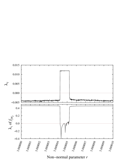
Figure 2: L.E. $\lambda_{1}$ in the tangential direction and $\lambda_{T}$ in the transverse direction for the map (54) with $s=-0.3$ and varying $r$. Initial conditions chosen to evolve to the attractor in $M_{I}$, i.e. with $y=0$. Observe the ‘periodic window’ coincides with transverse instability of the attractor in $M_{I}$. In this region one can find in–out intermittent attractors for the full map that are not contained in $M_{I}$. Note that the attractor with transverse L.E. approximately $-0.005$ remains as a chaotic saddle during the periodic window; this saddle controls the in-phase.

We have also shown in Figure 3 a typical time series corresponding to the in–out intermittent behaviour produced by this map. The top panel clearly demonstrates windows of periodic locking (corresponding to the ‘out’ phases), interspersed by chaotic windows (corresponding to the ‘in’ and ‘reinjection’ phases). One can also clearly see from the bottom panel the exponential growth in the amplitude of the transverse variable $y$ during the ‘out’ phases.

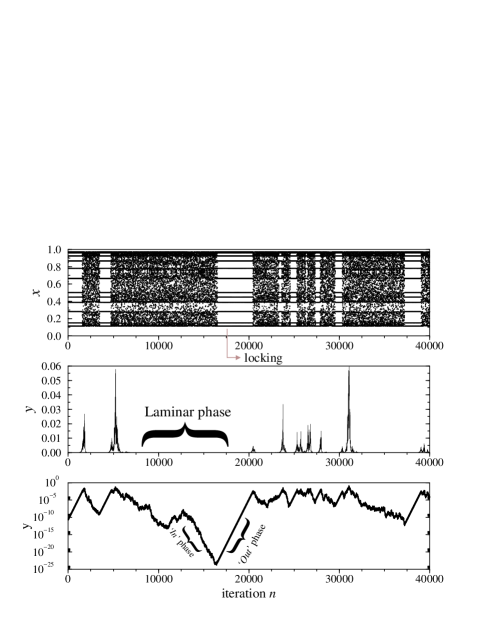
Figure 3: Example of time series generated by iterating (54) from a randomly chosen initial condition, after transient effects have died out. The bottom plot shows $y$ in a logarithmic scale, and the top second and the middle plots show $x$ and $y$ on linear scales. Parameter values are fixed at $(r,s)=(3.88615,-0.3)$.

To study the effects of noise on in–out intermittency, it is informative to compare it with the analogous studies of on–off. To do this we chose two sets of values for the control parameters $r$ and $s$ (namely $r=3.8800045$, $s=-0.3$ and $r=3.82786$, $s=0$) in the map (54), corresponding to in–out and on–off intermittencies respectively. We perturbed the map with uniform noise on $[0,\zeta]$ for the $x$ dynamics and $[-\zeta,\zeta]$ for the $y$ dynamics. We have considered the two cases above where the noise is imposed (I) on the tangential variable $x$ and (II) on the transverse variable $y$.

IV.1 Estimating the parameters for the noise-free model

Observe that the noise-free model for in–out intermittency, after a suitable non-dimensionalisation of the transverse variable has four parameters; $\lambda$, $\beta$, $\epsilon$, $c$ with an arbitrary choice for application of the boundary condition at $y=1$ after a suitable rescaling of $y$. We estimate these parameters as follows. We take a trajectory such that the transient has decayed and we can identify parts of the trajectory as ‘in’ or ‘out’ phase by choice of a suitable $U^{0}$. For the map (54) with $r=3.8800045$ and $s=-0.3$, we can define the trajectory $(x_{n},y_{n})$ as being in the ‘out’ phase if

$$\min\{|x_{n}-p_{i}|~{}:i=1\ldots 12\}<10^{-4}$$

i.e. if it approaches the period 12 attractor $\{p_{i}~{}:i=1\ldots 12\}$ for $y=0$ to within $10^{-4}$. Using this criterion, we have depicted in Figure 4 the values of the transverse variable $y$ at the entrance and exit of the ‘out’ phases identified by this procedure. Note that the exit point is more or less constant while the entrance point is distributed in a manner consistent with exponential distribution in $z=-\ln|y|$ (see Figure 5).

Figure 4: A plot of $\ln(y)$ at the entrance at the $n$th period, showing the value at the start of the ‘out’ phase (lower point) and that at the exit from the ‘out’ phase (upper point) for in–out intermittency, plotted against event number. Observe that exit never occurs closer than a certain distance from the invariant manifold at $\ln|y|=-\infty$. The events appear to be independent and uniformly distributed in time.

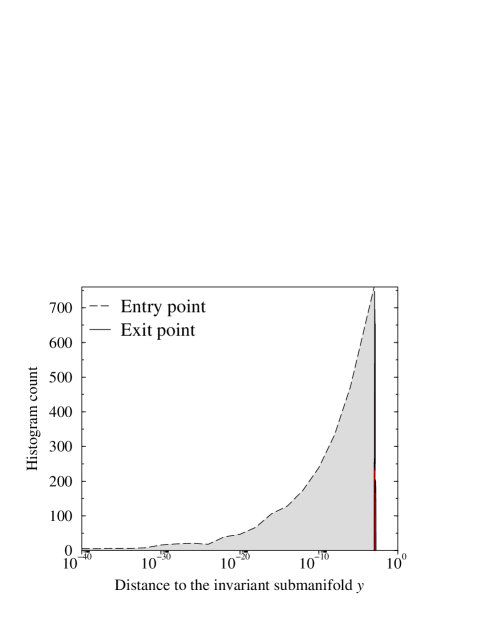
Figure 5: A histogram of the entrance to the ‘out’ phases and the exit from the ‘out’ phases for in–out intermittency for the trajectory considered in Figure 4.

IV.1.1 Estimating $\epsilon$.

Since our model implies that probability $\Phi^{i}$ decays from the ‘in’ phase at a rate $\epsilon$ per unit time, this corresponds to an exponential distribution of lengths of the ‘in’ phases with average length of ‘in’ phase being $1/\epsilon$. Hence

$$\epsilon=\frac{1}{L_{i}},$$ (57)

where one can easily approximate the quantity

$$L_{i}=\{\mbox{Average length of `in' phase}\}.$$ (58)

For the map (54) with $r=3.8800045$ and $s=-0.3$, we estimate $L_{i}\sim 5600\pm 200$ and so $\epsilon\sim 0.00018\pm 5\times 10^{-6}$; see Figure 6.

Figure 6: The histogram of the lengths of the ‘in’ phases for the trajectory considered in Figure 4. This was used to calculate $\epsilon$ from the inverse of the average length of the ‘in’ phases $\tau$.

IV.1.2 Estimating $c$.

This is simply the largest transverse L.E. for $A^{o}$, and can in some cases be obtained analytically. It can also be estimated numerically as the average growth rate of $|y|$ during the ‘out’ phases. For the example of in–out intermittency discussed above we can compute $c$ to be

$$c\sim\frac{0.1434}{12}=0.01195\pm 10^{-5}$$ (59)

which is the transverse L.E. of the attracting period 12 orbit in $M_{I}$.

IV.1.3 Estimating $\lambda$ and $\beta$.

These parameters can be obtained by examining the average rate of growth during ‘in’ phases. More precisely, we pick a threshold $z_{th}=-\ln(y_{th})$ which is large and time $T>0$, and then examine all instances where the trajectory starts in the ‘in’ phase at $z(t_{0})=z_{th}$ and remains in the ‘in’ phase for at least a time $T$.

Note that $T$ needs to be chosen so that $z(t)$ does not get too small (i.e. $y(t)$ does not get too large) for $t_{0}<t<t_{0}+T$ and one needs to be careful to avoid limiting the trajectory in such a way that may condition the mean or variance we are trying to measure, for example by choosing the threshold in $y$ to be too large, or by choosing $T$ to be so long that one will enter the nonlinear range.

Subject to this, we can approximate $\lambda$ as the average value of

$$(\ln(y(t_{0}+T))-\ln(y(t_{0})))/T$$ (60)

over this ensemble of ‘in’ phases. Similarly $\beta$ can be found as the standard deviation of this quantity from its mean value, per unit time. For the example of in–out intermittency in map (54) discussed above, we used up to 20,000,000 points of the trajectory, with $T=100$ and an ensemble of in-phase segments of the same trajectory with $z_{th}\sim 30$ to find that

$$\lambda\sim-0.0042,~{}~{}~{}\beta\sim 0.0135.$$ (61)

where there is an expected maximum error of approximately $5\%$ (see Figure 7).

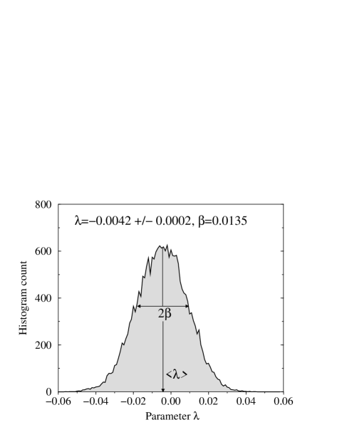
Figure 7: Histogram of the distribution of calculated values of $\lambda$ and estimation of $\lambda$ and $\beta$ from the in phases for the trajectory considered in Figure 4. (see text for details).

IV.1.4 Check: an independent estimate of $\mu$.

Recall that the ratio of the times spent in the ‘in’ to the ‘out’ phases can be obtained from the stationary distributions in the form

$$R_{io}=\frac{\Phi^{i}}{\Phi^{o}}=\frac{A}{B}=-\frac{c\mu}{\epsilon}.$$ (62)

Using our knowledge of $\epsilon$ and $c$ we can easily obtain $\mu$ and check this against the theoretical prediction (20), given approximations of the quantities $\Phi^{i}=$ { Asymptotic proportion of time spent on the ‘in’ phase } and $\Phi^{o}=$ {Asymptotic proportion of time spent on the ‘out’ phase} $=1-P^{i}$. For the case of in–out intermittency considered above, the above estimates of the parameters imply that

$$\mu\sim-0.0451,$$

which allow us to obtain a numerical estimate for $R_{io}\sim 3.02$ with an estimated maximum error of $15\%$.

Using instead the measured ratio of average length of ‘in’ to ‘out’ phases we obtain an estimate for $R_{io}=2.56$ with an estimated maximum error of approximately $10\%$. These two estimates of $R_{io}$ clearly agree to within estimated maximum error.

Note that the neighbourhood $U^{0}$ of the ‘out’ dynamics $A^{0}$ must be chosen such that the $U^{0}\cap M_{I}$ is forward invariant. It can be chosen as small as desired, though if it is very small then we will not recognize ‘out’ phases unless they come very close to $M_{I}$.

IV.2 Lack of fit to a Fokker-Planck model of on–off intermittency

It is interesting to note that it is not possible to fit in–out intermittent dynamical data by an on–off model. This is because the on–off model requires only two parameters, the transverse L.E. $\lambda\geq 0$ and its variance per unit time $\beta^{2}$. If we examine the attractor in $M_{I}$, we can compute a positive L.E. ($c$ above), but the variance would be zero. Alternatively we can compute the ‘in’ phases as discussed above and obtain both a $\lambda$ and a $\beta^{2}>0$, but in that case $\lambda<0$. Thus either choice will be invalid.

Alternatively one could compute $\lambda/\beta^{2}$ from the scaling of the probability density near $y=0$, but then it is not clear how to make a sensible choice for $\lambda$ or $\beta$ and therefore we can determine only one of the parameters in the model.

IV.3 Probability distribution for the case with noise

Figure 8 shows the results of three distinct ways of calculating the asymptotic probability distribution function (pdf) of $q(y)$; resp. $s(y)$, for a fixed noise level (in this case $\zeta_{y}=10^{-8}$): from the direct integration of (31) using the estimate values of the parameters $\epsilon$, $c$, $\lambda$ and $\beta$; from the full analytical solution (31) and finally from the direct numerical measure of the pdf of $Q(y)$.

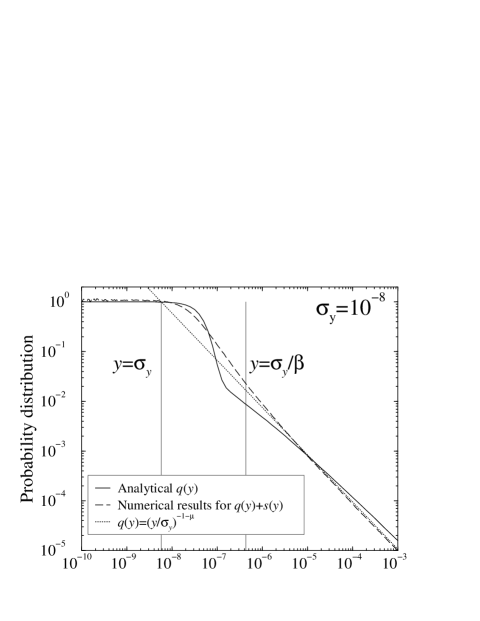
Figure 8: Histogram of the pdfs $q(y)$ on the in-phase and $s(y)$ on the out-phase as a function of the transverse variable $y$ for transverse added noise $\sigma_{y}=10^{-8}$ for the examples of in–out intermittency in (54) discussed in the text. Note that the analytical solution joins the two regions, $|y|<\sigma$ and $|y|>\sigma/\beta$ by means of an internal boundary layer. Note that any algebraic scaling of $q(y)\approx y^{\alpha}$ implies the same scaling for $s(y)$.

We have also plotted in Figure 9 the influence of different values of the noise level $\zeta$ on the transverse variable $y$ in the pdf of $Q(y)$, for both in–out and on–off cases, and discuss the behaviour in the figure caption.

Figure 9: Histogram of the pdf $Q(y)$ as a function of the transverse variable $y$ for transverse added noise for the examples of on–off and in–out intermittency in (54) discussed in the text. Observe that there is a power law scaling across a wide range of $y$ that changes to a constant smooth density (plateau) for very small $y$. The turning point corresponds, as expected, to the noise level imposed; the response of on–off and in–out intermittency to the addition of transverse noise can be seen to be similar.

IV.4 Length of the average laminar phase as a function of noise

IV.4.1 Noise on tangential variable

We calculated for the map (54) the scaling of the length of the average laminar phases, as a function of the noise level $\zeta$. Our results are depicted in Figure 10. As can be seen, in this case there is a significant difference between the on–off and in–out cases. While both show very similar behaviours for low noise levels, at higher noise levels, the behaviours show some distinct differences. In particular, average laminar sizes corresponding to the in–out case drop off rather suddenly, whereas for the on–off case there is an increase in the size of the average laminar phases before it too drops off suddenly. This corresponds well with the discussion in Section III.2, where we argued that in the case of in–out, a sudden change in dynamics would be expected at a certain noise level. For the map considered here, we observe that the local basin of the ‘out’ dynamics is of the order $10^{-6}$ which from (53) would suggest a noise threshold that is at most $10^{-6}$.

Figure 10: The difference between on–off and in–out intermittency shows itself qualitatively in the behaviour of the average laminar phase size as a function of the noise level $\zeta=\sqrt{3}\sigma$ for noise addition to the tangential variable $x$. This illustrates the case for tangential and transverse added noise to map (54). The noise on $x$ is uniformly distributed in the range $[0,\zeta_{x}]$, while that on $y$ is in the range $[-\zeta_{y},+\zeta_{y}]$. The parameter values are $r=3.8800045$, and $s=-0.3$. The decay for noise on $x$ in the in–out case corresponds to the $x$-perturbation getting large enough to destroy the basin of attraction of the ‘out’ dynamics; by contrast the addition of tangential noise to on–off intermittency only makes a difference at much larger levels.

Also shown on this Figure are the results for the case of on–off intermittency for the same map at a different parameter value (see caption). One would expect a decrease in the average length of laminar phases until $\sigma$ is of the same order of the threshold defining the laminar phases, which in this case is $\sim 10^{-3}$. This is to be contrasted with the in–out case, where the drop off is more sudden and occurs at much lower noise levels (i.e $\sim 10^{-6}$). This level of noise seems to be enough to disrupt the periodic attractor in the invariant submanifold and it is interesting to note that the noise level at which this occurs is of the same order of magnitude as the size of the parameter window of periodicity.

IV.4.2 Noise on transverse variable

For the noise on the transverse variable, on–off and in–out behave quite similarly in terms of the average laminar phases, showing a smoother decay than the case (I), with the dramatic drop occurring around $10^{-4}$, which is closer to the threshold level. As can be seen from Figure 11, the ‘out’ chains, initially dominant, decay rapidly, while the ‘in’ chains are on average of the same size for a wide band of noise levels $\sigma$, up to values of about $10^{-6}$. Note also that the actual percentage of time spent in the ‘in’ chains actually increases at high noise levels before decaying to zero, while the time spent in the ‘out’ chains decreases monotonically.

Figure 11: Comparison of the average length of laminar phase, ‘in’ phase and ‘out’ phase as a function of the noise level $\sigma$ for addition of transverse noise in the variable $y$; parameter values are $r=3.8800045$ and $s=-0.3$.

IV.4.3 Average mean crossing time through $y=0$

One can similarly analyze for the model the average mean crossing time $M$ through $y=0$ in presence of noise on $y$ (case (II)). For positive transverse L.E. ($\lambda_{T}>0$), that is for parameter values away from the blowout point, one expects for the case of on–off a typical growth given by ashwinetal1997

$$M\approx\frac{\beta^{1+\xi}}{\lambda}\sigma^{-\xi}+O(1).$$ (63)

For the on–off case, ashwinetal1997 predicts that at blowout point the scaling has the asymptotic form ($\lambda\rightarrow 0$)

$$M\approx-\frac{2\ln\sigma}{\beta}+O(1).$$ (64)

In the in–out case we find the scaling for small $|\sigma|$, can be approximated from the expansion of (50) in $\sigma$, considering $\lambda_{T}\mathrel{\mathchoice{\vbox{\offinterlineskip\halign{\hfil$\displaystyle#$\hfil\cr>\cr\sim\cr}}}{\vbox{\offinterlineskip\halign{\hfil$\textstyle#$\hfil\cr>\cr\sim\cr}}}{\vbox{\offinterlineskip\halign{\hfil$\scriptstyle#$\hfil\cr>\cr\sim\cr}}}{\vbox{\offinterlineskip\halign{\hfil$\scriptscriptstyle#$\hfil\cr>\cr\sim\cr}}}}0$, in the form

$$M\approx C_{1}+C_{2}\ln\sigma+C_{3}\ln^{2}\sigma+O(\ln^{3}\sigma).$$ (65)

We verified this for the case of in–out in the map above, by using the same parameter values, except for the normal parameter $b$ which was chosen such that $\lambda_{T}=\ln(1.82)+b\langle x\rangle_{r}=0$, in order to enable us to calculate numerically the dependence of the average mean crossing time $M$ through $y=0$ for the blowout point ($\lambda_{T}=0$). In Figure 12 we verify the above predictions of the scaling for the mean crossing time $M$ for the three cases $\lambda_{T}<0$, $\lambda_{T}=0$ and $\lambda_{T}>0$. Note in particular the case $\lambda_{T}>0$, which in contrast with the on–off case needs the term in $\ln^{2}\sigma$ to be included (see Ashwin and Stone ashwinetal1997 for the on–off version of Figure 12).

Figure 12: Mean crossing times of variable $y$ through zero, as a function of noise level $\sigma$, with noise added on the transverse variable $y$, for three cases: $\lambda_{T}<0,\lambda_{T}=0,\lambda_{T}>0$. Parameter values are $r=3.8800045$, $\nu=1.82$, $a=-1$ and $s=-0.3$. The parameter $b$ is varied to obtain normal variations on $\lambda_{T}$.

IV.4.4 Probability distributions of laminar phases

We have as yet been unable to compute a closed form approximation for the probability distribution of the laminar phases for in–out intermittency for the Fokker-Planck model, but Figure 13 suggests that the scalings are analogous to those obtained in ashwinetal1999 for the discrete Markov model. Note the presence of an inflection point and ‘shoulder’ in the in–out distribution corresponding to a relatively high number of long laminar phases. This shoulder appears to persist on addition of noise. By contrast, the distribution for on-off laminar phases does not show such a shoulder.

(a)

(b)

Figure 13: Scalings of the probability distribution of laminar phases for (a) on–off and (b) in–out intermittency with noise added in the transverse direction. The noise perturbations on $y$ are uniform in $[-\sigma_{y},+\sigma_{y}]$. Parameter values are (a) $(r,s)=(3.82786,0)$ and (b) $(r,s)=(3.8800045,-0.3)$. Observe that the on–off statistics limit do not show the presence of the inflexion point clearly visible in the in–out statistics.

V Discussion

We have proposed a continuum model of the statistics of the transverse variable for in–out intermittency in the form of a Fokker-Planck model with delay integral boundary conditions to model the deterministic propagation of probability density near the unstable manifold of the ‘out’ phase. This presupposes that the ‘out’ dynamics are periodic in the invariant manifold, but if they are not then similar models could be derived in the form of coupled Fokker-Planck equations. Such models are then well-adapted to model the addition of further noise.

Although in–out intermittency has a number of similarities to on–off, we see that there are differences in their statistical properties. In particular, the addition of noise ‘tangential’ to the dynamics can lead, at least in our examples, to significant changes in behaviour at much lower noise levels than for on–off.

We have demonstrated how, given an in–out intermittent signal, it is not possible to sensibly fit the parameters to on–off intermittency from the dynamical data available. There is clearly a lot more one could examine in such models, for example, the scalings of the variance and mean first crossing times with the various model parameters and noise level; there is work presently in progress that aims to understand the variation of such scalings on change of system parameters.

Implicit in our work here is the assumption that the in–out intermittent attractor supports a natural ergodic invariant measure, such that almost all points attracted to the attractor will display the same stationary statistical behaviour. Although we do not doubt this for the models considered so far, it does seem possible that in–out intermittency may give rise in certain circumstances to behaviour that is not ergodic, and one needs to bear in mind the possible existence of such behaviour.

References

- (1) A. S. Pikovsky. Z. Phys. B 55, 149 (1984).
- (2) H. Fujisaka, and H. Yamada. Prog. Theor. Phys. 74, 918 (1985); 75, 1087 (1986).
- (3) P. Ashwin, J. Buescu, and I. Stewart. Nonlinearity 9, 703 (1996).
- (4) N. Platt, E. A. Spiegel, and C. Tresser. Phys. Rev. Lett. 70, 279 (1993).
- (5) J. F. Heagy, N. Platt, and S. M. Hammel. Phys. Rev. E 49, 1140 (1994).
- (6) E. Ott, and J. Sommerer. Phys. Lett. A 188, 39 (1994).
- (7) S. C. Venkataramani, B. R. Hunt, E. Ott, D. J. Gauthier, and J. C. Bienfang. Phys. Rev. Lett. 77, 5361 (1996).
- (8) S. C. Venkataramani, B. R. Hunt, and E. Ott. Phys. Rev. E 54, 1346 (1996).
- (9) Parameters that leave the dynamics on the invariant manifold unchanged are called normal parameters while more general parameters are referred to as non-normal parameters (see ashwinetal1996 ).
- (10) P. Ashwin, E. Covas and R. Tavakol. Nonlinearity 9, 703 (1999).
- (11) J.M. Brooke, Europhysics Letters 37, 171 (1997).
- (12) A. Hasegawa, M. Komuro, and T. Endo, Proceedings of ECCTD’97, Budapest, Sept. 1997 (sponsored by the European Circuit Society).
- (13) C. Martel, E. Knobloch and J.M. Vega, Physica D 137, 94 (2000).
- (14) Y. Zhang, and Y. Yao. Phys. Rev. E 61, 7219 (2000).
- (15) Y-C. Lai, and C. Grebogi. Phys. Rev. Lett. 83, 2926 (1999); Comment by J. Terry and P. Ashwin, Phys. Rev. Lett. 85, 472 (2000); V. Dronov, and E. Ott. Chaos 10, 291 (2000).
- (16) Y.-C. Lai. Phys. Rev. E 54, 321 (1996).
- (17) S. C. Venkataramani, T. M. Antonsen Jr., E. Ott and J. C. Sommerer. Physica D 96, 66 (1996).
- (18) P. Ashwin and E. Stone. Phys. Rev. E 56, 1635 (1997).
- (19) E. Barreto, B. Hunt, C. Grebogi, and J. Yorke. Phys. Rev. Lett. 78, 4561 (1997).
- (20) A. Çenys, and H. Lustfeld. J. Phys. A 29, 11 (1996).
- (21) A. Çenys, J. Ulbikas, A. N. Anagnostopoulos, and G. L. Bleris. Int. Journal of Bifurcations and Chaos 9, 355 (1999).
- (22) A. Çenys, A. N. Anagnostopoulos, and G. L. Bleris. Phys. Lett. A 224, 346 (1997).
- (23) A. Çenys, A. N. Anagnostopoulos, and G. L. Bleris. Phys. Rev. E 56, 2592 (1997).
- (24) E. Covas, P. Ashwin and R. Tavakol. Phys. Rev. E 56, 6451 (1997).
- (25) E. Covas, R. Tavakol, P. Ashwin, A. Tworkowski and J. Brooke. Chaos, in print, (2001).
- (26) M. Ding, and W. Yang. Phys. Rev. E 56, 4009 (1997).
- (27) P. W. Hammer et al. Phys. Rev. Lett. 73, 1095 (1994).
- (28) H. Hata, and S. Miyazaki. Phys. Rev. E 55, 5311 (1997).
- (29) Y.-C. Lai. Phys. Rev. E 56, 1407 (1997).
- (30) N. Platt, S. M. Hammel, and J. F. Heagy. Phys. Rev. Lett. 72, 3498 (1994).
- (31) Y. H. Yu, K. Kwak, and T. K. Lim. Phys. Lett. A 198, 34 (1995).
- (32) Note that cannot be open in , otherwise is an attractor for the full systems and is not minimal.