Systematic weakly nonlinear analysis of interfacial instabilities in Hele–Shaw flows

Abstract

We develop a systematic method to derive all orders of mode couplings in a weakly nonlinear approach to the dynamics of the interface between two immiscible viscous fluids in a Hele–Shaw cell. The method is completely general. It includes both the channel geometry driven by gravity and pressure, and the radial geometry with arbitrary injection and centrifugal driving. We find the finite radius of convergence of the mode–coupling expansion. In the channel geometry we carry out the calculation up to third–order couplings, which is necessary to account for the time–dependent Saffman–Taylor finger solution and the case of zero viscosity contrast. Both in the channel and the radial geometries, the explicit results provide relevant analytical information about the role that the viscosity contrast and the surface tension play in the dynamics. We finally check the quantitative validity of different orders of approximation against a physically relevant, exact time–dependent solution. The agreement between the low order approximations and the exact solution is excellent within the radius of convergence, and reasonably good even beyond that.

PACS: 47.20.Ma, 47.20.Hw, 47.54.+r, 47.20.Ky

I Introduction

The morphological instability of fluid interfaces in Hele–Shaw flows [1, 2] has become a paradigm of interfacial pattern formation in nonequilibrium systems [3, 4, 5]. As opposed to the most commonly studied “bulk” pattern forming systems [6], the inherent difficulties of the free–boundary problems associated to interfacial growth makes the latter even more elusive to analytical treatment. As a prototype of interfacial instabilities in diffusion–limited growth problems (including for instance dendritic growth, solidification of mixtures, chemical electrodeposition, flame propagation, etc.) the Saffman–Taylor problem [7] is a relatively simple case, both theoretically and experimentally, well suited to gain insight into generic dynamical features in the broad context of nonlinear interface phenomena.

The intrinsic difficulty of free–boundary problems is manifest in the fact that the interface dynamics is highly non–local. Furthermore, the nature of the instability (except in some cases, such as in directional solidification of binary alloys) usually produces non–saturated growth, which inevitably results in a highly nonlinear dynamics. In bulk instabilities, when the control parameter is near threshold, the traditional weakly nonlinear techniques lead to a universal description of patterns in terms of amplitude equations, based on center manifold reduction [6, 8]. These techniques, however, are not so useful for interfacial problems in which nonlinearities do not saturate the growth. This is the case for instance of viscous fingering. In the case of the channel geometry (Saffman–Taylor problem) [1, 7] the interface restabilizes in a nontrivial morphology (the Saffman–Taylor finger) which keeps growing at a finite rate. For circular geometries [9, 10] the patterns do not reach an equivalent steady state and the interplay of tip–splitting events and screening effects may result in a variety of complicated morphologies. In these problems all the weakly nonlinear techniques apply only to a transient in the early nonlinear regime. Nevertheless, compared to the more traditional ones [6, 8], the weakly nonlinear analysis developed in this paper is not restricted to situations near the instability threshold, where a separation of scales is exploited. Instead, we expand on the amplitudes of the whole spectrum of modes.

In this paper we will deal both with channel and radial geometry Hele–Shaw flows. In the traditional Saffman–Taylor problem (channel geometry) the pressure– and gravity–driven instabilities can be formally mapped into each other in the appropriate reference frames, so there is really no different interface dynamics for the two physical situations. The problem, then, contains two independent dimensionless parameters, namely, a dimensionless surface tension $B$ and the viscosity contrast or Atwood ratio $A$ [11]. In the radial geometry, though, there is no such formal mapping. We will see that the injection and the centrifugal forcing are not equivalent and three independent parameters must be considered.

The situation most commonly studied in the literature is the high viscosity contrast limit, $A=1$, where one of the two fluids is non–viscous [1] (typically air displacing a viscous fluid). The singular perturbation character of the surface tension $B$ has received most of the attention as responsible for the subtle mechanism of steady–state selection, namely the fact that surface tension “selects” a single finger solution out of a continuum of solutions for $B=0$ [12, 13, 14]. More recently, the crucial role of surface tension in the dynamics of fingering patterns has been pointed out. Siegel and Tanveer [15, 16, 17] have shown that the exact, nonsingular time–dependent solutions known for the case with $B=0$ may differ significantly from the corresponding ones with $B\rightarrow 0^{+}$ after a time which is of order one ($B^{0}$). In practice, this implies that exact solutions of the problem with $B=0$ (including those with no finite time singularities) may lead to completely incorrect asymptotic behaviour as compared to the regularized ones, with $B\ll 1$. A careful analysis of these questions may be found in Ref.[18]. Notice however that such analysis restricts to small $B$, while in many cases (for instance, for fingers emerging naturally from the linear instability, with the characteristic length scale of the linearly most unstable mode) the effective dimensionless surface tension is necessarily $B\sim 1$. Understanding the dynamics of finger competition in typical experimental conditions thus requires considering relatively large values of $B$, for which the perturbative techniques of [15, 16, 17] fail.

On the other hand, an important role of viscosity contrast $A$ in the dynamics of finger competition has been observed both numerically [11, 19] and experimentally [20, 21, 22]. A careful characterization of the interface evolution has shown that for $A=0$ the finger competition process is ineffective, and that the system does not approach the usual single finger Saffman–Taylor attractor [23, 24]. Although the nature or existence of other attractors is still an open question, it seems that the basin of attraction of the Saffman–Taylor solution does depend on $A$, and is particularly sensitive to $A$ in the neighborhood of $A\simeq 1$. In any case, it is clear that the viscosity contrast plays also a crucial role in the highly nonlinear regime, and that tuning $A$ in its full range is necessary to elucidate some of the important open questions.

Finally, an interesting interplay between $B$ and $A$ in connection with the selection problem is apparent in that, despite the fact that single finger stationary solutions of any width do exist for $B=0$ regardless of viscosity contrast $A$, the only single finger time dependent solution of the $A=1$ ($B=0$) problem which is also a solution for any viscosity contrast $A$ is the one that fills one half of the channel [25, 26], which is precisely the solution selected by surface tension in the limit $B\rightarrow 0$. Whether deeper consequences concerning the selection problem can be drawn from this fact is also an interesting open question.

In order to gain analytical insight into these dynamical questions we propose here a systematic weakly nonlinear expansion of the problem of viscous fingering in Hele–Shaw flows, including all traditional setups and the most recent one of rotating flows [27]. The basic motivation is to be able to extract information which is nonperturbative in any of the two basic parameters, which are taken as completely arbitrary. The expansion parameter will be basically the mode amplitudes.

In this paper we will focus on unstably stratified flows, for which the approach is necessarily restricted to the early evolution of the interface. Although some of the nontrivial dynamic effects mentioned above are associated to the highly nonlinear regime, it may be useful to know within a controlled approximation to what extent those or other effects show up already at the early stages of nonlinear mode coupling.

For the stably stratified case the weakly nonlinear analysis is obviously valid for long times since all mode amplitudes decay with time. Although this configuration may seem trivial, this is not the case in some situations, for instance when some external source systematically drives the interface out of its equilibrium state (planar or circular). An example of this is the presence of noise sources, such as the quenched noise associated to a porous medium [28]. In a study of the long–wavelength, low–frequency scaling properties of the interface fluctuations, the knowledge of the lowest order nonlinear terms and their dependence on parameters such as viscosity contrast is crucial. In this context the weakly nonlinear expansion is the starting point of any Renormalization Group analysis of the relevant terms and of the fixed points of the problem. This line of research is clearly beyond the scope of this paper and will not be pursued here.

The basic ideas of weakly nonlinear analysis developed here were first applied to viscous fingering by Miranda and Widom [29, 30] to both channel and circular geometry (with fluid injection). The present work is in part an extension of those previous contributions in several directions, and in part a detailed study of selected particular situations to assess the validity and limitations of the approach.

First of all, we provide a fully systematic methodology which may be carried out to arbitrary order. We explicitly calculate the results up to third order to include important situations for which the second order couplings, first discussed in Refs.[29, 30], vanish identically, such as for $A=0$ or for configurations with up–down symmetry (which includes the physically relevant time dependent single finger solution with width one half). We give the explicit predictions both in real and Fourier space.

In our formulation we also address the case of centrifugal forcing of Hele–Shaw flows [31]. The experimental study of rotating Hele–Shaw flows has revealed a rich variety of new phenomena [27, 32, 33]. From a theoretical point of view, new classes of exact solutions with $B=0$ have been found [34, 35]. The role of rotation in the possible suppression of finite time cusp singularities in the absence of surface tension has been discussed in [36]. From an experimental point of view, important differences in pattern morphology and new dynamical effects have been found for low viscosity contrasts [37]. It seems thus important to have this case included in the weakly nonlinear formalism.

In addition, our study extends the earlier results of Miranda and Widom [29, 30] with the discussion of the convergence of the weakly nonlinear analysis. We find the explicit exact criterion to assure uniform convergence of the series. Beyond that condition the series is asymptotic and different resummation schemes are also explored. The different orders of approximation, including possible resummations, are carefully compared to exact solutions for the case of a single finger configuration. We find that in some cases the agreement even at relatively low orders is quite remarkable.

The layout of the rest of the paper is as follows: in Section II we introduce the formalism. Section III deals with the derivation of the weakly nonlinear equations and their application to Hele–Shaw flows in channel geometry. The analysis of the radial geometry is carried out in Section IV, and Section V presents a numerical analysis of exact and approximate solutions. The main results and the conclusions are summarized in Section VI.

II Vortex sheet formalism

A Channel Geometry

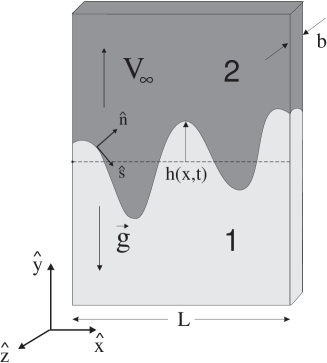
Let us first consider the Hele–Shaw problem in the channel geometry. We consider fluid 1 (viscosity $\mu_{1}$, density $\rho_{1}$) below fluid 2 ($\mu_{2},\rho_{2}$) (Fig. 1). The $\hat{z}$ axis is perpendicular to the cell. A velocity $V_{\infty}$ is imposed at infinity in the $\hat{y}$ direction. Gravity points from fluid 2 to fluid 1. The width of the cell is $L$, the gap between plates is $b$, and the surface tension between the fluids is $\sigma$.

The equations of motion for the interface and the boundary conditions are well known [7]. Here we will use the formulation of Tryggvason and Aref [11]. We introduce the velocity $\vec{U}=(\vec{u}_{1}+\vec{u}_{2})/2$ as the mean of the two limiting values of the velocities from both sides of the interface ($\vec{u}_{1},\vec{u}_{2}$) at a given point. This velocity $\vec{U}$ can be expressed in terms of the vortex sheet distribution $\gamma$ at the interface as:

$$\vec{U}(s,t)=\frac{1}{2\pi}P\int\frac{\hat{z}\times\left(\vec{r}(s,t)-\vec{r}(s^{\prime},t)\right)}{\mid\vec{r}(s,t)-\vec{r}(s^{\prime},t)\mid^{2}}\gamma(s^{\prime},t)ds^{\prime},$$ (1)

where:

$$\gamma=2A({\bf\hat{U}\cdot\hat{s}})+2C{\bf\hat{y}\cdot\hat{s}}+2D\kappa_{s},$$ (2)

with $s$ the arclength, $\kappa$ the curvature, and

$$A=\frac{\mu_{2}-\mu_{1}}{\mu_{2}+\mu_{1}},\ \ \ C=\frac{gb^{2}(\rho_{2}-\rho_{1})}{12(\mu_{2}+\mu_{1})}+AV_{\infty},\ \ \ D=\frac{\sigma b^{2}}{12(\mu_{2}+\mu_{1})},\ \ \ \gamma=(\vec{u}_{1}-\vec{u}_{2})\cdot\hat{s}.$$ (3)

For the purposes of this work it is convenient to rewrite these equations in terms of the interface height $h(x)$, following [38]. The equations read:

$$\vec{U}(x,t)=\frac{1}{2\pi}P\int_{-\infty}^{+\infty}\frac{(h(x^{\prime})-h(x),x-x^{\prime})}{(x-x^{\prime})^{2}+(h(x^{\prime})-h(x))^{2}}\tilde{\gamma}(x^{\prime})dx^{\prime},$$ (4)

$$\tilde{\gamma}=2D\kappa_{x}+2Ch_{x}+2A\vec{U}\cdot(1,h_{x}),$$ (5)

where:

$$\tilde{\gamma}=\gamma\sqrt{1+h_{x}^{2}},\qquad\kappa=\frac{h_{xx}}{(1+h_{x}^{2})^{3/2}}.$$ (6)

The dependence of $h$ and $\tilde{\gamma}$ on time is not written explicitly.

To complete the definition of the moving boundary problem the continuity of the normal velocity at the interface is required. This means that the velocity in the $y$ direction, $dh/dt$, projected along the normal direction, is equal to the normal component of the average velocity of the interface, $\vec{U}\cdot\hat{n}$:

$$\frac{dh}{dt}=U_{\hat{y}}-U_{\hat{x}}h_{x}.$$ (7)

In Section III we will consider the interface in the comoving frame ($\overline{h}=0$) and will look for the equation of evolution of $h(x,t)$.

B Radial geometry

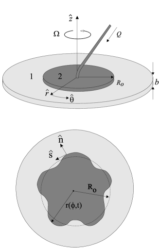
We proceed to write the corresponding equations for a circular cell rotating with angular velocity $\Omega$. The initial condition is $R=R_{0}$ (constant) and we label the outer (inner) fluid as the fluid 1 (2) which have known viscosities $\mu_{1}$, $\mu_{2}$ and densities $\rho_{1}$, $\rho_{2}$ (Fig. 2).

If we perform a change to polar coordinates in (1), and from arclength $s$ to angle $\phi$, we get for the mean velocity:

$$U_{\hat{r}}=\vec{U}(\phi_{1},t)\cdot\hat{r}=\frac{1}{2\pi}P\int_{0}^{2\pi}\frac{r_{2}^{2}\sin(\phi_{2}-\phi_{1})}{r_{1}^{2}+r_{2}^{2}-2r_{1}r_{2}\cos(\phi_{2}-\phi_{1})}\tilde{\gamma}(\phi_{2})d\phi_{2},$$ (8)

$$U_{\hat{\phi}}=\vec{U}(\phi_{1},t)\cdot\hat{\phi}=\frac{1}{2\pi}P\int_{0}^{2\pi}\frac{r_{1}r_{2}-r_{2}^{2}\cos(\phi_{2}-\phi_{1})}{r_{1}^{2}+r_{2}^{2}-2r_{1}r_{2}\cos(\phi_{2}-\phi_{1})}\tilde{\gamma}(\phi_{2})d\phi_{2},$$ (9)

where $\tilde{\gamma}=\sqrt{1+(r_{\phi}/r)^{2}}(\vec{u}_{1}-\vec{u}_{2})\cdot\hat{s}$, and we have used the notation $r(\phi_{1},t)\equiv r_{1}$, $r(\phi_{2},t)\equiv r_{2}$.

In the presence of sinks or sources the velocities $\vec{u}_{1}$ and $\vec{u}_{2}$ which define $\vec{U}$ include only the solenoidal part of the total velocity field. For this reason, in the presence of injection ($Q>0$) or withdrawal ($Q<0$) of the inner fluid, Eqs. (8) and (9) must be supplemented with the corresponding irrotational part of the velocity field.

In order to obtain the expression for the vorticity as a function of $\vec{u}_{i}$, we use the local equations known for this problem [27, 31]:

$$\vec{\nabla}p_{i}=-\frac{12\mu_{i}}{b^{2}}\left(\vec{u}_{i}+\frac{Q}{2\pi r}\hat{r}\right)+\Omega^{2}\rho_{i}r\hat{r},\qquad i=1,2$$ (10)

and the boundary conditions:

$$p_{2}-p_{1}=\sigma\kappa,\qquad\qquad u_{\hat{n}}^{(1)}=u_{\hat{n}}^{(2)}.$$ (11)

After some algebra, we can write an expression for the vorticity as a function of $\vec{U}$:

$$\tilde{\gamma}=\frac{b^{2}}{12}\frac{2\sigma}{r(\mu_{1}+\mu_{2})}\kappa_{\phi}+2A\vec{U}\cdot(\frac{r_{\phi}}{r},1)+2A\frac{Q}{2\pi r^{2}}r_{\phi}-\frac{b^{2}}{12}\frac{2\Omega^{2}(\rho_{2}-\rho_{1})}{\mu_{1}+\mu_{2}}r_{\phi},$$ (12)

with

$$\kappa=\frac{(r^{2}+2r_{\phi}^{2}-rr_{\phi\phi})}{(r^{2}+r_{\phi}^{2})^{\frac{3}{2}}},\qquad A=\frac{\mu_{2}-\mu_{1}}{\mu_{1}+\mu_{2}}.$$ (13)

The last step is to derive the equation of the continuity of the normal velocity. Now the projection of the radial velocity along the normal direction $\hat{n}$ has two contributions: the solenoidal part of the average velocity, $\vec{U}$, projected along $\hat{n}$, and the irrotational part of the mean interface velocity, $\vec{U}_{irrot}$:

$$\frac{dr}{dt}\hat{r}\cdot\hat{n}=\vec{U}\cdot\hat{n}+\vec{U}_{irrot}\cdot\hat{n}\ \ \rightarrow\ \ \frac{dr}{dt}=U_{\hat{r}}-\frac{r_{\phi}}{r}U_{\hat{\phi}}+\frac{Q}{2\pi r}.$$ (14)

This completes the system of equations for the two geometries considered. For an interface with no overhangs, Eqs. (4), (5), and (7) are the starting point for the generalized weakly nonlinear analysis in the rectangular cell. Equations (8), (9), (12), and (14) play the same role for the analysis in the rotating circular cell.

III Systematic weakly nonlinear analysis. Channel geometry

Our goal in this section is to introduce a systematic method to derive an evolution equation of the interface in real space to a given order in nonlinear couplings, in the channel geometry. The different orders of mode couplings will be ordered as powers of a “book–keeping” parameter $\varepsilon$, to be defined below. The evolution of the interface will thus take the form:

$$\frac{dh}{dt}=F[h]+\varepsilon G[h]+\varepsilon^{2}I[h]+\ldots,$$ (15)

where $F[h],G[h],\ldots$ are nonlocal operators on the function $h(x,t)$, including nonlinearities of order $n+1$ in the term of order $\varepsilon^{n}$. The small parameter $\varepsilon$ is defined as the ratio of two lengths, $\varepsilon=w/L$. We take $w$ as a measure of the characteristic scale of variation of the interface $h(x)$, while $L$ is either the width of the cell or, alternatively, the characteristic scale of variation in the $x$ direction. The weakly nonlinear regime is defined by the condition $w\ll L$.

The order $\varepsilon^{0}$ in Eq. (15) corresponds to the linearized equation. The order $\varepsilon^{1}$, when written in Fourier space, corresponds to the result of Miranda and Widom [29]. Here we will perform the explicit calculation to one order higher in $\varepsilon$ (up to $I[h]$) which is the leading nonlinear contribution in several important cases, such as the one discussed in Section III D. The systematics is presented in the channel geometry for simplicity.

A Dimensionless equations, expansion and convergence

We scale the interface height with $w$, the coordinate $x$ with $L$, and the time with $L/C$, where the velocity $C$ has been defined in (3).

The equations (4), (5), (6), and (7) become:

$$\vec{U}(x,t)=\frac{1}{2\pi}P\int_{-\infty}^{+\infty}\frac{(\varepsilon\left[h(x^{\prime})-h(x)\right],x-x^{\prime})}{(x-x^{\prime})^{2}\left\{1+\varepsilon^{2}\left[\frac{h(x^{\prime})-h(x)}{x^{\prime}-x}\right]^{2}\right\}}\tilde{\gamma}(x^{\prime})dx^{\prime},$$ (16)

$$\tilde{\gamma}=2B\kappa_{x}+2\varepsilon h_{x}+2A\vec{U}\cdot(1,\varepsilon h_{x}),$$ (17)

where

$$B=\frac{\sigma b^{2}}{12CL^{2}(\mu_{1}+\mu_{2})},\ \ \ \kappa=\frac{\varepsilon h_{xx}}{(1+\varepsilon^{2}h_{x}^{2})^{3/2}},$$ (18)

and

$$\frac{dh}{dt}=\frac{1}{\varepsilon}U_{\hat{y}}-U_{\hat{x}}h_{x}.$$ (19)

The starting point of our approach is an expansion of $\vec{U}$, $\tilde{\gamma}$ and $\kappa$ in powers of $\varepsilon$. Notice that the term $\left[h(x^{\prime})-h(x)\right]^{2}\ \left[x^{\prime}-x\right]^{2}$ between curly brackets in (16) is bounded provided that $h_{x}$ does not diverge. Equation (19) thus takes the form:

$$\frac{dh}{dt}=\frac{1}{\varepsilon}U_{\hat{y}}^{(0)}+U_{\hat{y}}^{(1)}-h_{x}U_{\hat{x}}^{(0)}+\varepsilon(U_{\hat{y}}^{(2)}-h_{x}U_{\hat{x}}^{(1)})+\cdots,$$ (20)

Before pursuing the calculation in detail, let us point out that the $\varepsilon$–expansion in Eq.(20) has a finite radius of convergence. This is guaranteed by the properties of uniform convergence of both the expansion of the denominator in Eq.(16) and the curvature. These properties allow us to commute the expansion with the integral in Eq.(16) and yield a convergent series of the form (20). The radius of convergence of the expansion of the denominator of Eq.(16) is given by the condition $\varepsilon^{2}\left[h(x^{\prime})-h(x)\right]^{2}\ \left[x^{\prime}-x\right]^{2}<1$, while the convergence of the curvature expansion is assured by the condition $\varepsilon^{2}h^{2}_{x}<1$. In the nonscaled original variables, the two conditions for convergence coincide, and read $MAX(|h_{x}|)<1$. If $|h_{x}|<1$ in the whole domain of integration, then the $\varepsilon$–expansion converges. If the condition is not fulfilled in some intervals, then Eq.(20) is an asymptotic expansion. Even in this case, the expansion contains useful information about the original problem.

An interesting case is $A=0$ which makes the vorticity independent of $\vec{U}$ in Eq.(16), so that Eq.(19) becomes a closed equation for $h(x,t)$. Then, in Eq.(20) it is easy to show that $U_{\hat{y}}^{(n)}=0$ when $n$ is even and $U_{\hat{x}}^{(n)}=0$ when $n$ is odd, a property that makes the even power terms of the expansion in Eq.(20) to vanish.

B First and second order expansion ($\varepsilon^{0}$ and $\varepsilon^{1}$)

Following the scheme introduced in the previous section we obtain from Eq.(16) that:

$$U_{\hat{x}}^{(0)}=0,\qquad U_{\hat{x}}^{(1)}=\frac{1}{2\pi}P\int_{-\infty}^{+\infty}\frac{h(x^{\prime})-h(x)}{(x-x^{\prime})^{2}}\tilde{\gamma}^{(0)}(x^{\prime})dx^{\prime},$$ (21)

$$U_{\hat{y}}^{(0)}=\frac{1}{2\pi}P\int_{-\infty}^{+\infty}\frac{\tilde{\gamma}^{(0)}(x^{\prime})}{x-x^{\prime}}dx^{\prime},\qquad U_{\hat{y}}^{(1)}=\frac{1}{2\pi}P\int_{-\infty}^{+\infty}\frac{\tilde{\gamma}^{(1)}(x^{\prime})}{x-x^{\prime}}dx^{\prime}.$$ (22)

Since $\tilde{\gamma}^{(0)}=2B\kappa_{x}^{(0)}+2AU_{\hat{x}}^{(0)}=0$ we get $U_{\hat{x}}^{(1)}=U_{\hat{y}}^{(0)}=0$. With this result we can study the first order term in the vorticity equation:

$$\tilde{\gamma}^{(1)}(x)=2B\kappa_{x}^{(1)}+2h_{x}+2AU_{\hat{x}}^{(1)}+2Ah_{x}U_{\hat{y}}^{(0)}.$$ (23)

Taking into account the definition of the Hilbert Transform:

$$H[f(x^{\prime})]=\frac{1}{\pi}P\int_{-\infty}^{+\infty}\frac{f(x^{\prime})}{x^{\prime}-x}dx^{\prime},$$ (24)

Eq.(20) up to order $\varepsilon^{0}$ reads:

$$\frac{dh}{dt}=-H[Bh_{x^{\prime}x^{\prime}x^{\prime}}+h_{x^{\prime}}].$$ (25)

The linear operator $F[h]$ in Eq.(15) thus reads explicitly:

$$F[h]=\frac{1}{\pi}P\int_{-\infty}^{+\infty}\frac{\left(h+Bh_{x^{\prime}x^{\prime}}\right)_{x^{\prime}}}{x-x^{\prime}}dx^{\prime}.$$ (26)

Writing $h(x,t)$ as a superposition of Fourier modes in Eq.(25) we recover the linear dispersion relation:

$$\frac{\dot{\delta}_{k}(t)}{\delta_{k}(t)}=\lambda(k)=\mid k\mid(1-Bk^{2}).$$ (27)

We will take $k$ as an integer but we should keep in mind that, upon restoring dimensions, $k$ should become $(2\pi/L)n$, with $n$ integer.

Let us pursue the systematics of the method by computing the next order in $\varepsilon$ in Eq.(19):

$$\frac{dh}{dt}=U_{\hat{y}}^{(1)}+\varepsilon U_{\hat{y}}^{(2)}=F[h]+\varepsilon G[h].$$ (28)

The computation of $U_{\hat{y}}^{(2)}$ requires an expression of the vorticity up to second order. This includes the evaluation of $U_{\hat{x}}^{(2)}$, which must be computed from the first order term of the vorticity. We get:

$$U_{\hat{x}}^{(2)}=H\left[\left(h(x^{\prime})f(x^{\prime})\right)_{x^{\prime}}\right]-h(x)H[f_{x^{\prime}}(x^{\prime})],$$ (29)

with $f(x)\equiv(Bh_{xx}+h)_{x}=\tilde{\gamma}^{(1)}(x)/2$, and:

$$U_{\hat{y}}^{(2)}=A\left\{H\left[h_{x^{\prime}}H[f(x^{\prime\prime})]\right]+H\left[h(x^{\prime})H[f_{x^{\prime\prime}}(x^{\prime\prime})]\right]+(hf)_{x}\right\}.$$ (30)

Taking the Fourier transform, we obtain:

$$\dot{\delta}_{k}=\lambda(k)\delta_{k}+\varepsilon A\mid k\mid\sum_{s=-\infty}^{+\infty}\left[1-\mbox{sgn}(ks)\right]\lambda(s)\delta_{s}(t)\delta_{k-s}(t),$$ (31)

which coincides with the result of Miranda and Widom in Ref. [29].

C Third order expansion ($\varepsilon^{2}$)

The expansion to order $\varepsilon^{2}$ is necessary to account for the lowest order nonlinearities in the case of zero viscosity contrast, and for other relevant situations such as the time dependent Saffman–Taylor finger solutions (section III D). We now have:

$$\frac{dh}{dt}={\cal{O}}(\varepsilon^{0})+{\cal{O}}(\varepsilon^{1})+\varepsilon^{2}(U_{\hat{y}}^{(3)}-h_{x}U_{\hat{x}}^{(2)})+\cdots$$ (32)

We have already computed $U_{\hat{x}}^{(2)}$ in Eq. (29). On the other hand:

$$U_{\hat{y}}^{(3)}=-\frac{1}{2}H[\tilde{\gamma}^{(3)}(x^{\prime})]+\frac{1}{2\pi}P\int_{-\infty}^{+\infty}\frac{\left[h(x^{\prime})-h(x)\right]^{2}}{(x^{\prime}-x)^{3}}\tilde{\gamma}^{(1)}(x^{\prime})dx^{\prime}.$$ (33)

Integrating twice by parts, the last integral can also be written as a Hilbert Transform. After some algebra we obtain the explicit form of the operator $I[h]$ containing the cubic nonlinearities in Eq.(15), which reads:

$$\begin{array}[]{ll}I[h]=&\frac{3}{2}H[g(x^{\prime})]+\frac{1}{2}H\left[\left(f(x^{\prime})[h(x)-h(x^{\prime})]^{2}\right)_{x^{\prime}x^{\prime}}\right]\\ &-h_{x}H\left[\left(f(x^{\prime})[h(x^{\prime})-h(x)]\right)_{x^{\prime}}\right]+V[h,A]\end{array}$$ (36)

with:

$$V[h,A]=A^{2}H\left[h(x^{\prime})H[\tau_{x^{\prime\prime}}(x^{\prime\prime})]+h_{x^{\prime}}(x^{\prime})H[\tau(x^{\prime\prime})]\right]+A^{2}(h\tau)_{x},$$ (37)

and:

$$g(x)=B\left(h_{xx}h_{x}^{2}\right)_{x},\qquad\tau(x)=U_{\hat{x}}^{(2)}+h_{x}U_{\hat{y}}^{(1)}=\frac{\tilde{\gamma}^{(2)}(x)}{2A}.$$ (38)

The same result in Fourier space takes the form:

$$\dot{\delta}_{k}(t)={\cal{O}}(1,\varepsilon)+\varepsilon^{2}\sum_{s,l=-\infty}^{+\infty}\delta_{l}\delta_{s-l}\delta_{k-s}\left[A^{2}T(k,s,l)-\frac{3}{2}BY(k,s,l)+W(k,s,l)\right],$$ (39)

with:

$$T(k,s,l)=\mid k\mid\mid s\mid\lambda(l)\left[1-\mbox{sgn}(ks)\right]\left[1-\mbox{sgn}(ls)\right],$$ (40)

$$Y(k,s,l)=\mid k\mid l^{2}(s-l)(k-s),$$ (41)

$$W(k,s,l)=\left[l\left(\frac{l}{2}+k-s\right)-sk\mbox{ sgn}(ls)+\frac{k^{2}}{2}\mbox{ sgn}(kl)\right]\lambda(l).$$ (42)

It is clear that the viscosity contrast in Eq.(39) appears squared because of the reflection symmetry (the simultaneous change $A\rightarrow-A$ and $h\rightarrow-h$ is a dynamical symmetry of the problem). Symmetry reasons alone, however, do not allow to discard a three mode coupling contribution when $A=0$. We see from our calculation that a three mode coupling is indeed present independently of $A$.

Following this scheme, the fourth order will carry a contribution proportional to $A$, and another proportional to $A^{3}$, for symmetry reasons. The fifth order will carry a contribution independent of $A$ and two others, proportional to $A^{2}$ and $A^{4}$, respectively. This scheme will continue for subsequent orders.

D Analysis of the time dependent single finger solution

In this section we perform a detailed analysis of the weakly nonlinear expansion in cases where exact solutions are known, namely single finger configurations with $B=0$. This allows to study how exact properties of solutions show up at the different orders, particularly concerning the role of viscosity contrast $A$.

At this point it is worth recalling that the case $A=1$ allows for a continuum of Saffman–Taylor finger solutions corresponding to different finger widths. A continuum of time dependent exact solutions, leading to those stationary states, is also known for $A=1$. However, for $A\neq 1$ only the one of width $\lambda=\frac{1}{2}$ remains a solution, $\lambda$ being the ratio of the finger width to the width of the channel. This result, which has been recently addressed in Ref.[26] although it was first discovered in Ref.[25], points out an intriguing connection between the width selection problem and the dynamical role of viscosity contrast. Here we will analyze the interplay between $A$ and $\lambda$ in the early nonlinear regime, and elucidate at what stage of the nonlinear dynamics does the viscosity contrast $A\neq 1$ prevents the possibility of having $\lambda\neq 1/2$.

From now on we consider $L=2\pi$, $B=0$, $C=1$, and we take as scaling velocity $(1-\lambda)C=(1-\lambda)\equiv\frac{\eta}{2}$. Conformal mapping techniques enable us to write the single finger solution of this problem in the form [25, 26]:

$$f(w,t)=-\ln w+d(t)+\eta\ln(1-\alpha(t)w),$$ (43)

where $f(w,t)=y+ix$, is an analytic function inside the unit disk in the $w$–complex plane, which maps that disk into the physical region occupied by the more viscous fluid. The interface is obtained in a parametric form by setting $w=e^{i\theta}$. The functions $\alpha(t)$, $d(t)$ verify:

$$\dot{d}(t)=\frac{\eta}{2-\eta}\left(\frac{\eta}{2}-\frac{\dot{\alpha}(t)}{\alpha(t)}\right),$$ (44)

$$\frac{\dot{\alpha}(t)}{\alpha(t)}=\frac{\eta}{2+\eta(\eta-2)+\eta(2-\eta)\frac{1+\alpha^{2}(t)}{1-\alpha^{2}(t)}}.$$ (45)

To obtain an expression for $h(x)$ in the weakly nonlinear regime of the evolution, $\alpha(t)$ and $d(t)$ are expanded in powers of a small parameter $\nu$:

$$d(t)=d^{(0)}(t)+\nu d^{(1)}(t)+\nu^{2}d^{(2)}(t)+\cdots\ \ ,\qquad\alpha(t)=\nu\alpha^{(0)}(t)+\nu^{2}\alpha^{(1)}(t).$$ (46)

Introducing these expansions in Eqs.(44) and (45) we obtain:

$$\dot{d}^{(0)}=\dot{d}^{(1)}=0,\qquad\dot{d}^{(2)}=\frac{\eta^{3}}{2}(\alpha^{(0)})^{2}(t),\qquad\dot{d}^{(3)}=\eta^{3}\alpha^{(0)}\alpha^{(1)},\ \ \cdots$$ (47)

$$\dot{\alpha}^{(0)}=\frac{\eta}{2}\alpha^{(0)},\qquad\dot{\alpha}^{(1)}=\frac{\eta}{2}\alpha^{(1)},\qquad\dot{\alpha}^{(2)}=\frac{\eta}{2}\left(\alpha^{(2)}-\eta(2-\eta)(\alpha^{(0)})^{3}\right),\ \ \cdots$$ (48)

which will be useful later. From (43) and (44) we obtain:

$$\begin{array}[]{ll}y=h=&-\nu\eta\alpha^{(0)}\cos\theta-\nu^{2}\left(\eta\alpha^{(1)}\cos\theta+\frac{\eta}{2}(\alpha^{(0)})^{2}\cos 2\theta-d^{(2)}\right)\\ &-\nu^{3}\left(\eta\alpha^{(2)}\cos\theta+\eta\alpha^{(0)}\alpha^{(1)}\cos 2\theta+\frac{\eta}{3}(\alpha^{(0)})^{3}\cos 3\theta-d^{(3)}\right)+{\rm\cal{O}}(\nu^{4}),\end{array}$$ (51)

$$x=-\theta-\nu\eta\alpha^{(0)}\sin\theta-\nu^{2}\left(\eta\alpha^{(1)}\sin\theta+\frac{\eta}{2}(\alpha^{(0)})^{2}\sin 2\theta\right)+{\rm\cal{O}}(\nu^{3}).$$ (52)

This last equation can be inverted in a systematic way to get:

$$\theta=-x+\nu\eta\alpha^{(0)}\sin x+\nu^{2}\left(\eta\alpha^{(1)}\sin x+\frac{\eta}{2}(1-\eta)(\alpha^{(0)})^{2}\sin 2x\right)+{\rm\cal{O}}(\nu^{3}).$$ (53)

The relation between $\theta$ and $x$ can be inverted in Eq.(51) and the cosine functions expanded. We obtain in this way the following expression for $h(x,t)$:

$$\begin{array}[]{ll}h(x,t)=&-\nu\eta\alpha^{(0)}\cos x-\nu^{2}\eta\left(\alpha^{(1)}\cos x+\frac{1-\eta}{2}(\alpha^{(0)})^{2}\cos 2x\right)+\\ &\nu^{3}\eta\left\{(\eta-1)\alpha^{(0)}\alpha^{(1)}\cos 2x+\left(\frac{3\eta}{8}(\eta-2)(\alpha^{(0)})^{3}-\alpha^{(2)}\right)\cos x+\right.\\ &\left.\left(\frac{3\eta}{8}(2-\eta)-\frac{1}{3}\right)(\alpha^{(0)})^{3}\cos 3x\right\}+{\rm\cal{O}}(\nu^{4}).\end{array}$$ (57)

In order to follow the scheme developed in the previous section, we must measure $h(x,t)$ in units of its characteristic amplitude $\nu$. In this way, the previous equation (57) takes the form:

$$h=h^{(0)}+\nu h^{(1)}+\nu^{2}h^{(2)}+{\rm\cal{O}}(\nu^{3}),$$ (58)

where $h(x,t)$ represents now $h(x,t)/\nu$, and the small parameter $\nu$ is directly comparable to the small parameter $\varepsilon$ of the previous section. The expression for $h(x,t)$ can be regarded as a series of modes of decreasing amplitude in our expansion (15) (written in the units of this problem), and matching the corresponding powers in either $\varepsilon$ or $\nu$ we obtain:

$$\frac{dh^{(0)}}{dt}=\frac{\eta}{2}F[h^{(0)}]$$ (59)

to order $\varepsilon^{0}$.

This identity can be verified (independently of $A$) by substituting the expression of $h^{(0)}$ and using Eqs.(48) and (25) for the left and right hand side respectively. At order $\varepsilon$ we have:

$$\frac{dh^{(1)}}{dt}=\frac{\eta}{2}\left(F[h^{(1)}]+G[h^{(0)},h^{(0)}]\right).$$ (60)

The second term of the right hand side gives no contribution, and we obtain an interesting result: the equation at order $\varepsilon$ is verified independently of $\eta$ and $A$. Hence, we cannot establish the difference between $A=1$ (compatible with any $\eta$) and $A\neq 1$ (compatible only with $\eta=1$) at this order.

The difference between these two situations arises at order $\varepsilon^{2}$:

$$\frac{dh^{(2)}}{dt}=\frac{\eta}{2}\left(F[h^{(2)}]+G[h^{(0)},h^{(1)}]+L[h^{(0)},h^{(0)},h^{(0)}]\right).$$ (61)

Since the left hand side of the equation involves only the modes $\cos x$, $\cos 2x$, and $\cos 3x$, the right hand side of the equation must include these same modes with the same coefficients. The coefficients for $\cos 2x$ and $\cos 3x$ are easily matched. For $\cos x$ the left hand side reads:

$$\left(\frac{\eta^{3}(\eta-2)}{16}(\alpha^{(0)})^{3}-\frac{\eta^{2}}{2}\alpha^{(2)}\right)\cos x,$$ (62)

where we have used Eq. (48), and the right hand side reads:

$$\left(\frac{3\eta^{3}(\eta-2)}{16}(\alpha^{(0)})^{3}-\frac{\eta^{2}}{2}\alpha^{(2)}\right)\cos x+A\frac{\eta^{3}(1-\eta)}{4}(\alpha^{(0)})^{3}\cos x+\frac{\eta^{4}}{8}(\alpha^{(0)})^{3}\cos x.$$ (63)

Hence, the requirement for matching the coefficients on both sides is:

$$\frac{\eta^{3}}{4}(1-\eta)=A\frac{\eta^{3}}{4}(1-\eta),$$ (64)

which is always true if $\eta=1$ ($\lambda=1/2$), but for $\eta\neq 1$ ($\lambda\neq 1/2$) it requires $A=1$. This result shows that the nontrivial relationship between $A$ and $\lambda$ which is known from exact solutions is already manifest at the early nonlinear stages of the dynamics. This clearly illustrates the potential usefulness of the weakly nonlinear expansion at a purely analytical level, in that a dynamical property of the problem which must be satisfied at all orders (in this case the incompatibility of $A\neq 1$ and $\lambda\neq 1/2$) may be detected at a low order in the expansion, without having to know the exact solution to all orders.

If we pursue the expansion to higher orders, the general expression for $h^{(n)}$ takes the form:

$$h^{(n)}=\sum_{k=1}^{n+1}\beta_{k}^{(n)}(t)\cos(kx),$$ (65)

where each coefficient is a function of $\alpha(t)$. The even modes of the solution with $\eta=1$ have zero coefficients because they must remain invariant under a change of sign and translation by $\pi$.

So far in this section we have restricted ourselves to $B=0$ in order to compare with exact results. However, we can carry out the analysis also for $B\neq 0$. It can be shown that the structure of the expression (65) is preserved in this case. The coefficients $\beta_{k}^{(n)}(t)$ are obtained as solutions of a set of differential equations which contain the surface tension $B$. For instance, to third order we have:

$$h(x,t)=\left(\beta_{1}^{(0)}+\varepsilon\beta_{1}^{(1)}+\varepsilon^{2}\beta_{1}^{(2)}\right)\cos x+\left(\varepsilon\beta_{2}^{(1)}+\varepsilon^{2}\beta_{2}^{(2)}\right)\cos 2x+\varepsilon^{2}\beta_{3}^{(2)}\cos 3x,$$ (66)

which, introduced in Eq.(15), leads to the following equations:

$$\begin{array}[]{c}\dot{\beta}_{1}^{(0)}=V_{0}(1-B)\beta_{1}^{(0)},\qquad\dot{\beta}_{1}^{(1)}=V_{0}(1-B)\beta_{1}^{(1)},\qquad\dot{\beta}_{2}^{(1)}=2V_{0}(1-4B)\beta_{2}^{(1)},\\ \displaystyle{\dot{\beta}_{2}^{(2)}=2V_{0}(1-4B)\beta_{2}^{(2)},\qquad\dot{\beta}_{3}^{(2)}=3V_{0}(1-9B)\beta_{3}^{(2)}-\frac{9BV_{0}}{8}(\beta_{1}^{(0)})^{3},}\\ \displaystyle{\dot{\beta}_{1}^{(2)}=V_{0}(1-B)\beta_{1}^{(2)}+AV_{0}(1-B)\beta_{2}^{(1)}\beta_{1}^{(0)}-\frac{V_{0}}{8}(2-5B)(\beta_{1}^{(0)})^{3},}\end{array}$$ (70)

once the dimensions are reintroduced. In this way we can also see how surface tension perturbs the dynamics at the weakly nonlinear regime. Clearly, at these early stages of the nonlinear evolution there is no sign of the singular perturbation character of surface tension, which, at the late stages of the evolution will be responsible for the selection of the steady state[1].

IV Application of the method to the rotating Hele–Shaw cell

A Dimensionless equations in the radial geometry

The $\varepsilon$ expansion in the channel geometry originated in the different scaling of lengths in the $x$ and $y$ directions. To perform an equivalent expansion in the radial geometry we first split the function $r(\phi,t)$ in two parts, namely the radius of the unperturbed circle and the departure from this circle:

$$r(\phi,t)\qquad\rightarrow\qquad\sqrt{R_{0}^{2}+\frac{Qt}{\pi}}+r(\phi,t)=R(t)+r(\phi,t).$$ (71)

The largest length scale in the problem is given by $R(t)$, which is only a constant in the absence of injection. For finite injection rate, $R(t)$ defines an evolving (unstable) solution. The proper scaling of $r(\phi,t)$, which will define the weakly nonlinear dynamics now, is not the naive extension of the scaling defined in the channel geometry (namely $\varepsilon=w/R$, $w$ being the typical departure from circularity). In fact, this scaling would mix different orders of the weakly nonlinear analysis. The reason for this was already pointed out by Miranda and Widom [30]: in the radial geometry, mass conservation implies that the zero mode (which in the channel geometry is decoupled from the rest and drops out of the formulation) has a higher order nonzero amplitude, since it must satisfy a mass conservation relation which, to lowest order, reads:

$$\delta_{0}=-\frac{1}{2R}\sum_{k\neq 0}\mid\delta_{k}\mid^{2}.$$ (72)

Following this observation, we split the deviation from $R$ in two terms, so that the radial function reads $r=R+\tilde{r}+r_{0}$, where $r_{0}$ represents the zero mode (an expansion or contraction of the circle), and $\tilde{r}$ the other modes. We scale them in the form $\tilde{r}\rightarrow w\tilde{r}$, $r_{0}\rightarrow(w^{2}/R)r_{0}$, and write the position of the interface $r(\phi)$ as:

$$r(\phi)\rightarrow R(1+\varepsilon r(\phi)),$$ (73)

where:

$$r(\phi)=\tilde{r}(\phi)+\varepsilon r_{0}.$$ (74)

To simplify the notation, we have dropped out the time dependence.

The velocities will be scaled by:

$$V_{0}=\frac{1}{\mu_{2}+\mu_{1}}\left(\frac{Q(\mu_{2}-\mu_{1})}{2\pi R}-\frac{b^{2}}{12}\Omega^{2}(\rho_{2}-\rho_{1})R\right),$$ (75)

implying that time will be scaled by $R/V_{0}$. Once equations (8), (9), (12), and (14) are made dimensionless, we have:

$$\tilde{\gamma}=2B\frac{\kappa_{\phi}}{1+\varepsilon r}+2A\vec{U}\cdot(\frac{\varepsilon r_{\phi}}{1+\varepsilon r},1)+2\varepsilon\left(\frac{C}{(1+\varepsilon r)^{2}}-D\right)r_{\phi},$$ (76)

for the vorticity, where:

$$\begin{array}[]{c}\displaystyle{B=\frac{b^{2}}{12}\frac{\sigma}{(\mu_{1}+\mu_{2})V_{0}R^{2}},\qquad C=\frac{QA}{2\pi RV_{0}},\qquad D=\frac{b^{2}}{12}\frac{\Omega^{2}\triangle\rho R}{(\mu_{1}+\mu_{2})V_{0}},\vspace{0.5cm}}\\ \displaystyle{\kappa=\frac{(1+\varepsilon r)^{2}+2\varepsilon^{2}r_{\phi}^{2}-\varepsilon(1+\varepsilon r)r_{\phi\phi}}{\left[(1+\varepsilon r)^{2}+\varepsilon^{2}r_{\phi}^{2}\right]^{\frac{3}{2}}},\qquad A=\frac{\mu_{2}-\mu_{1}}{\mu_{2}+\mu_{1}},\qquad\triangle\rho=\rho_{2}-\rho_{1}.}\end{array}$$ (79)

For the integrals:

$$U_{\hat{r}}(\phi)=\frac{1}{4\pi}P\int_{0}^{2\pi}\frac{1+2\varepsilon r_{2}+\varepsilon^{2}r_{2}^{2}}{\tan\left(\frac{\phi_{2}-\phi_{1}}{2}\right)\left[1+\varepsilon f(\phi_{1},\phi_{2})+\varepsilon^{2}g(\phi_{1},\phi_{2})\right]}\tilde{\gamma}(\phi_{2},t)d\phi_{2},$$ (80)

$$U_{\hat{\phi}}(\phi)=\frac{1}{4\pi}P\int_{0}^{2\pi}\frac{1+\varepsilon f(\phi_{1},\phi_{2})+\varepsilon^{2}r_{1}r_{2}-(1+2\varepsilon r_{2}+\varepsilon^{2}r_{2}^{2})\cos(\phi_{2}-\phi_{1})}{2\sin^{2}\left(\frac{\phi_{2}-\phi_{1}}{2}\right)\left[1+\varepsilon f(\phi_{1},\phi_{2})+\varepsilon^{2}g(\phi_{1},\phi_{2})\right]}\tilde{\gamma}(\phi_{2})d\phi_{2},$$ (81)

with:

$$f(\phi_{1},\phi_{2})=r_{1}+r_{2},\qquad g(\phi_{1},\phi_{2})=\frac{(r_{1}-r_{2})^{2}}{4\sin^{2}\left(\frac{\phi_{2}-\phi_{1}}{2}\right)}+r_{1}r_{2},$$ (82)

and for the evolution of the deviation from $R(t)$:

$$\varepsilon\frac{d\tilde{r}}{dt}+\varepsilon^{2}\frac{dr_{0}}{dt}=U_{\hat{r}}-\varepsilon\frac{r_{\phi}U_{\hat{\phi}}}{1+\varepsilon r}+\frac{Q}{2\pi RV_{0}}\left[\frac{1}{1+\varepsilon r}-(1-\varepsilon^{2}r_{0})\right].$$ (83)

Eq.(83) above is the only one which is sensitive to the different possible scalings of the deviation from circularity, due to the time derivatives. The choice we propose is the only one which is truly systematic. Other possibilities are not incorrect but will mix different orders of the weakly nonlinear expansion at a given order in $\varepsilon$.

B The linear dispersion relation

Our goal now is to obtain the linear dispersion relation and the leading weakly nonlinear corrections, in both real and Fourier space, and to discuss the interplay between rotation and injection at the early stages of the instability.

We will use the following definitions for the average of a function and for the Hilbert transform in the unit circle:

$$\overline{f}=\frac{1}{2\pi}\int_{0}^{2\pi}f(\phi)d\phi,\qquad H[f(\phi^{\prime})]=\frac{1}{2\pi}P\int_{0}^{2\pi}f(\phi^{\prime})\cot\left(\frac{\phi^{\prime}-\phi}{2}\right)d\phi^{\prime}.$$ (84)

The zero order of the vorticity and the two components of the velocity are:

$$\tilde{\gamma}^{(0)}=2AU_{\hat{\phi}}^{(0)},\qquad U_{\hat{\phi}}^{(0)}=\frac{\overline{\tilde{\gamma}^{(0)}}}{2},\qquad U_{\hat{r}}^{(0)}=\frac{1}{2}H[\tilde{\gamma}^{(0)}(\phi^{\prime})],$$ (85)

and thus:

$$\tilde{\gamma}^{(0)}=A\overline{\tilde{\gamma}^{0}}.$$ (86)

This is different from its counterpart in the channel geometry. Here the equations for the vorticity at consecutive orders require the knowledge of the average vorticity. The equations are solved by averaging on both sides. For example, at zero order, $A\neq 1$ will lead to $\tilde{\gamma}^{(0)}=0$, but for $A=1$, $\tilde{\gamma}^{(0)}$ can be any constant. The presence of an arbitrary constant is not a problem, since it is eliminated at each order in the equation for the evolution of the interface.

Expanding the equations up to first order, and using $\tilde{\gamma}^{(0)}=0$, the linearized equation for the evolution of the interface deviation reads:

$$\frac{d\tilde{r}}{dt}=U_{\hat{r}}^{(1)}-\frac{Q}{2\pi RV_{0}}\tilde{r}=\frac{1}{2}H[\tilde{\gamma}^{(1)}]-\frac{Q}{2\pi RV_{0}}\tilde{r},$$ (87)

with:

$$\tilde{\gamma}^{(1)}=-2B(\tilde{r}+\tilde{r}_{\phi\phi})_{\phi}+2(C-D)\tilde{r}_{\phi}.$$ (88)

We can now perform a Fourier transform of the equations and, after reintroducing the adequate dimensions, we find:

$$\lambda(n)=\left(\frac{b^{2}}{12}\frac{\Omega^{2}\triangle\rho}{\mu_{1}+\mu_{2}}-\frac{QA}{2\pi R^{2}}\right)\mid n\mid-\frac{b^{2}}{12R^{3}}\frac{\sigma}{\mu_{1}+\mu_{2}}\mid n\mid(n^{2}-1)-\frac{Q}{2\pi R^{2}}.$$ (89)

This is the linear dispersion relation found in [27].

We now return to the question of the different scaling alternatives introduced at the end of Section IV A. Had we used the scaling $\varepsilon=w/R^{2}(t)$, the term $Q/(2\pi R^{2})$ in (89) would have disappeared before reintroducing the dimensions. On the contrary, for $\varepsilon=w$ this term becomes multiplied by a factor $2$. These changes in the dimensionless linear dispersion relation come from the fact that a mode $\delta_{n}$ in the scaling adopted in (73) and (74) becomes $\delta_{n}/R$ in the first of the scaling alternatives above.

The term $Q/(2\pi R^{2})$ at the end of Eq. (89) is stabilizing for positive injection rate ($Q>0$) and destabilizing for $Q<0$. In a sense this is a purely geometric effect, which contributes to the growth or decay of modes due to the expansion or contraction of the base state. As pointed out in [36] the term $Q/(2\pi R^{2})$, which can be scaled out, must be distinguished from the rest, which do describe the intrinsic instability of the problem. Disregarding that last term, it is then clear that injection and rotation ($CV_{0}$ and $DV_{0}$ respectively) play an equivalent role in the linear dispersion relation, since both appear multiplying $n$. By choosing the proper viscosity and density contrasts, they can produce exactly the same stabilizing or destabilizing effect. This is the counterpart, in the radial geometry, of the equivalence between the roles of injection and gravity in the channel geometry. In the channel geometry, however, the equivalence is exact and can thus be extended to all the nonlinear evolution (in the appropriate reference frame). This is not the case in radial geometry, as shown in the next section.

C Weakly nonlinear theory with rotation

The purpose of this section is to derive the leading order nonlinear contributions for the general problem with both rotation and injection. We first recall that mass conservation related the zero mode to the other modes. In the original nonscaled variables this reads:

$$\dot{\delta}_{0}=-\frac{Q}{2\pi R^{2}}\delta_{0}-\frac{1}{R}\sum_{k\neq 0}\mid\delta_{k}\mid^{2}\lambda(k).$$ (90)

To reproduce this result and the nonlinear couplings for the other modes we start with the equation for the interface at order $\varepsilon^{2}$:

$$\frac{d\tilde{r}}{dt}+\varepsilon\frac{dr_{o}}{dt}={\rm\cal{O}}(\varepsilon^{0})+\varepsilon\left(U_{\hat{r}}^{(2)}+\frac{Q}{2\pi RV_{0}}\tilde{r}^{2}\right),$$ (91)

where we have used that $U_{\hat{\phi}}^{(1)}=U_{\hat{\phi}}^{(0)}=U_{\hat{r}}^{(0)}=\tilde{\gamma}^{(0)}=\overline{\tilde{\gamma}^{(0)}}=0$. The velocity $U_{\hat{r}}^{(2)}$ can be obtained from the expansion of $U_{\hat{r}}$:

$$U_{\hat{r}}^{(2)}=\frac{1}{2}H[\tilde{\gamma}^{(2)}(\phi^{\prime})]+\frac{1}{2}H[(\tilde{r}(\phi^{\prime})-\tilde{r}(\phi))\tilde{\gamma}^{(1)}(\phi^{\prime})],$$ (92)

where:

$$\tilde{\gamma}^{(2)}=2B\kappa^{(2)}-2B\tilde{r}\kappa^{(1)}+2A\tilde{r}_{\phi}U_{\hat{r}}^{(1)}+2AU_{\hat{\phi}}^{(2)}-4C\tilde{r}\tilde{r}_{\phi}.$$ (93)

$\kappa^{(2)}$ and $U_{\hat{\phi}}^{(2)}$ can be computed from (79) and (81) respectively. The latter involves only $\tilde{\gamma}^{(1)}$. We obtain finally:

$$\begin{array}[]{cc}\displaystyle{\frac{d\tilde{r}}{dt}+\varepsilon\frac{dr_{o}}{dt}={\rm\cal{O}}(\varepsilon^{0})+\varepsilon}&\left(H\left[B\kappa_{\phi^{\prime}}^{(2)}-\frac{C+D}{2}(\tilde{r}^{2})_{\phi^{\prime}}\right]+\tilde{r}H[s_{\phi^{\prime}}]+AH[H[(\tilde{r}s_{\phi^{\prime\prime}})_{\phi^{\prime\prime}}]]\right.\\ &-\left.AH\left[\tilde{r}(\phi^{\prime})H[s_{\phi^{\prime\prime}\phi^{\prime\prime}}]+\tilde{r}_{\phi^{\prime}}H[s_{\phi^{\prime\prime}}]\right]+\frac{Q}{2\pi RV_{0}}\tilde{r}^{2}\right),\end{array}$$ (96)

with:

$$\kappa^{(2)}=\tilde{r}^{2}+\frac{\tilde{r}_{\phi}^{2}}{2}+2\tilde{r}\tilde{r}_{\phi\phi},\qquad s_{\phi}=\left(B(\tilde{r}+\tilde{r}_{\phi\phi})+(D-C)\tilde{r}\right)_{\phi}.$$ (97)

By introducing a superposition of Fourier modes in $\tilde{r}$ we directly recover Eq.(90). For the other modes ($k\neq 0$) we get the result:

$$\dot{\delta}_{n}=\lambda(n)\delta_{n}+\sum_{k\neq 0,n}\delta_{k}\delta_{n-k}(F(k,n)+S(k,n)+\lambda(k)J(k,n)),$$ (98)

where:

$$F(k,n)=\frac{\mid n\mid}{R}\left[-\frac{QA}{2\pi R^{2}}\left(\frac{1}{2}-\mbox{sgn}(kn)\right)+\frac{b^{2}}{24}\frac{\Omega^{2}\triangle\rho}{\mu_{1}+\mu_{2}}\right],$$ (99)

$$S(k,n)=\frac{\mid n\mid}{R}\left[\frac{b^{2}}{12R^{3}}\frac{\sigma}{\mu_{1}+\mu_{2}}\left(1-\frac{k}{2}(n+3k)\right)\right],$$ (100)

$$J(k,n)=-\frac{1}{R}\left[A\mid n\mid(1-\mbox{ sgn}(kn))+1\right].$$ (101)

For the particular case $\Omega=0$, the expression above reproduces the result of Miranda and Widom [30]. We find that the presence of rotation does not change the formal structure of the equations, but introduces new terms.

To emphasize the roles of injection and rotation, we define the quantity $H(k,n)$ as the part of the coupling matrix in the r.h.s. of Eq.(98) which contains $Q$ and/or $\Omega$. This quantity reads:

$$H(k,n)=\frac{\mid n\mid}{2R}\left(\frac{QA}{2\pi R^{2}}+\frac{b^{2}}{12}\frac{\Omega^{2}\triangle\rho}{\mu_{1}+\mu_{2}}\right)+J(k,n)\mid k\mid\left(\frac{b^{2}}{12}\frac{\Omega^{2}\triangle\rho}{\mu_{1}+\mu_{2}}-\frac{QA}{2\pi R^{2}}\right)+\frac{Q}{2\pi R^{3}}.$$ (102)

We observe that experimental parameters occur only in two groups, namely:

$$\tilde{\Omega}=\frac{b^{2}}{12}\frac{\Omega^{2}\triangle\rho}{\mu_{1}+\mu_{2}},\qquad\tilde{Q}=\frac{QA}{2\pi R^{2}}.$$ (103)

Both of them turn out to multiply the same functions of the wave numbers, except for changes in sign. However, notice that the relative sign of $\tilde{\Omega}$ and $\tilde{Q}$ is different in the linear part and in the leading nonlinear part of the dynamics. This clearly shows that the effects of injection and rotation cannot be interchanged by simple changes in parameters, and that the intrinsic new dimensionless parameter related to rotation already shows up at the early nonlinear regime.

It is also remarkable that, for $Q\neq 0$, $R(t)$ is time dependent, and the relative weight of $\tilde{\Omega}$ and $\tilde{Q}$ changes with time. This may have remarkable consequences in the highly nonlinear regime. For instance, rotation can prevent the formation of finite time singularities in the case with zero surface tension [36].

Finally, notice that at nonlinear order there is also a geometrical term, $Q/(2\pi R^{3})$, independent of $n$. This term cannot be scaled out by the same procedure that eliminated its counterpart at linear order.

V Numerical study of an exact solution and its weakly nonlinear approximation

The purpose of this section is to put the weakly nonlinear analysis to the test, as a quantitative approximation. We will check it against an exact time dependent solution of the case $B=0$ which evolves towards the Saffman–Taylor finger of width $\lambda=1/2$ in the channel geometry. This will allow us to check how fast is the convergence of the expansion and how accurate it may be even beyond its radius of convergence, when it becomes an asymptotic series.

We define $F$ as the ratio between the maximum height of the interface (at the finger tip) and half the width of the cell (in our case $L=2\pi$). $F$ is a dimensionless amplitude which is proportional to $\varepsilon$ and thus measures how deep the system is into the nonlinear regime. Furhermore, since the system is described by the evolution of a curve, it may also be convenient to have a more global characterization of its configuration in order to compare the exact result and the different approximations. We propose the use of the flux $\Phi$, defined as the total amount of fluid 1 per unit length and unit time flowing across the horizontal line located at the mean interface position [18]).

A The time dependent exact solution with $B=0$ and $\lambda=1/2$

An explicit solution of the problem without surface tension ($B=0$) and valid for any viscosity contrast $A$, describing the growth of a single finger which asymptotically fills half of the channel ($\lambda=1/2$), can be obtained from Eqs.(43), (44), and (45). This reads:

$$f(w,t)=-\ln w+V_{o}t+a(0)+\ln\left[\sqrt{1+(b(0)^{2}-1)\exp(2V_{o}t)}+w\right],$$ (104)

with $a(0)$ and $b(0)$ as initial constants, and $b(0)\gg 1$. Since this solution is valid for any $A$, particularly $A=0$, all terms of the weakly nonlinear equation (15) depending on $A$ will necessarily have no contribution.

We will take the following values for the parameters:

$$V_{o}=\frac{1}{2},\qquad b(0)=\frac{1}{\nu}=1000,\qquad a(0)=\ln\nu+\frac{\nu^{2}}{2}.$$ (105)

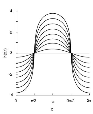
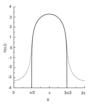
Fig. 3 shows the evolution of the interface for this solution. When $F\simeq 1$ the finger shape is indistinguishable from the stationary Saffman–Taylor solution (Fig. 4), except near the points $x=\pi/2$ and $x=3\pi/2$ when the asymptotes of the finger must develop at infinite time. When $F=1/\pi$, the slope of the interface becomes $1$ at these two points and the series (15) loses its convergence, according to the discussion of Section III A.

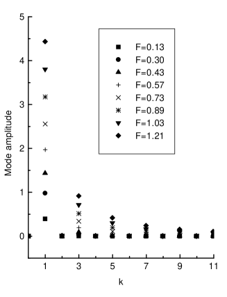
In Fig. 5 we present the amplitude of the Fourier modes of the exact solution. It is clear that relatively few modes suffice to accurately reproduce the stationary finger shape in the tip region.

B Expansion of the exact solution

In Section III D we expanded the exact solution (43) in a small parameter $\nu$. This expansion revealed a hierarchy of amplitudes of the different modes for an initial condition close to the planar interface. The solution (104) can be expanded similarly and yields:

$$\nu=\frac{1}{b(0)},\ \ \ \alpha(t)=-\frac{\nu}{b(t)},\ \ \ d(t)=V_{o}t+\ln b(t),\ \ \ b(t)=\sqrt{\nu^{2}+(1-\nu^{2})\exp(2V_{o}t)}.$$ (106)

In agreement with (57), and using the same parameters as in the previous section, we obtain up to third order:

$$h(x,t)=\nu e^{t/2}\cos x+\nu^{3}\left[\left(\frac{1}{2}e^{t/2}-\frac{1}{8}e^{3t/2}\right)\cos x-\frac{1}{24}e^{3t/2}\cos 3x\right].$$ (107)

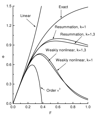
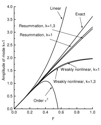
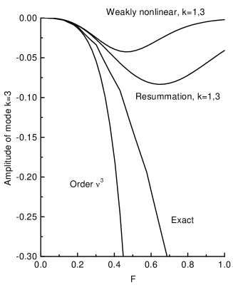
The exact flux $\Phi$ can be easily computed from the stream function, which in its turn can be related to the form of the mapping Eq.(104) (see for instance Ref.[18]). In Fig. 6 we compare the flux $\Phi$ of the approximate result above with the exact result coming from (104). We clearly observe that the first correction to the linear regime improves the flux (to a 5 % accuracy) from $F\simeq 0.12$ to $F\simeq 0.17$. The amplitude of the mode $k=1$ (Fig. 8) is fairly well reproduced by the linear approximation up to $F\simeq 0.20$, and the correction of order $\nu^{3}$ gives a value for the mode $k=3$ reasonably good up to $F\simeq 0.20$ (Fig. 9) and improves the mode $k=1$ almost until $F\simeq 0.25$. Above these values of $F$ the deviation from the exact interface is exponential.

Notice that the expansion up to $\nu^{3}$ considered here does not account for the complete three mode coupling of Eq.(39) which contains part of the higher orders in $\nu$. This explains why going from order $\nu$ (linear) to order $\nu^{3}$ improves only slightly the shape of the finger, the flux $\Phi$, and the amplitude of the mode $k=1$.

C Weakly nonlinear expansion

In this section we study the mode coupling equation (39). We solve this equation in cases where only modes $k=1$ and $k=1,3$ are present, and compare the result with both the exact solution and the approximation to order $\nu^{3}$ introduced in the two previous sections.

We consider the initial condition $\beta_{1}(0)=\varepsilon=0.001$ for the first mode and zero for the rest of modes. We use Eq. (39) recalling that, since $\beta_{i}$ represent the amplitudes of the cosine functions, $\delta_{i}=\beta_{i}/2$. The result is that the modes $k\neq 1$ remain zero and:

$$\beta_{1}(t)=\frac{\varepsilon\exp(0.5t)}{\sqrt{1+0.25\varepsilon^{2}(\exp(t)-1)}},$$ (108)

where we see that the mode $k=1$ saturates to a finite value as $t\to\infty$. Returning to Fig. 6 and 7, we see that the flux $\Phi$ approximates the exact value to a 5 % uncertainty) until $F\simeq 0.23$. Fig. 8 shows that the amplitude of the first mode starts deviating significantly from the exact solution around $F\simeq 0.40$.

Next, we add the third mode to the equation (39) with the initial condition $\beta_{1}=\varepsilon+3\varepsilon^{3}/8$ and $\beta_{3}=\varepsilon^{3}/24$. The set of equations to be solved numerically is:

$$\dot{\beta}_{1}=\frac{1}{2}\beta_{1}-\frac{1}{8}\beta_{1}^{3}-\frac{5}{4}\beta_{3}^{2}\beta_{1}+\frac{1}{4}\beta_{1}^{2}\beta_{3},$$ (109)

$$\dot{\beta}_{3}=\frac{3}{2}\beta_{3}-\frac{3}{4}\beta_{1}^{2}\beta_{3}-\frac{27}{8}\beta_{3}^{3}.$$ (110)

As shown in Figs. 6 and 9 the flux does not improve significantly, while the amplitude of the mode $k=3$ remains acceptable almost until $F\simeq 0.25$, and improves the previous result by more than a 50 % almost until $F\simeq 0.33$. Beyond this value of $F$ the third mode falls to zero due to the second term in the r.h.s. of Eq.(110), proportional to $\beta_{1}^{2}\beta_{3}$ but negative. This is a signature that higher order terms, for instance of order $\beta_{1}^{4}\beta_{3}$, become important when $\beta_{1}$ is of order one.

From this study we can conclude that using only two modes and the lowest order nonlinear correction for this case (involving three mode couplings), both the shape of the interface and the total flux are reasonably well described within the whole range of convergence of the series (up to $F\simeq 1/\pi$). This indicates that the weakly nonlinear description of the problem works remarkably well at the quantitative level, at least in some physically relevant cases. To what extent this conclusion holds for more complicated situations, for instance those involving competition of different fingers, remains an open question.

D Partial resummation

According to Eq. (39), we can write a closed equation for the mode $k=1$ which is correct up to third order couplings, of the form:

$$\dot{\beta}_{1}=\frac{1}{2}\beta_{1}-\frac{1}{4}\beta_{1}^{2}\dot{\beta}_{1},$$ (111)

where the mode $k=3$ has been set initially to zero.

The presence of $\dot{\beta}_{1}$ in the right hand side gives rise to terms of order higher than $\beta_{1}^{3}$. Thus, solving this equation amounts to doing a partial resummation of these higher order terms. This kind of closed differential equation was already obtained in Ref.[29]. In our approach this differential equation is obtained in a systematic way by identifying the terms $\lambda(n)\beta_{n}$ and replacing them for $\dot{\beta}_{n}$. For example, in Eq. (39) the term $T(k,s,l)$ could have been partially resummated in the two mode coupling differential equation.

The solution of Eq.(111) yields the transcendental form:

$$t=2\ln\left(\frac{\beta_{1}}{\varepsilon}\right)+\frac{1}{4}(\beta_{1}^{2}-\varepsilon^{2}).$$ (112)

A numerical computation of the flux based on this equation shows a dramatic improvement up to $F\simeq 1/\pi$. It is surprising and remarkable that the equation for a single mode, including the resummation suggested by the first nonlinear correction, reproduces the exact solution to a great accuracy in the full range of convergence and defines an excellent approximation further inside the nonlinear regime. This suggests that this kind of resummation is not arbitrary, and might have a deeper physical justification.

In addition, we obtain an amplitude for the mode $k=1$ within 10 % accuracy up to $F\simeq 0.8$, and it is still quite good until $F=1$. Although the exact spectrum shows the increasing importance of the mode $k=3$ at these values of $F$, the agreement between the exact result and this approximation for a single mode $k=1$ is quite remarkable.

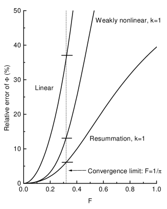
We recall that the series converges up to $F\simeq 1/\pi$. Beyond this value of $F$, increasing the order of mode coupling in Eq. (111) does not guarantee that the approximation improves. Accordingly, there is an optimal finite order of approximation for a given value of $\varepsilon$, as usual in asymptotic series. In this sense, our results above seem to indicate that Eq.(111) is the optimal approximation for the mode $k=1$ in the asymptotic (nonconvergent) region (i.e., for moderately long times).

In the same spirit of Eq. (111), we can also derive a closed system of differential equations which includes third order couplings for the modes $k=1,3$. Its solution shows no qualitative differences with the case of the single mode $k=1$ above, as far as the flux and the amplitude of the first mode are concerned. The improvement in the amplitude of the third mode and consequently in the shape of the finger does not reach the high values of $F$ that the first mode reaches ($F\simeq 0.8$), as we can see in Fig. 9. In a short range of $F$ the mode $k=3$ is better than the case shown in the previous section, but deviates from the exact solution much earlier than the mode $k=1$ for the same reasons than in the previous section. Specifically the mode $k=3$ is extremely good until $F\simeq 0.25$, starts deviating by more than a 10 % at $F\simeq 0.33$ and is about 50 % of the value at $F\simeq 0.40$.

We conclude that the weakly nonlinear formalism, apart from its nominal range of validity for very small amplitudes where it converges very fast to the exact dynamics, can describe regimes beyond those expected in principle with reasonable accuracy. In the case of the growth of a single finger, for instance, we have explicitly seen that simply two modes together with an appropriate partial resummation, yields a remarkably good approximation in the full range of convergence of the expansion ($F<1/\pi$).

VI Conclusion and perspectives

We have developed a systematic scheme to derive the successive orders of mode couplings in a weakly nonlinear regime, adapted to the study of interfacial dynamics in Hele–Shaw flows. This has been done with full generality, including both the channel geometry driven by gravity and pressure, and the radial geometry with arbitrary injection and centrifugal driving, which includes the case of a rotating Hele–Shaw cell. The method could also be applied to even more general (position dependent) drivings. The formulation in real space has enabled us to address the issue of convergence of the mode coupling expansion. We have found that the exact condition for convergence in the channel geometry is $|h_{x}|<1$ in every point of the interface.

We have carried out the explicit derivation of nonlinear couplings up to third order in the case of channel geometry, in order to obtain the leading nonlinear contributions in cases where the second order contribution vanishes. These include the case of zero viscosity contrast and the time dependent single finger solution of width $\lambda=1/2$.

On the analytical side, we have also illustrated the usefulness of the weakly nonlinear analysis in elucidating the role of the different parameters on the dynamics, in some examples. In the case of single finger solutions growing in a channel, we have shown how an exact nontrivial property of the problem (the relationship between $\lambda$ and viscosity contrast $A$ for zero surface tension) can be extracted from an analysis order by order, without really knowing the exact solution. In the case of rotating Hele–Shaw flows, we have discussed the asymmetry between the roles of injection and rotation at the lowest nonlinear order, as opposed to what happens in the channel geometry, where the equivalence between gravity and injection driving is exact.

On the numerical side we have checked the predictions of the weakly nonlinear analysis, at different orders, against exact solutions. We have found that the convergence is quite fast for small amplitudes. Furthermore, in the case of a single finger growing in a channel we have explicitly seen that the analysis to low orders (up to three mode couplings) yields a good description of the interface dynamics even close to the radius of convergence. With an appropriate resummation scheme, the prediction is relatively good even beyond that point.

Some of the most interesting applications of the systematic weakly nonlinear approach have not been developed here since they deserve a separate, in–depth analysis. One of them is the study of the scaling properties of fluctuations in stably stratified Hele–Shaw flows with external noise [28]. A more direct application of our formalism which also deserves a separate analysis is the derivation of amplitude equations for the region near the instability threshold through a center manifold reduction. This would made contact with what is most commonly referred to as “weakly nonlinear” approach in the literature of pattern formation. A detailed study of this point with a careful discussion of the nature of the bifurcation and its implications will be presented elsewhere [39].

VII Acknowledgements

We acknowledge financial support from the Dirección General de Enseñanza Superior (Spain) under Projects PB96-1001-C02-02 and PB97-0906, E. Alvarez–Lacalle also acknowledges a grant from the Comissionat per a Universitats i Recerca of the Generalitat de Catalunya. The work was also supported by the European Commission Project ERB FMRX-CT96-0085 (Training and Mobility of Researchers).

FIG. 1.: Sketch of the Hele-Shaw cell in channel geometry.

FIG. 2.: Sketch of the Hele-Shaw cell in circular geometry.

FIG. 3.: Evolution of the interface at different values of $\pi F$.

FIG. 4.: Comparison of the exact solution (Eq.(104)) at $F=1$ (thin line) and the Saffman-Taylor stationary finger (thick line).

FIG. 5.: Amplitude of the Fourier modes of the exact solution at consecutive values of $F$.

FIG. 6.: Flux $\Phi$ as a function of the factor F for different approximations (see text for details).

FIG. 7.: Relative error of the flux $\Phi$ as a function of the factor F for different approximations (see text for details).

FIG. 8.: The first mode amplitude as a function of the factor F for different approximations (see text for details).

FIG. 9.: The third mode amplitude as a function of the factor F for different approximations (see text for details).

REFERENCES

- [1] D. Bensimon, L. Kadanoff, S. Liang, B.I. Shraiman, and C. Tang, Rev. Mod. Phys. 58, 977 (1986).
- [2] P. G. Saffman, J. Fluid. Mech. 173, 73 (1986).
- [3] P. Pelcé, Dynamics of curved fronts (Perspectives in Physics, Academic Press, San Diego, 1988).
- [4] J. S. Langer, Lectures in the theory of pattern formation (ed: J. Souletie, J. Vannimenus, R. Stora in Chance and Matter, Les Houches, 1986, North–Holland, Amsterdam, 1987).
- [5] D. Kessler, J. Koplik, and H. Levine, Adv. Phys. 37, 255 (1988).
- [6] M. C. Cross and P. C. Hohenberg, Rev. Mod. Phys. 65, 851 (1993).
- [7] P. G. Saffman and G. I. Taylor, Proc. Roy. Soc. London Ser. A 245, 312 (1958)
- [8] P. Manneville, Dissipative structures (Springer–Verlag, Berlin, 1990).
- [9] L. Paterson, J. Fluid. Mech. 113, 513 (1981).
- [10] J. D. Chen, J. Fluid. Mech. 201, 223 (1989).
- [11] G. Tryggvason and H. Aref, J. Fluid Mech. 136, 1 (1983).
- [12] D. C. Hong and J.S. Langer, Phys. Rev. Lett. 56, 2032 (1986).
- [13] B. I. Shraiman, Phys. Rev. Lett. 56, 2028 (1986).
- [14] R. Combescot, T. Dombre, V. Hakim, Y. Pomeau, and A. Pumir, Phys. Rev. Lett. 56, 2036 (1986).
- [15] S. Tanveer, Phil. Trans. R. Soc. Lond. A 343, 155 (1993).
- [16] M. Siegel and S. Tanveer, Phys. Rev. Lett. 76, 419 (1996).
- [17] M. Siegel, S. Tanveer, and W. S. Dai, J. Fluid. Mech. 323, 201 (1996).
- [18] J. Casademunt and F. X. Magdaleno , Phys. Rep. 337, 1 (2000)
- [19] G. Tryggvason and H. Aref, J. Fluid Mech. 154, 287 (1985).
- [20] J. V. Maher, Phys. Rev. Lett. 54, 1498 (1985).
- [21] M. W. Difranceso and J. V. Maher, Phys. Rev. A 39, 4709 (1989).
- [22] M. W. Difranceso and J. V. Maher, Phys. Rev. A 40, 295 (1989).
- [23] J. Casademunt and D. Jasnow, Phys. Rev. Lett. 67, 3677 (1991).
- [24] J. Casademunt and D. Jasnow, Physica D 79, 387 (1994).
- [25] P. Jacquar and P. Séguer, J. de Mécanique 1, 367 (1962).
- [26] R. Folch, E. Pauné, and J. Casademunt (unpublished).
- [27] Ll. Carrillo, F.X. Magdaleno, J. Casademunt, and J. Ortín, Phys. Rev. E 54, 6260 (1996).
- [28] A controlled experiment of quenched noise in a Hele–Shaw cell with stably stratified flow has been recently proposed by A. Hernández–Machado, J. Soriano, A. M. Lacasta, M. Á. Rodríguez, L. Ramírez–Piscina, and J. Ortín (unpublished).
- [29] J. A. Miranda and M. Widom, Int. J. Mod. Phys. B 12, 931 (1998).
- [30] J. A. Miranda and M. Widom, Physica D 120, 315 (1998).
- [31] L. W. Schwartz, Phys. Fluids A 1, 167 (1989).
- [32] Ll. Carrillo, J. Soriano, and J. Ortín, Phys. Fluids 11, 778 (1999).
- [33] Ll. Carrillo, J. Soriano, and J. Ortín, Phys. Fluids 12, 1685 (2000).
- [34] V. M. Entov, P. I. Etingof, and D. Ya. Kleinbock, Euro. J. Appl. Math. 6, 399 (1995).
- [35] D. G. Crowdy, Q. Appl. Maths. (2000), in press.
- [36] F. X. Magdaleno, A. Rocco and J. Casademunt, Phys. Rev. E 62, R5887 (2000).
- [37] E. Alvarez–Lacalle, J. Ortín, and J. Casademunt (unpublished).
- [38] R. E. Goldstein, A. I. Pesci, and M. J. Shelley, Phys. Fluids 10, 2701 (1998).
- [39] E. Alvarez–Lacalle et al. (unpublished).