Finite Size Scaling of Domain Chaos

Abstract

Numerical studies of the domain chaos state in a model of rotating Rayleigh-Bénard convection suggest that finite size effects may account for the discrepancy between experimentally measured values of the correlation length and the predicted divergence near onset.

Spatiotemporal chaos is the name given to states in driven nonequilibrium systems that are disordered in space and show chaotic time dynamics. The usual diagnostic tools developed for chaotic dynamics in nonlinear systems with few dynamical degrees of freedom focus on the geometrical structures in the phase space of the dynamics. These largely lose their appeal for the very high dimensional dynamical systems of spatiotemporal chaos. The questions of how to characterize, understand, and predict the properties of spatiotemporally chaotic systems remain poorly understood, despite much experimental and theoretical attention over the past decade. Given this lack of understanding it is important to study systems which are favorable for both experimental and theoretical study, and in particular ones where theoretical predictions can be made and tested experimentally. In this paper we present results that further the comparison between theory and experiment for the state known as domain chaos Zhong91physD in rotating Rayleigh-Bénard convection.

Rayleigh-Bénard convection has long served as a canonical example of pattern formation in systems far from equilibrium. A fluid confined between two horizontal plates and driven thermally by maintaining the bottom plate at a higher temperature than the top plate undergoes an instability to a state in which there is fluid motion driven by the buoyancy forces induced by the thermal expansion. Far away from lateral boundaries the structure of the fluid motion locally forms the familiar convection rolls with a diameter close to the depth of the cell. This spontaneous formation of spatial structure in a uniformly driven system is known as pattern formation.

The instability to the roll state occurs at a particular value the Rayleigh number (a dimensionless measure of the temperature difference across the fluid) $R=R_{c}$. For values of $R$ slightly above $R_{c}$ the pattern is usually found to be a time independent state. However if the convection apparatus is now rotated about a vertical axis, Coriolis effects perturb the fluid velocity, and above a critical rotation rate $\Omega_{c}$ an ideal pattern of straight convection rolls is predicted to become unstable via the “Kuppers-Lorz” instability Kuppers69 . The nature of the instability is that the rolls become unstable towards the growth of a second set of rolls with their axis rotated by an angle $\theta_{KL}$ from the axis of the original set of rolls. The value $\theta_{KL}$ depends on fluid properties, but for typical fluids is close to $60{{}^{\circ}}$ at the onset of the instability. Once the second set of rolls grows to saturation replacing the first set, they in turn will become unstable towards rolls rotated through a further $\theta_{KL}$, etc. It is predicted that there will be no time independent saturated state even arbitrarily close to onset. Experimentally the state of domain chaos is found, consisting of domains of differently oriented rolls with a persistent dynamics of domains expanding at the expense of one (or more) of the neighboring domains through the motion of the domain walls between them.

The domain chaos state is of particular interest since it survives down to the onset of the convective state, where theoretical treatment based on an expansion in the weak nonlinearity should be possible. Indeed, based on the approximation that the switching angle is exactly $60{{}^{\circ}}$, Cross and Tu Tu92 developed a simple model of the domain chaos state, extending earlier work of Busse and Heikes Busse80a . The model is for the coupled dynamics of domains of rolls at only three orientations, characterized by three amplitudes $A_{i}(x,y,t)$, $i=1,3$ giving the strengths of the three roll components at each point in space and time. The coupled amplitude equations they used (after appropriate rescaling of space and time coordinates to eliminate unimportant constants) take the form

$$\partial_{t}A_{1} =\varepsilon A_{1}+\partial_{x_{1}}^{2}A_{1}-(A_{1}^{2}+g_{+}A_{2}^{2}+g_{-}A_{3}^{2})A_{1},$$ (1a)

$$\partial_{t}A_{2} =\varepsilon A_{2}+\partial_{x_{2}}^{2}A_{2}-(A_{2}^{2}+g_{+}A_{3}^{2}+g_{-}A_{1}^{2})A_{2},$$ (1b)

$$\partial_{t}A_{3} =\varepsilon A_{3}+\partial_{x_{3}}^{2}A_{3}-(A_{3}^{2}+g_{+}A_{1}^{2}+g_{-}A_{2}^{2})A_{3}.$$ (1c)

Here the variable $$x_{i} i A_{i} \varepsilon \varepsilon=(R-R_{c})/R_{c} g_{+} g_{-} +60{{}^{\circ}} -60{{}^{\circ}} g_{+}=g_{-} g_{+}\neq g_{-} g_{+},g_{-}$$ is the spatial coordinate in the direction perpendicular to the th set of rolls; the derivatives transverse to these directions are of higher order. Although in general complex amplitudes should be used, Cross and Tu made the simplification of assuming the to be real. This corresponds to neglecting variations of the wave numbers of the rolls. The parameter measures the distance from onset (), and is the small parameter of the expansion. The constants and determine the interaction between one set of rolls and the set rotated through and respectively. In the absence of rotation, clockwise and anticlockwise rotations are equivalent so that and in this limit it is easily shown that Eqs.(1) are relaxational or “potential” Cross93 so that persistent dynamics is impossible. The rotation breaks this “chiral symmetry”, so that , and the equations are then no longer relaxational. Cross and Tu found numerically, for sufficiently different , a state of persistently dynamic domains.

The demonstration of the existence of the chaotic domain state within Eq. (1) gives immediate quantitative predictions for the scaling of the size and lifetime of the domains with $\varepsilon$. Defining scaled variables $X_{i}=\varepsilon^{1/2}x_{i}$, $T_{i}=\varepsilon t$, and $\bar{A}_{i}=\varepsilon^{-1/2}A_{i}$, yields equations with no appearance of the parameter $\varepsilon$. In these scaled variables the domain size and lifetime are therefore $\varepsilon$ independent, leading to the prediction of a domain size or correlation length $\xi$ of the state scaling as $\varepsilon^{-1/2}$ and a domain lifetime or correlation time $\tau$ of the dynamics scaling as $\varepsilon^{-1}$ in the physical variables. This remains one of the few quantitative predictions for properties of spatiotemporal chaos in an experimental dissipative system far from equilibrium that has actually been tested experimentally. However recent experiments Hu95prlrotation did not find the predicted result. It is this important discrepancy that we address in the present paper.

The clear disagreement between the experiment and the theory is that in the experiment $\xi^{-2}$ and the domain switching rate $\omega_{a}=$ $\tau^{-1}$ appear to remain finite as $\varepsilon$ approaches zero, instead of going to zero linearly in $\varepsilon$. If a power law dependence on $\varepsilon$ is forced on the data, powers much smaller than $1$ result. Based on numerical simulations of equations showing domain chaos we suggest that this discrepancy between experiment and theory might be due to the (necessarily) finite size of the experimental system.

Our conclusion is based on the following. We find results for the correlation length in numerical simulations that have many of the same qualitative features as in the experiment. In particular the measured correlation length $\xi_{M}$ (using an algorithm defined below that is the same as the one used in the experimental work) appears to remain finite approaching the threshold. The flexibility of the numerical approach allows us to investigate this behavior as a function of the aspect ratio $\Gamma$. We find that the data for different $\Gamma$ and different $\varepsilon$ collapse onto a single form suggested by finite size scaling

$$\xi_{M}=\xi f(\xi/\Gamma)$$ (2)

with $\xi\propto\varepsilon^{-1/2}$ the “ideal” correlation length following the theoretical prediction. Our numerical data is consistent with $f(x)\rightarrow const$ for small $x$ so that in large enough systems (or for large enough $\varepsilon$) the predicted dependence proportional to $\xi\sim\varepsilon^{-1/2}$ would be found, whereas $f(x)\propto x^{-1}$ for large $x$, so that in small systems (or for small $\varepsilon$) the measured correlation length is proportional to the system size.

The equation we simulate is the partial differential equation for a real field $\psi(x,y,t)$ in a two dimensional domain

$$\partial_{t}\psi=\varepsilon\psi+(\nabla^{2}+1)^{2}\psi-g_{1}\psi^{3}\\ +g_{2}\mathbf{\hat{z}\cdot}\nabla\times[(\nabla\psi)^{2}\nabla\psi]+g_{3}\nabla\mathbf{\cdot}[(\nabla\psi)^{2}\nabla\psi].$$ (3)

with boundary conditions

$$\psi=\mathbf{\hat{n}\cdot\nabla\psi=0}$$ (4)

on the boundary with normal $\mathbf{\hat{n}}$. This equation has been introduced previously to model domain chaos CrossMeironTu94 with periodic boundary conditions. With $g_{2}=g_{3}=0$ it is the well known Swift-Hohenberg equation that has been much studied in the context of pattern formation Cross93 . The spatially uniform state $\psi=0$ becomes unstable to a stripe state with wave number $q_{c}=1$ at $\varepsilon=0$, and for $\varepsilon>0$ steady, stable, nonlinearly saturated stripe states may be found. In modelling a convection system we can imagine $\psi(x,y)$ as representing the temperature field across a midplane of the system, and the stripes are a section of the convection rolls. The second nonlinear term in Eq. (3), with coefficient $g_{2}$ is the all important term yielding the breaking of the chiral symmetry induced by rotation in the physical system—and so increasing $g_{2}$ corresponds to increasing rotation rate in the convection system. For sufficiently large $g_{2}$ the stripe state becomes unstable to a rotated set of stripes as in the Kuppers-Lorz instability. The angle at which the new set of stripes occurs can be tuned with the parameter $g_{3}$ CrossMeironTu94 .

Although Eq. (3) is easier to evolve numerically than the coupled equations for fluid velocity and temperature fields in a three dimensional domain that give a complete description of the convection system, the task remains challenging. This is because we need to integrate the equation in a large domain and over long times. In fact, since we are interested in approaching the limit $\varepsilon\rightarrow 0$ to uncover the scaling behavior, and, in this limit, the dynamics becomes very slow, exceedingly long integration times are necessary. In addition, to model the experiment the domain must be circular, and to eliminate any bias towards a particular stripe orientation the use of circular polar coordinates to describe the geometry seems preferable.

To meet these numerical challenges we have developed a fully implicit method using a finite difference representation of the differential operators on a polar coordinate mesh. At each time step the nonlinear Crank-Nicolson equations for the new value of the field are solved by Newton’s method. The GMRES (generalized minimal residual) iterative method Edwards94 , preconditioned with the Bjorstad Bjorstad83 fast direct biharmonic solver, is used to solve the linear problem within each Newton iteration. This method allowed large time steps $\Delta t$, for example up to $100$ at $\varepsilon=0.01$. A variable time stepping algorithm was implemented to exploit this opportunity, based on a comparison of results with time steps $\Delta t$ and $\Delta t/2$. This time stepping should be compared with what might be obtained with a conventional semi-implict method where the gradient terms in the nonlinear terms impose a stability limit on the possible time step determined by the spatial mesh resolution. This limitation is particularly severe using polar coordinates since the mesh spacing in the azimuthal direction becomes very small near the polar origin. In practice we found a time step limited to $\Delta t<0.1$ at $\varepsilon=0.01$ using a conventional semi-implicit code, a factor of $1000$ smaller than in the fully implicit code.

The polar mesh induces an artificial singularity in the description at the origin of the circle where the physical behavior will be smooth. This difficulty has plagued the development of many codes based on polar coordinates. To test the accuracy of our code in the vicinity of the origin we simulated Eq. (3) with $g_{1}=g_{2}=0$ starting with an initial condition of straight stripes. With these parameters the stripe state is unstable to a square pattern. For an initial condition that is exactly a stripe state, the development of squares can physically only be initiated at the boundary, and the square pattern should then be observed to propagate in from the boundaries. With inadequate spatial resolution we found instead that squares also began to grow via nucleation around the origin, presumably an artifact of the reduced accuracy of the numerical integration here. This unphysical result could be effectively eliminated by increasing the number of radial mesh points (as mentioned above, the azimuthal resolution for a fixed number of azimuthal points becomes very fine near the origin). To take the best advantage of the computer resources we used a variable mesh in the radial direction, with the resolution increasing smoothly to a factor of two or three improvement over the inner third of the radial direction. It should be noted that these test runs use the exponential amplification due to a physical instability (stripes to squares) acting over a long time (e.g. a time of 100) to enhance the effects of numerical inaccuracies to visible amplitudes. Thus the elimination of visible spurious effects near the origin in these test runs gives us confidence in the accuracy of the numerical procedure.

Figure 1: Snapshots of the dynamic domain configuration at two values of the control parameter (a) $\varepsilon=0.01$ and (b) $\varepsilon=0.3$. The aspect ratio is $40\pi$.

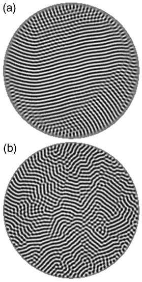
To study domain chaos we simulated Eq. (3) with fixed values of the nonlinear coefficients $g_{1}=1$, $g_{2}=-2.60$, and $g_{3}=1.5$ corresponding to a Kuppers-Lorz instability at an angle of $60{{}^{\circ}}$ CrossMeironTu94 . We studied the behavior for values of $\varepsilon$ between $0.01$ and $0.3$ and in circular geometries with radii $30\pi$, $40\pi$, $50\pi$, and $80\pi$, corresponding to aspect ratios of $30-80$ in the experimental system. Snapshots of the field $\psi(x,y)$ from two runs are shown in Fig. (1). Notice the dependence of the domain size on the control parameter $\varepsilon$, and the comparable values of domain and system sizes at the smaller value of $\varepsilon$.

Figure 2: Inverse measured correlation length $\xi_{M}^{-1}$ as a function of control parameter $\varepsilon$ for various aspect ratios $\Gamma$. The lines are fits of the form $\xi_{M}^{-1}=a(\varepsilon-\varepsilon_{0})^{1/2}$.

The quantitative diagnostics of the state are based on the Fourier transform $\tilde{\psi}(\mathbf{k)}$ using a Hanning window over an inscribed square, following the same approach as in the experiments Ning93pre2 . The intensity $S(\mathbf{k})=|\tilde{\psi}(\mathbf{k})|^{2}$ is found to be concentrated on a ring in Fourier space near $k=1$ corresponding to the stripe periodicity of $2\pi$. The intensity varies with the angle around this ring, corresponding to the varying representation of domains of different stripe orientations in the pattern. This angular distribution varies with time as the domains evolve, and can be used to define the switching rate $\omega_{a}$. The correlation length of the pattern is defined as the average width of the ring in Fourier space $\xi_{M}=[\left\langle k^{2}\right\rangle-\left\langle k\right\rangle^{2}]^{-1/2}$ with

$$\left\langle k^{n}\right\rangle=\left\langle\frac{\int k^{n}S(\mathbf{k})d^{2}k}{\int S(\mathbf{k})d^{2}k}\right\rangle_{t}$$ (5)

where $\left\langle\,\right\rangle_{t}$ denotes a time average.

Figure 3: Plot of the inverse correlation length $\xi_{M}^{-1}$ scaled with $\varepsilon^{1/2}$ against the inverse aspect ratio $\Gamma^{-1}$ scaled by $\varepsilon^{-1/2}$ showing the collapse of data for different $\varepsilon$ and $\Gamma$ onto a single curve. The solid line is a fit to the empirical form $y=\sqrt{a^{2}+b^{2}x^{2}}$ yielding $a=0.091$ and $b=2.8$. The dashed lines show the asymptotic limits of this fit.

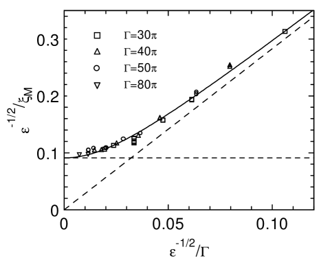
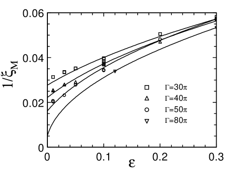
Results for the correlation length are shown in Fig. (2). As in the experiments the inverse of the measured correlation length $\xi_{M}^{-1}$ appears to remain nonzero at onset, and the data are reasonably well fit by a form $\xi_{M}^{-1}\sim\sqrt{\varepsilon-\varepsilon_{0}}$ rather than the expected $\sqrt{\varepsilon}$ dependence. The dependence of $\varepsilon_{0}$ we find on the aspect ratio suggests that this might be understood as a finite size effect. This is confirmed by the scaling plot motivated by Eq. (2) which suggests that a plot of $\varepsilon^{-1/2}/\xi_{M}$ against $\varepsilon^{-1/2}/\Gamma$ should collapse the data. The successful collapse is shown in Fig. (3). Note that for small values of $\varepsilon^{-1/2}/\Gamma$ (i.e. large $\Gamma$ or $\varepsilon$) the value of $\xi_{M}\varepsilon^{-1/2}$ approaches a constant corresponding to the theoretical expectation for large enough systems. On the other hand for large $\varepsilon^{-1/2}/\Gamma$ the curve approached a linear behavior consistent with the correlation length scaling simply with the aspect ratio, $\xi_{M}\simeq\Gamma/2.8$. Note that the finite size corrections become important (e.g. identified as the intersection point of the straight lines in Fig. (3) for $\Gamma\leq 3\xi$, with an additional factor of $3$ over the naive expectation.

In the experimental work there has been no systematic attempt to study the dependence on aspect ratio, which is much harder to do experimentally than numerically. The experiments did investigate the dependence of the correlation length on the rotation rate, and found that the measured correlation lengths at different rotation rates could be related by an $\varepsilon$-independent scale factor: $\xi(\varepsilon,\Omega)\simeq\xi_{0}(\Omega)f(\varepsilon)$. Since the deviation from the expected $\varepsilon^{-1/2}$ behavior found in $f(\varepsilon)$ is common to all the runs at different $\Omega$, this scaling does not shed light on the basic discrepancy with the predicted $\varepsilon^{-1/2}$ scaling however.

We have also studied the behavior of the switching frequency $\omega_{a}$ on $\varepsilon$. Here, unlike the experiment, we find good agreement with the prediction $\omega_{a}\propto\varepsilon$ for small $\varepsilon$ with no dependence on the aspect ratio. The trend $\omega_{a}\rightarrow 0$ for $\varepsilon\rightarrow 0$ even in finite size systems is not surprising for Eqs.(3,4) since the effects of the rotation that lead to the persistent dynamics only appear in the nonlinear terms which become small for $\varepsilon\rightarrow 0$. A careful analysis of the fluid equations shows that there are also linear terms depending on the rotation that are important near the boundaries. This means that in a finite system the onset of convection rolls in a rotating system is actually a Hopf bifurcation with the onset frequency going to zero for large aspect ratios, and so it might not be surprising that $\omega_{a}$ remains nonzero at onset. These effects can in fact be captured using modified boundary conditions for the Swift-Hohenberg equations Kuo94 . However these complicated boundary conditions make the numerical scheme considerably harder, and we have not modified our code to investigate them.

In conclusion our numerical simulations of model equations for rotating Rayleigh-Bénard convection show results for the correlation length near threshold that show qualitative similarities to the experimental results. A finite size scaling ansatz shows that our measured lengths are in fact consistent with the expected $\varepsilon^{-1/2}$ divergence near threshold, but that the finite system size obscures this dependence. It will be interesting to see if this result can be confirmed experimentally, or in simulations of the full fluid and heat equations for convection that we are currently pursuing. It is noteworthy that similar predictions for a diverging correlation time near threshold in electroconvection spatiotemporal chaos have recently been verified experimentally Toth98 . In this system larger aspect ratios are accessible so that finite size effects should not be important.