Classical 1D maps, quantum graphs and ensembles of unitary matrices

Abstract

We study a certain class of classical one dimensional piecewise linear maps. For these systems we introduce an infinite family of Markov partitions into equal cells. The symbolic dynamics generated by these systems is described by bistochastic (doubly stochastic) matrices. We analyze the structure of graphs generated from the corresponding symbolic dynamics. We demonstrate that the spectra of quantized graphs corresponding to the regular classical systems have locally Poissonian statistics, while quantized graphs derived from classically chaotic systems display statistical properties characteristic of Circular Unitary Ensemble, even though the corresponding unitary matrices are sparse.

I Introduction

Although graphs served as models of physical systems for a long time, the interest in properties of spectra of the corresponding quantum systems has rather short history. Quantum graphs were introduced as a “toy” model for studies of quantum chaos by Kottos and Smilansky [1, 2]. They observed that spectral statistics of fully connected graphs is well reproduced by random matrix theory (RMT) and may be explained using the exact trace formula. Schanz and Smilansky [3] proved that the spectral correlation function of simple graphs coincides with CUE expression for $2\times 2$ matrices. The trace formula served to calculate the spectral correlation function and to explain the deviations from the RMT predictions for star graphs [4]. Tanner introduced directed graphs and the corresponding unitary transfer matrices [5] and demonstrated fast convergence of their spectral properties to RMT statistics with increasing matrix size. A model for study of the Anderson localization by means of quantum graphs was introduced by Schanz and Smilansky [6], while other properties of quantum graphs were recently analyzed in [7, 8]. Continuous dynamics on graphs was recently discussed by Barra and Gaspard [9], who generated Markov process by means of Poincaré surface of section.

In this work we propose another approach leading to quantum graphs. We are interested in a certain class of one dimensional (1D) piecewise linear maps with infinite family of Markov partition into equal cells. For these systems we define a family of the corresponding graphs by means of bistochastic (doubly stochastic) transfer matrices $B$. If the transfer matrices are unistochastic (i.e. there exists a unitary matrix $U$ such that $B_{ij}=|U_{ij}|^{2}$) the graphs may be quantized. We may thus establish a family of the unitary transfer matrices by varying the lengths of bonds of graphs and investigate their spectra. We demonstrate a link between the character of dynamics of the classical system and the spectral properties of the corresponding ensemble of unitary matrices. For a class of regular 1D systems we show that the statistics of the spectrum is locally Poissonian. If the classical system has an arbitrary small, positive KS-entropy, the spectral statistics of the corresponding ensemble of unitary matrices displays fluctuations characteristic to Circular Unitary Ensemble (CUE) [10, 11]. These matrices are sparse (only few nonzero elements in each row and column) and by construction differ from typical random matrices generated according to the Haar measure on $U(N)$.

The paper is organized as follows. In section II we introduce the class of 1D maps of our interest. Section III contains an analysis of the structure and spectral properties of quantized graphs corresponding to regular systems. In section IV we study graphs corresponding to Bernoulli shift and to some systems with arbitrary small, but positive metric entropy. Section V is devoted to study of generic chaotic systems, for which we find CUE like spectral properties of the corresponding ensembles of unitary matrices. The concluding remarks are presented in section VI, while appendix A contains the condition necessary for a bistochastic matrix to be unistochastic and the calculation of free parameters for averaging over different graphs with the same topology. In appendix B we show the construction of unitary matrices corresponding to the classical map studied in section V.

II One dimensional dynamical systems

Consider a discrete one dimensional mapping acting on an interval $I\subset I\!\!R$

$$x_{n+1}=f(x_{n}),$$ (1)

where $f:I\rightarrow I$ is piecewise linear. Assume that $f$ fulfils three conditions:

1. there exists a Markov partition of the interval $I$ on $M$ equal cells $E_{i},i=1\dots M$ and $f$ is linear on each cell $E_{i}$,

2. for any $y\in I$

   $$\sum_{x\in f^{-1}(\{y\})}\frac{1}{f^{\prime}(x)}=1,$$ (2)

3. the finite transfer matrix $B$, describing the evolution of measures uniform on the cells of Markov partition, under the action of the system $f$ (the Frobenius-Perron operator) is unistochastic.

Condition (i) means that the graph of the function $f$ (later called diagram of $f$ to avoid the confusion with graphs corresponding to the map $f$) is composed of straight lines (neither horizontal nor vertical) with endpoints onto $M\times M$ grid on the square $I\times I$. Some examples of functions fulfilling this condition are plotted in figure 1. If we rescale $I$ to $[0,1]$ and write $f(x)=c_{j}x+b_{j}$ for $x\in I_{j}$ where $\bigcup_{j}I_{j}=I$, then all $c_{j}$ have to be nonzero integers and also, the numbers $b_{j}$ and $|I_{j}|/|I|$ must be rational (multiplication by a sufficiently large $M$ makes all these numbers integer). Any subpartition of the interval $I$ into $N=Mk$ equal cells ($k\in I\!\!N$) is also a Markov partition, so we have an infinite family of Markov partitions for our models. The Frobenius-Perron operator, reduced to densities (measures) constant on each cell $E_{j}$, may be described by a matrix $B$ of finite size $M$. Let us write the elements of $B$ explicitly. The system fulfilling the condition (i) is fully characterized by a set of $M$ linear functions

$$f_{i}(x)=c_{i}x+b_{i},\quad x\in\left[\frac{i-1}{M},\frac{i}{M}\right).$$ (3)

By construction $c_{i}$ and $Mb_{i}$ are both integers. It is convenient to express $c_{i}$ and $b_{i}$ in terms of two integers $l_{i}$ and $m_{i}$ as

$$c_{i}=m_{i}-l_{i},\quad b_{i}=\frac{m_{i}-i(m_{i}-l_{i})}{M}.$$ (4)

It is now easily seen that the only non-zero elements of $B$ in the $i$-th row are

$$B_{ij}=\frac{1}{|m_{i}-l_{i}|},\quad\min(m_{i},l_{i})+1\leq j\leq\max(m_{i},l_{i}).$$ (5)

Closer inspection of the structure of the above formula reveals the connection between the structure (positions of the non-zero elements) of the matrix $B$ and the diagram of the system $f$ rotated clockwise by $\pi/2$.

The element $B_{ij}$ is equal to the probability of going from the cell $E_{i}$ to $E_{j}$. From (5) $B$ is stochastic ($\sum_{j=1}^{N}B_{ij}=1$), all probabilities of going out of the cell $E_{i}$ sum to unity. The probability of coming to the cell $E_{j}$ from $E_{i}$ is equal to mean $1/|f^{\prime}(x)|$ over $x\in E_{i}$ and $f(x)\in E_{j}$. Thus due to condition (ii) the probabilities of transitions to any fixed cell $E_{j}$ also sum to one ($\sum_{i=1}^{N}B_{ij}=1$), so the transition matrix $B$ is bistochastic. It is well known that all eigenvalues of a bistochastic matrix are located in the unit circle, and the leading eigenvalue is equal to one [12]. The condition (iii) will be used in section V.

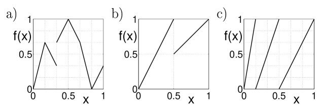
FIG. 1.: Examples of piecewise linear functions defining classical maps with Markov partition consisting of (a) $M=6$, (b) $M=2$ and (c) $M=6$ equal cells. Only system (a) fulfils (i)–(iii). Observe that the 1D system shown in panel (b) is regular even though the average slope exceeds unity, this system does not fulfil the condition (ii), the matrix $B$ corresponding to the system (c) is not unistochastic, so (iii) is violated.

We may compute the KS-entropy of Markov chain generated by transition matrix $B$ [13]

$$H_{KS}(B)=-\sum_{i=1}^{N}\tilde{p}_{i}\sum_{j=1}^{N}B_{ij}\log B_{ij},$$ (6)

where $\tilde{p}$ is the normalized left eigenvector of $B$ corresponding to the leading eigenvalue, $\tilde{p}B=\tilde{p}$, $\sum_{i=1}^{N}\tilde{p}_{i}=1$. In condition (i) we require that $f$ is linear (not only piecewise linear) on each cell $E_{j}$. Then the Markov partition on $M$ equal cells is a generating partition of the system, so Eq. (6) gives the dynamical entropy of the system. The transition matrix is bistochastic in our case, so all components of $\tilde{p}$ are nonzero ($\tilde{p}_{i}=1/N$) and $H_{KS}=0$ if and only if all $B_{ij}\in\{0,1\}$. It is easy to see that if $\forall x\in I:|f^{\prime}(x)|=1$ the system is regular. We have showed that this is also a necessary condition, provided the conditions (i) and (ii) are fulfilled, since only the systems with $|f^{\prime}|=1$ have all $B_{ij}\in\{0,1\}$. Note that in general there exist regular systems with slopes larger than one, but they do not satisfy the condition (ii). An example of such a system is plotted in Fig. 1(b).

III Regular systems

Partition of the interval $I$ determines the transition matrix $B_{ij}$ describing the symbolic dynamics of the 1D map $f(x)$. We introduce a directed graph with vertices corresponding to each cell $E_{i}$ of the partition and bonds corresponding to all nonzero elements of the transition matrix $B_{ij}$. Changing the number $N$ of the cells in the partition we change the dimension of the matrix $B^{(N)}$, so we may obtain a family of graphs corresponding to any 1D map fulfilling the condition (i).

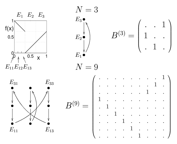
FIG. 2.: An example of a regular 1D system defined by function $f$ plotted in left top diagram, the corresponding graphs and the transition matrices representing Frobenius-Perron operators for Markov partitions into $N=3$ and $N=9$ cells. The dots represent zero elements of matrices. Note a link between the position of the nonzero elements of the matrices $B^{(N)}$ and the shape of the diagram of $f$ (rotated clockwise by $\pi/2$).

If we consider the regular systems with $|f^{\prime}|=1$ the only nonzero elements of matrices $B_{ij}$ are equal to 1. The matrices of this type contain only one nonzero element equal to 1 in each row and column and act as a permutation on a vector with $N$ elements. The corresponding graph has only one incoming and one outgoing bond at each vertex, so its valency is equal to one. It is composed from the closed loops. We say that there is an inversion at vertex $j$ of the graph if $f^{\prime}=-1$ on the corresponding cell $E_{j}$ of the partition. Dividing the interval $I$ into $M$ equal cells we find that the longest loop of the graph has at most $M$ vertices. If we consider a subpartition of $I$ into $N=Mk$ cells, each vertex of the graph will be replaced by $k$ vertices of a new graph. The loops with an even number of inversions will form $k$ new disconnected loops of the same period. The loops with an odd number of inversions will create $[k/2]$ disconnected loops with period doubled ($[\cdot]$ denotes the integer part of a number) and also, if $k$ is odd, one loop of the initial period. Fig. 2 shows an example of a regular system, for which the minimal Markov partition contains $M=3$ cells: $E_{1},E_{2},E_{3}$. Due to $f^{\prime}=-1$ in $E_{1}$ there exists one inversion in the 3-vertices graph corresponding to this system. For larger $N$ the graph is composed of $[k/2]$ loops with 6-vertices and one 3-vertices loop for an odd $k$. The classical map has one periodic orbit with period 3 and a continuous infinite family of orbits with period 6. Note similarity in the spectrum of periods of periodic orbits of the map and the graph for large odd $k$.

The quantization of a directed graph may be related to problem of finding a unitary matrix $U$, such as $|U_{ij}|^{2}=B_{ij}$ for all indices $i,j$ [5]. The matrix $U$ may be seen as a Floquet operator governing the discrete time evolution, while $U^{n}$ represents the evolution operator at discrete time $t=n$. Analyzing quantum maps, corresponding to time dependent periodical systems, one studies the statistical properties of phases of the unimodular eigenvalues of the unitary matrix $U$ [14]. The elements of $U$ may be expressed by $U_{ij}=r_{ij}e^{iL_{ij}}$, where the modulus are fixed by the transition matrix $r_{ij}=\sqrt{B_{ij}}$, and the phases $L_{ij}$, corresponding to lengths of the bonds of the graph, are not specified by the corresponding 1D map. We only impose that they fulfil the condition of unitarity $U^{\dagger}U={\mathbf{1}}$. Varying the phases $L_{ij}$ we obtain a family of graphs – an ensemble of unitary matrices. This corresponds to varying the lengths of all bonds of the graph with its topology preserved. We are interested in spectral properties of the ensemble of unitary matrices defined in this way. If $B$ is a permutation matrix, there is only one nonzero element in each row and each column of $U$, so all phases $L_{ij}$ appearing in matrix $U$ are uncorrelated.

The $N\times N$ unitary matrix $U$ corresponding to a regular 1D system is composed of $M$ square diagonal or antidiagonal blocks of size $k$. For the system presented in Fig. 2 the matrix $U$ has the form

$$U=\left(\begin{array}[]{ccc}0&0&V_{1}\\ V_{2}&0&0\\ 0&V_{3}&0\end{array}\right),$$ (7)

where $M=3$, $(V_{1})_{ml}=\delta_{m,k+1-l}e^{iL_{m}}$ is an antidiagonal $k\times k$ matrix, $(V_{2})_{ml}=\delta_{ml}e^{iL_{m+k}}$ and $(V_{3})_{ml}=\delta_{ml}e^{iL_{m+2k}}$ are diagonal matrices. There are $N$ free phases $L_{m}$ (the column index is superfluous here so we omit it). The eigenvalues of block matrix $U$ may be expressed by means of the spectra of its blocks $V_{i}$ [15]

$$\mbox{eig}(U)={}^{M}\sqrt{\mbox{eig}\left(V\right)}={}^{M}\sqrt{\mbox{eig}\left(\prod_{i=1}^{M}V_{i}\right)}\ ,$$ (8)

where the $M$-th root is a $M$ valued function. Unitary matrix $V=\prod_{i=1}^{M}V_{i}$ of size $k$ is diagonal or antidiagonal, depending on parity of the number of inversions in the corresponding loop in the basic $M$-vertex graph. The nonzero elements of $V$ are equal to $e^{i{\mathcal{L}}_{j}}$, where ${\mathcal{L}}_{j}$, $j=1\ldots k$ are sums of different phases $L_{m}$, so ${\mathcal{L}}_{j}$ are uncorrelated. If $V$ is diagonal the spectrum of $U$ consists of ${\{}e^{i({\mathcal{L}}_{j}+2\pi m)/M}{\}}^{j=1\ldots k}_{m=1\ldots M}$. The eigenphases of $U$ belonging to the same interval of the length $2\pi/M$ stem from different series ${\mathcal{L}}_{j}$, so they are uncorrelated and the spectrum has locally Poissonian statistics. If $V$ is antidiagonal, its spectrum contains $\sqrt{e^{i({\mathcal{L}}_{j}+{\mathcal{L}}_{k+1-j})}}$ and the spectrum of $U$ is composed of roots of unimodular complex numbers of order $2M$. The character of the spectrum remains Poissonian on the intervals of the length $\pi/M$.

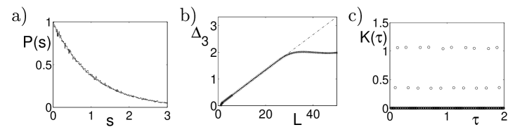
FIG. 3.: Spectral statistics for regular systems: (a) level spacing distribution $P(s)$, (b) spectral ridigity $\Delta_{3}(L)$ and (c) spectral form factor $K(\tau)$. The average is taken over an ensemble of $10^{5}$ matrices of the size $N=150$ with phases (bond lengths) chosen randomly. The statistics reveal deviations from the predictions of the Poissonian ensemble (dot dashed line) due to correlations on larger length scales.

The above argument may be generalized for the situation, in which the permutation matrix $B$ is reducible, composed of several permutations with different periods $M_{1}\ldots M_{p}$. In this case the eigenphases of $U$ are uncorrelated in intervals of length $\pi/\max M_{i}$. Fig. 3 shows the commonly used spectral statistics [11, 14] calculated for the system shown in Fig. 2. Note that the spectral ridigity $\Delta_{3}(L)$, which measures correlations in the spectrum at the length scale $L$, saturates at $L\approx 25=N/6$ (there are $N=150$ eigenphases rescaled to the mean density constant and equal to $1$). The divisor $6$ is equal twice the number of cells in minimal Markov partition, since an inversion in one of the cells occurs ($f^{\prime}(x)=-1$ for $x\in E_{1}$).

IV Simple chaotic systems

The Bernoulli shift, $f(x)=2x\ \mbox{mod}\ 1$, is one of the simplest 1D maps displaying chaotic dynamics. This system fulfils the conditions (i), (ii) and (iii). The graphs corresponding to this system were analyzed by Tanner [5]. The system, graphs and matrices are plotted in Fig. 4. Existence of a certain interval for which $|f^{\prime}(x)|>0$ causes the mean valency of the graphs to become larger than 1. Some vertices of the graphs have more than one outgoing bond, and this fact is related with a positive topological entropy of the corresponding classical map. The number of such vertices grows proportionally with $N$ and their presence is reflected in statistical properties of spectra of the corresponding unitary matrices. For the binary graphs all vertices have two outgoing bonds and as shown by Tanner [5] the spectral statistics converges fast to the predictions of CUE. The traces of the unitary evolution operator $U^{n}$ may be expressed by a sum over periodic orbits of the corresponding classical graph, analogous to the semiclassical Gutzwiller trace formula [16]. For quantum graphs the formula

$$\mbox{Tr}\ U^{n}=\sum_{\nu\in{\mathcal{PO}}(n)}A_{\nu}e^{iL_{\nu}}\ ,$$ (9)

is an identity, where ${\mathcal{PO}}(n)$ is the set of periodic orbits of period $n$, the amplitude $A_{\nu}=\prod_{(ij)\in\nu}\sqrt{B_{ij}}$ and the length $L_{\nu}$ is the sum of lengths of bonds belonging to the periodic orbit $\nu$.

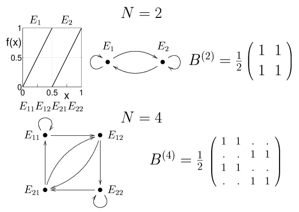
FIG. 4.: Bernoulli shift, the corresponding binary graphs and the matrices representing Frobenius-Perron operators for Markov partitions into $N=2$ and $N=4$ cells. Dots represent matrix elements equal to zero. For larger $N$ the structure of $B^{(N)}$ reflects the shape of $f(x)$.

We will show that every periodic orbit of the graph corresponds one to one to a periodic orbit of the dynamical system. Assume that $\nu=j_{1}j_{2}\ldots j_{n}$ is a periodic orbit of period $n$ of the graph, where $j_{i}$ denote the vertices belonging to $\nu$ and $|f^{\prime}|>1$ on at least one of the cells $E_{j_{c}}$. Let the functions

$$F_{j_{i}}:E_{j_{i+1}}\ni x\rightarrow f^{-1}(x)\in E_{j_{i}}$$ (10)

be the local inverse of $f$, where we identify $j_{1}$ and $j_{n+1}$. The function $F_{j_{c}}$ is a contracting mapping since $|F^{\prime}_{j_{c}}|\leq\frac{1}{2}$. We define

$$F=F_{j_{1}}\circ F_{j_{2}}\circ\ldots\circ F_{j_{n}}$$ (11)

which is a contraction of the cell $E_{j_{1}}$ onto itself, because $|F^{\prime}_{j_{i}}|\leq 1$ for $i\neq c$. The function $F$ corresponds to moving along the orbit backwards. Due to the Banach theorem there exists exactly one fixed point of $F$ in $E_{j_{1}}$, namely $x_{\nu}=F(x_{\nu})$. Hence there is a periodic orbit of period $n$ in the dynamical system corresponding to the orbit $\nu$ on the graph. The inverse is also true, so there is one to one correspondence between the orbits of the 1D chaotic system and the corresponding graphs.

The sum (9) goes over periodic orbits of the classical chaotic map. The amplitudes $A_{\nu}$, built from probabilities $B_{ij}$, are equal to $\prod_{i=0}^{n-1}1/|f^{\prime}(f^{i}(x_{\nu}))|^{1/2}$, so they are equal to the inverse square roots of the instabilities of the orbits of the system. Only the lengths $L_{\nu}$ are not determined yet, so we can average over the lengths of the bonds imposing the constraints due to unitarity of quantum propagator $U$. With growing dimension $N$ the spectral statistics of quantized binary graphs tends rapidly to the CUE statistics. Tanner observed it analyzing spectral form factors for graphs with rationally independent bond lengths [5]. Fig. 5 shows the spectral statistics averaged over an ensemble of $10^{5}$ matrices of $N=100$, corresponding to graphs with randomly chosen bond lengths (see appendix A).

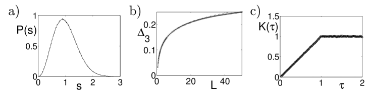
FIG. 5.: Spectral statistics for Tanner binary graphs averaged over bond lengths: (a) level spacing distribution $P(s)$, (b) spectral ridigity $\Delta_{3}(L)$ and (c) spectral form factor $K(\tau)$. The CUE prediction are represented by dot dashed lines (which almost coincide with the numerical data).

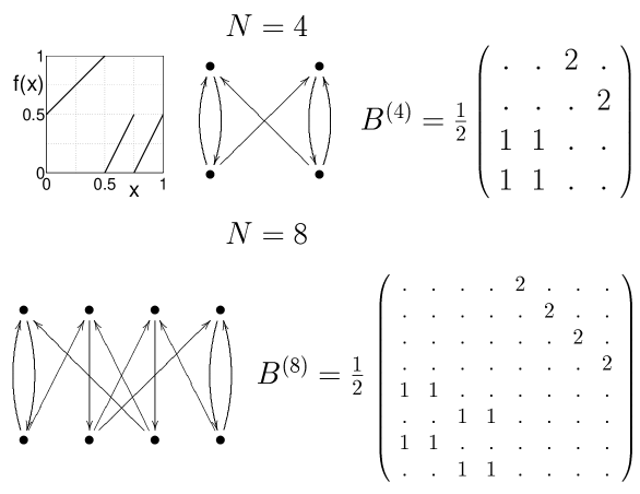
FIG. 6.: Chaotic system with $H_{KS}=\frac{1}{2}\ln 2$ and $\tilde{M}=2$, the function $f$ defining the system, the corresponding graphs and the transition matrices plotted for Markov partition into $N=4$ and $N=8$ cells. Zero elements of the matrices are marked by dots.

We may also analyze a system, for which $|f^{\prime}(x)|>1$ only in certain regions $I_{c}\subset I$. The KS-entropy of such a system is equal to the entropy of a system equivalent to $f(x)$ in $I_{c}$ times the ratio $\mbox{vol}(I_{c})/\mbox{vol}(I)$. This allows us to construct a system with an arbitrary small, positive KS-entropy. Consider the system presented in Fig. 6 with dynamical entropy $H_{KS}=\frac{1}{2}\ln 2$ (equal to the topological entropy), as an illustration of such situation. The structure of the unitary evolution operator $U$ is the same as the structure of the bistochastic transition matrix $B$ which is determined by the shape of the diagram of $f$. Block structure visible in Fig. 6 allows us to compute the spectra as in Eq. (8), where $V$ is the product of all blocks of $U$. If there is an even number of antidiagonal blocks, the resulting matrix $V$ is a product of one matrix with Poisson distribution of the spectrum and a certain number of non-diagonal matrices with a CUE-like spectrum. In ref. [17] we analyzed the spectra of composed ensembles consisting of products of random matrices, each pertaining to a given ensemble of unitary matrices. The CUE-like spectrum was found to be robust with respect to the multiplication by matrices of other ensembles. This is related to the fact that the Haar measure (CUE) is invariant with respect to multiplication. Following these lines of arguments, we conclude that the spectrum of $V$ has a CUE-like properties. The spectrum of $U$ is equal to the $\tilde{M}$-th root of the spectrum of $V$ ($\tilde{M}$ denotes the number of blocks in $U$)

$$e^{i\phi_{U}}=e^{i(\psi_{j}+2l\pi)/\tilde{M}}\ ,\qquad j=1\ldots k,\quad l=0\ldots\tilde{M}-1,$$ (12)

where $e^{i\psi_{j}}$ is the $j$-th eigenvalue of $V$, it consists of $\tilde{M}$ copies of the spectrum of $V$ contracted $\tilde{M}$ times and placed one after another, so its statistical properties are locally like these of CUE. Fig. 7 shows the statistical properties of an exemplary chaotic system presented in Fig. 6, for which all spectra consist of $\tilde{M}=2$ identical parts of length $\pi$. Note that the level spacing distribution and the spectral ridigity (for small $L$) show good agreement with the predictions of RMT. On the other hand the spectral form factor (i.e. the Fourier transform of the two point correlation function of the spectral density [14]) exhibits huge fluctuations since it measures correlations in the entire spectrum and reveals the presence of 2 copies of the same spectrum. However, the average taken over a small interval of $\tau=n/N$ displays a CUE-like behaviour.

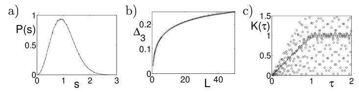
FIG. 7.: Spectral statistics for quantum graphs corresponding to the system shown in Fig. 6: (a) level spacing distribution $P(s)$, (b) spectral rigidity $\Delta_{3}(L)$ and (c) spectral form factor $K(\tau)$ averaged over $10^{5}$ matrices of size $N=200$. Dot dashed lines represent CUE statistics. The form factor displays large fluctuations, although the average over a window of $\tau$ of size $\Delta\tau=0.07$ (solid line) is close to CUE results.

Local agreement with the predictions of RMT is preserved even though there exist an inversion in the map $f$, which implies an antidiagonal blocks in $B^{(N)}$. To show this we analyzed a system consisting of 4 blocks, presented in Fig. 8, while the corresponding results are shown in Fig. 9.

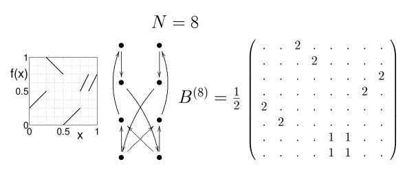
FIG. 8.: Chaotic system with $H_{KS}=\frac{1}{4}\ln 2$ and $\tilde{M}=4$, with an antidiagonal blocks in $B^{(N)}$: function $f$ defining the system, corresponding graph, and transition matrix. Find a link between its structure and the shape of $f(x)$.

In the argument presented in this section we have assumed that both parts of the system (one regular with $|f^{\prime}(x)|=1$ and the other chaotic with $|f^{\prime}(x)|>1$) are connected, so the probability of going from one to the other is positive. If this is not true, the system splits into two subsystems, one regular and one chaotic. The spectrum of such a system will contain a mixture of eigenvalues of both subsystems, so the level spacing statistics could be described by an appropriately adopted Berry-Robnik distribution [18].

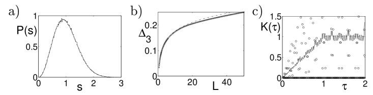
FIG. 9.: As in Fig. 7 for the system shown in Fig. 8.

V Generic systems

A generic 1D piecewise linear system fulfilling the conditions (i), (ii) and (iii) is chaotic and $|f^{\prime}(x)|\geq 2$ for all $x$ in $I$. The mean valency of the corresponding graphs is also equal to or greater than 2 and the topological entropy of these graphs $H_{\mbox{top}}$ is not smaller than $\ln 2$. The topological entropy of the map $f$ is equal to the log of the spectral radius (absolute value of the largest eigenvalue) of the connectivity matrix $\tilde{B}$ [13], where $\tilde{B}_{ij}=1$ if $B_{ij}>0$, and $\tilde{B}_{ij}=0$ otherwise. It is worth to consider, which of these graphs one may quantize by constructing corresponding family of unitary matrices. It is equivalent to ask, which bistochastic transition matrices $B$, are unistochastic, so there exist unitary $U$, such that $|U_{ij}|^{2}=B_{ij}$. It is clear that not all dynamical systems fulfilling (i) and (ii) give rise to bistochastic Frobenius-Perron matrices, which are unistochastic. As an example let us consider the system with $M=6$ shown in Fig. 1(c)

$$\begin{array}[]{lr}f_{1}(x)=6x,&\text{for }0\leq x<\frac{1}{6},\\ f_{2,3}(x)=3x-\frac{1}{2},&\text{for }\frac{1}{6}\leq x<\frac{1}{2},\\ f_{4,5,6}(x)=2x-1,&\text{for }\frac{1}{2}\leq x\leq 1.\end{array}$$ (13)

The corresponding transfer matrix

$$B=\frac{1}{6}\left[\begin{array}[]{cccccc}1&1&1&1&1&1\\ 2&2&2&0&0&0\\ 0&0&0&2&2&2\\ 3&3&0&0&0&0\\ 0&0&3&3&0&0\\ 0&0&0&0&3&3\end{array}\right]$$ (14)

is clearly bistochastic but not unistochastic. Indeed one checks that the necessary conditions for unistochasticity are not fulfilled (see Appendix A Eq. (A6), $k=3$ and $l=5$). This is the smallest matrix corresponding to a dynamical system of the considered type with this property, some other may be constructed for $M=28=14+7+4+2+1$ or other perfect numbers. In appendix A we present a necessary condition for unistochasticity and discuss some features of the ensemble of matrices $U$ corresponding to the same bistochastic matrix $B$.

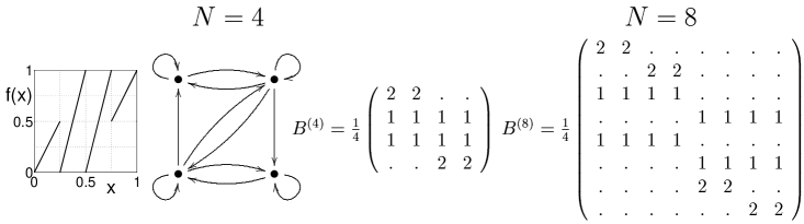
FIG. 10.: Classically chaotic 1D map (“four legs map”), corresponding graph and the transition matrices for Markov partitions into $N=4$ and $N=8$ cells. The slope of the map $f$ in each cell $E_{i}$ determines the size of elements in each row of the matrix $B^{(N)}$.

One of the maps studied by Dellnitz et al. [19] and showed in Fig. 10, may serve as an example of a classical map, for which transition matrices $B$ are unistochastic (see Appendix B). Its KS-entropy is equal to $\frac{3}{2}\ln 2$, while the topological entropy equals to $\ln 3$. Instead of computing the spectral radius of $\tilde{B}^{(4)}$ it is enough to observe that each point in $I$ has exactly three preimages, and the topological entropy may be computed as log of the mean number of preimages [20]. The average should be taken with respect to the Parry measure of maximal entropy [13], which is not easy to specify in the general case. However, since the number of preimages is constant, its knowledge is not necessary in this case to obtain the required result $H_{\mathrm{top}}=\ln 3$. Numerical investigations performed for the corresponding ensemble of $10^{5}$ matrices of size $N=200$ confirmed a CUE-like character of spectral statistics in the entire circle of eigenvalues as shown in Fig. 11.

FIG. 11.: As in Fig. 7 for the four legs map shown in Fig. 10.

Instead of averaging over an entire ensemble of unitary matrices with random phases, we may study spectral statistics for one concrete member of the ensemble. Figure 12 shows the spectral statistics for a single matrix $U$, in which the phases, not determined by unitarity, being set randomly (see Appendix A). Observe an agreement with CUE predictions (the form factor $K(\tau)$ is averaged over the window of $\tau$, $\Delta\tau=0.08$). Interestingly, for this system a CUE-like behaviour was also found for a single matrix $U_{0}$ (corresponding to the map plotted in Fig. 10) with all free parameters set to zero (thus exhibiting strong correlations between phases). Matrix $U_{0}$ is real (therefore orthogonal).

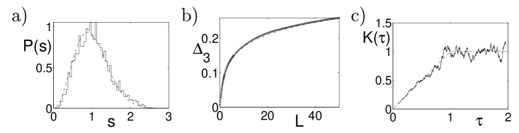
FIG. 12.: As in Fig. 7 for the four legs map shown in Fig. 10, without averaging over the ensemble of unitary matrices. The statistics calculated from single matrix of size 2500 with randomly chosen free phases are plotted.

Although a single member of the ensemble displays CUE-like spectrum, the averaging over free phases provides larger statistics. The form factor may be expressed as a double sum over periodic orbits

$$K(\tau)=\frac{1}{N}\left\langle|\mbox{Tr}\ U^{n}|^{2}\right\rangle=\frac{1}{N}\left\langle\sum_{\nu,\nu^{\prime}\in{\mathcal{PO}}(n)}A_{\nu}A_{\nu^{\prime}}e^{i(L_{\nu}-L_{\nu^{\prime}})}\right\rangle,$$ (15)

where $\tau=n/N$ and the averaging goes over all allowed realizations of the graph (all bond lengths $L_{ij}$, for which unitarity of $U$ is preserved). The difference of the lengths of orbits is equal to $L_{\nu}-L_{\nu^{\prime}}=\sum_{(ij)\in\nu}L_{ij}-\sum_{(lm)\in\nu^{\prime}}L_{lm}$. Inserting new variables $\tilde{L}_{ij}=L_{ij}-L_{i1}-L_{1j}+L_{11}$ we have

$$L_{\nu}-L_{\nu^{\prime}}=\sum_{(ij)\in\nu}(\tilde{L}_{ij}+L_{i1}+L_{1j}-L_{11})-\sum_{(lm)\in\nu^{\prime}}(\tilde{L}_{lm}+L_{l1}+L_{1m}-L_{11}),$$ (16)

where the lengths $\tilde{L}_{ij},\ i,j=2\ldots N$ are fixed by the condition assuring unitarity of $U$ (see Appendix A), while $(2N-1)$ remaining phases $L_{i1}$ and $L_{1j}$ are drawn randomly with a uniform distribution on $[0,2\pi)$. Due to averaging over $L_{i1}$, $L_{1j}$ the only non vanishing terms in the sum (15) arise from periodic orbits $\nu$ and $\nu^{\prime}$ of the same degeneracy class which visit each vertex of the graph the same number of times. This observation generalizes results of Tanner for binary graphs [5]. Therefore the calculation of $K(\tau)$ can be reduced to a combinatorial problem after finding the fixed lengths $\tilde{L}_{ij}$. The calculations of form factor for fully connected graphs [2] and binary graphs [5] shows fast convergence of the spectral statistics to RMT predictions with increasing matrix size $N$.

VI Conclusions

We proposed to study a certain class of piecewise linear 1D dynamical systems, for which the Markov transition matrix (of size $M$) is bistochastic. It has a structure of the diagram of $f$, defining the classical map, rotated clockwise by $\pi/2$. For each subpartition of the Markov partition we construct a graph and a family of unitary matrices, of size equal to a multiplicity of $M$. This procedure might be thus considered as a “quantization” of a $1D$ classical maps, in a sense that it produces a family of corresponding unitary matrices. The above quotation marks represent the fact that no canonical action-angle quantization of classical systems with 1D phase space is possible.

We demonstrated that the spectral properties of ensembles of unitary matrices defined in this way reflect the character of the classical dynamics. For regular maps the graphs are composed of several finite disconnected loops and the spectral statistics of the corresponding unitary evolution operators is (locally) Poissonian. On the other hand, chaotic systems (with arbitrarily small, but positive metric entropy), lead to ensembles of unitary matrices with (locally) CUE-like spectral fluctuations. These unitary matrices are sparse (only a few non zero elements in each row and column), in contrast to the random matrices, typical with respect to the Haar measure on $U(N)$.

We have shown that the classical 1D system and the corresponding family of graphs are topologically conjugated, since each periodic orbit of the map corresponds to exactly one periodic orbit of each graph. Applying finer and finer Markov partitions to the system, introduces a natural limit in the family of the corresponding graphs. It is the limit of number of vertices tending to infinity with the set of periodic orbits preserved. This seems to be the correct limit to reach random matrix theory predictions for the spectral statistics of quantized graphs. Spectral properties of a graph may be expressed by the exact trace formula based on a sum over periodic orbits. This sum goes over all periodic orbits of the 1D system and the amplitudes are equal to inverse square roots of the instabilities of each orbit. The phases in the sum remain free parameters of the model, with constraints due to unitarity of the evolution operator. We find conditions necessary for a bistochastic transfer matrix to be unistochastic, which allow us to perform averaging over random phases (bond lengths) with unitarity preserved.

Note added in proof

After this work was completed we learnt about very recent related works on unistochastic matrices of Berkolaiko [21] and Tanner [22].

A Unistochastic matrices

For a real bistochastic matrix $B$ of size $N$

$$B_{jk}\geq 0,\quad\sum_{j=1}^{N}B_{jk}=1,\quad\sum_{k=1}^{N}B_{jk}=1,$$ (A1)

we want to find a unitary matrix $U$, such that $|U_{jk}|^{2}=B_{jk}$. We can manipulate with $N^{2}$ variable phases $L_{jk}$ of the matrix $U$

$$U_{jk}=\sqrt{B_{jk}}\,\,e^{iL_{jk}}\ .$$ (A2)

The unitarity of $U$ requires that

$$U^{\dagger}U={\mathbf{1}}\quad\Leftrightarrow\quad\sum_{j=1}^{N}\sqrt{B_{kj}B_{lj}}\,\,e^{i(L_{lj}-L_{kj})}=\delta_{kl}\ .$$ (A3)

Equations (A3) for $k=l$ are fulfilled due to stochasticity of $B$, Eq. (A1). Equations (A3) for $k<l$ are complex conjugated of these for $k>l$. Transforming the system of equations (A3)

$$U(U^{\dagger}U-{\mathbf{1}})U^{\dagger}=UU^{\dagger}(UU^{\dagger}-{\mathbf{1}})=0\quad\Rightarrow\quad UU^{\dagger}-{\mathbf{1}}=0$$ (A4)

we found that $(N-1)$ equations of the system are depending on the other ones, because the diagonal equations of the righthand side are equivalent to conditions for bistochasticity of $B$ – the first sum in Eq. (A1). We subtracted the unity from $N$ since there is one common condition stemming from each of the sums in Eq. (A1), $\sum_{ij=1}^{N}B_{ij}=N$. The number of independent real equations in (A3) equals thus $(N-1)^{2}$.

We introduce new variables $\tilde{L}_{kj}=L_{kj}-L_{k1}-L_{1j}+L_{11}$, so the equations (A3) are equivalent to

$$\sum_{j=1}^{N}\sqrt{B_{kj}B_{lj}}\,\,e^{i(\tilde{L}_{lj}-\tilde{L}_{kj})}=\delta_{kl}\ .$$ (A5)

Since $\tilde{L}_{k1}=\tilde{L}_{1j}=0$, so the $(N-1)^{2}$ equations (A3) depend on $(N-1)^{2}$ real independent variables $\tilde{L}_{kj},\ k,j=2\ldots N$. These equations give the values of $\tilde{L}_{kj}$. For $N=2$ there exists only one phase $\tilde{L}_{22}$ equal to $\pi$ as shown by Tanner [5]. This value does not depend on the bistochastic matrix $B_{jk}$. Eqs. (A5) do not depend on $L_{k1}$ and $L_{1j}$, so we may average over them, assuming the uniform distribution over the unit circle, $P(L)=\frac{1}{2\pi}$ for $L\in[0,2\pi)$. This is equivalent to averaging of the matrix $U=D_{1}\tilde{U}D_{2}$ over diagonal unitary random matrices $D_{1}$ and $D_{2}$, with a fixed matrix $\tilde{U}$, fulfilling $|\tilde{U}_{jk}|^{2}=B_{jk}$.

The system of equations (A3) is solvable only if

$$\forall\,k\neq l\quad\max_{m=1\ldots N}\sqrt{B_{km}B_{lm}}\leq\frac{1}{2}\sum_{j=1}^{N}\sqrt{B_{kj}B_{lj}}\quad\mbox{and}\quad\max_{m=1\ldots N}\sqrt{B_{mk}B_{ml}}\leq\frac{1}{2}\sum_{j=1}^{N}\sqrt{B_{jk}B_{jl}}$$ (A6)

which is the condition for the possibility of balance the maximal term in the sums (A3) by the rest and the analog condition for the sums stemming from (A4). This necessary condition for a bistochastic matrix to be unistochastic becomes sufficient in $3\times 3$ case. For $N=2$ all bistochastic matrices are orthostochastic (and therefore also unistochastic). However for $N\geq 3$ several examples of bistochastic matrices, which are not unistochastic, are known [12], they do not satisfy the condition (A6). Statistical properties of random unistochastic matrices are studied in [23].

B Construction of a family of quantum maps

The construction of quantum graphs presented in section V hinge on the possibility of finding an unitary (or orthogonal) matrix corresponding to the bistochastic matrix obtained for a given dynamical system for an arbitrary Markov subdivision of the original partition. Rather then attempting the formulation of the most general theorem concerning the existence of such unistochastic matrices, we present here a construction for a particular case of the “four legs map” presented in Fig. 10. In other words we show that the all bistochastic matrices $B^{(N)}$ corresponding to this classical dynamical system are unistochastic.

The original bistochastic matrix for the “four legs map” introduced in [19] for the initial Markov partition into four cells reads

$$B^{(4)}=\frac{1}{4}\left(\begin{array}[]{cccc}2&2&0&0\\ 1&1&1&1\\ 1&1&1&1\\ 0&0&2&2\end{array}\right)\ .$$ (B1)

Let us consider the following choice of a corresponding unitary matrix

$$U^{(4)}=\frac{1}{2}\left(\begin{array}[]{cccc}\sqrt{2}&-\sqrt{2}&0&0\\ 1&1&1&1\\ 1&1&-1&-1\\ 0&0&\sqrt{2}&-\sqrt{2}\end{array}\right)\ .$$ (B2)

The bistochastic matrix for the two times finer subdivision reads

$$B^{(8)}=\frac{1}{4}\left(\begin{array}[]{cccccccc}2&2&0&0&0&0&0&0\\ 0&0&2&2&0&0&0&0\\ 1&1&1&1&0&0&0&0\\ 0&0&0&0&1&1&1&1\\ 1&1&1&1&0&0&0&0\\ 0&0&0&0&1&1&1&1\\ 0&0&0&0&2&2&0&0\\ 0&0&0&0&0&0&2&2\end{array}\right)\ .$$ (B3)

Using our knowledge of the unitarity of $U^{(4)}$ we want to find a unitary matrix $U^{(8)}$, such that $B^{(8)}_{ij}=|U^{(8)}_{ij}|^{2}$. This can be done by replicating twice the rows of $U^{(4)}$ with an appropriate shift. Thus $U^{(8)}$ may read as follows

$$U^{(8)}=\frac{1}{2}\left(\begin{array}[]{cccccccc}\sqrt{2}&-\sqrt{2}&0&0&0&0&0&0\\ 0&0&\sqrt{2}&-\sqrt{2}&0&0&0&0\\ 1&1&1&1&0&0&0&0\\ 0&0&0&0&1&1&1&1\\ 1&1&-1&-1&0&0&0&0\\ 0&0&0&0&1&1&-1&-1\\ 0&0&0&0&\sqrt{2}&-\sqrt{2}&0&0\\ 0&0&0&0&0&0&\sqrt{2}&-\sqrt{2}\end{array}\right)\ .$$ (B4)

Note that the number of the non zero elements in $U^{(8)}$ is two times larger than the number of the non zero elements in $U^{(4)}$. By replicating each row of the matrix $U^{(4)}$ $k$ times we obtain in the similar way unitary matrices of the size $4k$.

The success of this construction is due to the fact that the nonzero elements of the first and fourth rows of $U^{(4)}$ are equal, which implies orthogonality of the following pairs of rows in $U^{(8)}$: (2,3), (2,5), (4,7) and (6,7). However this is not the only way of constructing the family of unitary matrices $U^{(N)}$. For example we found another family $\tilde{U}^{(N)}$ originating from

$$\tilde{U}^{(4)}=\frac{1}{2}\left(\begin{array}[]{cccc}\sqrt{2}&-\sqrt{2}&0&0\\ 1&1&-1&1\\ 1&1&1&-1\\ 0&0&\sqrt{2}&\sqrt{2}\end{array}\right)\ ,$$ (B5)

even though the procedure described above fails in this case. This fact allows us to hope that the class of classical 1D maps leading to quantum graphs (fulfilling the conditions (i), (ii) and (iii)) is not trivial.

REFERENCES

- [1] Kottos T and Smilansky U 1997 Phys. Rev. Lett. 79 4794
- [2] Kottos T and Smilansky U 1999 Ann. Phys. NY 274 76
- [3] Schanz H and Smilansky U 1999 Proc. Australian Summer School in Quantum Chaos and Mesoscopics (Canberra), preprint Spectral Statistics for Quantum Graphs: Periodic Orbits and Combinatorics chao-dyn/9904007
- [4] Berkolaiko G and Keating J P 1999 J. Phys. A: Math. Gen. 32 7814
- [5] Tanner G 2000 J. Phys. A: Math. Gen. 33 3567
- [6] Schanz H and Smilansky U 2000 Phys. Rev. Lett. 84 1427
- [7] Kottos T and Smilansky U 2000 Phys. Rev. Lett. 85 968
- [8] Barra F and Gaspard P 2000 J. Stat. Phys. 101 283
- [9] Barra F and Gaspard P 2001 Phys. Rev. E 63 066215
- [10] Dyson F J 1962 J. Math. Phys. 3 140, 157, 166
- [11] Mehta M L 1991 Random Matrices 2 ed. (New York: Academic Press)
- [12] Marshall A W and Olkin I 1979 The Theory of Majorizations and Its Applications (New York: Academic Press)
- [13] Katok A and Hasselblatt B 1995 Introduction to the Modern Theory of Dynamical Systems (Cambridge: Cambridge University Press)
- [14] Haake F 1991 Quantum Signatures of Chaos (Berlin: Springer-Verlag)
- [15] Gantmacher F R 1959 The Theory of Matrices volumes 1 and 2 (New York: Chelsea)
- [16] Gutzwiller M C 1990 Chaos in Classical and Quantum Mechanics (Berlin: Springer-Verlag)
- [17] Poźniak M, Życzkowski K and Kuś M 1998 J. Phys. A: Math. Gen. 31 1059
- [18] Berry M V and Robnik M 1984 J. Phys. A: Math. Gen. 17 2413
- [19] Dellnitz M, Froyland G and Sertl S 2000 Nonlinearity 13 1171
- [20] Życzkowski K and Bollt E M 1999 Physica D 132 393
- [21] Berkolaiko G 2001 J. Phys. A: Math. Gen. 34 L319
- [22] Tanner G 2001 J. Phys. A: Math. Gen. 34 8485
- [23] Życzkowski K, Słomczyński W, Kuś M and Sommers H-J. to be published