Destabilization and Localization of Traveling Waves by an Advected Field

Abstract

We study a model of small-amplitude traveling waves arising in a supercritical Hopf-bifurcation, that are coupled to a slowly varying, real field. The field is advected by the waves and, in turn, affects their stability via a coupling to the growth rate. In the absence of dispersion we identify two distinct shortwave instabilities. One instability induces a phase slip of the waves and a corresponding reduction of the winding number, while the other leads to a modulated wave structure. The bifurcation to modulated waves can be either forward or backward, in the latter case permitting the existence of localized, traveling pulses which are bistable with the basic, conductive state.

1 Introduction

Various systems have been shown to exhibit bifurcations to spatially periodic patterns in the presence of an additional, weakly damped mode. If that mode corresponds to a conserved quantity it constitutes a true zero mode as in, e.g., translation of the fluid interface in two-layer Couette flow [1] or a shift in the displacement velocity of seismic waves in a viscoelastic medium [2]. Examples of weakly damped modes include the large-scale concentration field in binary-fluid convection [3, 4] or the real, slow mode in the 4-species Oregonator model of the BZ reaction [5]. The evolution of instabilities in these and similar systems will be coupled to the dynamics of the weakly-damped mode. Within the context of a weakly nonlinear approach near onset of the pattern-forming instability, the Ginzburg-Landau model is altered through the coupling to an evolution equation for the additional mode. The precise form of the coupling depends on the physics and symmetries of the system.

Steady instabilities in conserved systems with and without reflection symmetry have been considered. With reflection symmetry the instability, setting in at finite wavenumber, was found by Mathews and Cox [6] to be amplitude-driven, leading to a supercritical modulation of the underlying pattern. In the absence of reflection symmetry, Malomed [2] identified modulated patterns by deriving longwave equations for the phase of the underlying pattern coupled to the zero-mode. A particle-in-a-potential model in a moving frame was then derived for the local wavenumber, which admits both traveling and steady modulations. Ipsen and Sørensen [5] investigated the effect of a real, slow mode in reaction- diffusion systems near a supercritical Hopf bifurcation. They found the slow mode leads to new finite-wavenumber instabilities which alter traditional Eckhaus and Benjamin-Feir stability criteria for periodic waves. Barthelet and Charru [7] studied instabilities of interfacial waves in two-layer Couette-Poiseuille flow with Galilean invariance and no reflection symmetry, where the zero-mode is a shift of the fluid interface. The corresponding model of waves coupled to the zero-mode, derived and worked out by Renardy and Renardy [8], results in multiple, separated stability regions for periodic waves in contrast to the Eckhaus stable band exhibited by a single Ginzburg-Landau equation. The critically damped mode corresponding to a two-dimensional mean-flow in stress-free convection becomes relevant for not too large values of the Prandtl number. Bernoff [9] derived a Ginzburg-Landau equation coupled to the mean-flow mode from the Bousinesq equations and calculated the skew-varicose and oscillatory skew-varicose stability boundaries. This calculation brought into agreement previous work by both Siggia and Zippelius [10] and Busse and Bolton [11] who investigated the effect of mean-flow modes with non-zero vertical vorticity on the stability of rolls in Rayleigh-Benard convection.

In binary-fluid convection, Riecke [3] derived an amplitude equation for traveling waves arising in a Hopf bifurcation coupled to a critically damped mode related to large-scale modulations of the concentration field in the limit of small Lewis number. Instabilities of periodic waves within these equations were found to lead to localized traveling pulses which exhibited the anomalous slow drift observed in experiment [12], and in numerical simulations [13]. Riecke and Granzow presented a similar model on phenomenological grounds to describe the dynamics of traveling waves in electroconvection in nematic liquid crystals [14]. This model for oblique (zig and zag) waves coupled to a slow mode, possibly corresponding to a charge-carrier mode, exhibits instabilities to localized, worm-like structures as seen in experiment [15]. A striking feature of the worms is that although the extended waves bifurcate supercritically from the basic, conductive state, the worms themselves are bistable with the latter.

In the present paper, we consider traveling waves arising in a supercritical Hopf-bifurcation coupled to a real, slowly varying field. The field is advected by the waves and, in turn, can affect the dynamics of the waves through coupling to their growth rate. We briefly introduce the model and present a cursory linear analysis in section 2 which reveals distinct phase and amplitude instabilities of the waves. In sections 3 and 4 we are concerned with characterizing the linear and nonlinear behaviors of the phase and amplitude instabilities, respectively. In both cases we derive an envelope equation for the instability near its threshold and compare the results to full numerical simulations of the original equations. The envelope equations, in agreement with the numerics, indicate the phase-instability leads to a backward Hopf bifurcation, while the amplitude-driven instability leads to modulated waves, arising super- or subcritically. In the latter case, the subcritical branch can be bistable with the basic, conductive state and localized wave pulses arise.

2 The Extended Ginzburg-Landau Equations

We consider a model of a traveling wave with complex amplitude A and group velocity s coupled to a real, weakly damped mode C. The general form of the equations to orders $\epsilon^{3},\epsilon^{4}$ respectively, where $\epsilon$ is a measure of the distance from threshold of the bifurcation to traveling waves ($a_{1}=O(\epsilon^{2}$)), is dictated by symmetry,

$$\partial_{t}A+s\partial_{x}A = d_{1}\partial_{x}^{2}A+(a_{1}+a_{2}C)A-b|A|^{2}A,$$ (1)

$$\partial_{t}C = d_{2}\partial_{x}^{2}C-a_{3}C+a_{4}C^{2}+(h_{1}+h_{2}C)|A|^{2}+h_{3}|A|^{4}+h_{4}\partial_{x}|A|^{2}+h_{5}\partial_{x}^{2}|A|^{2}$$ (2)

$$+h_{6}i(\bar{A}\partial_{x}A-A\partial_{x}\bar{A})+h_{7}i\partial_{x}(\bar{A}\partial_{x}A-A\partial_{x}\bar{A})+h_{8}\partial_{x}A\partial_{x}\bar{A}.$$

The coefficients $d_{1},a_{1},a_{2},b$ in (1) are, in general, complex. The coefficients can be calculated for a particular system through a perturbative, normal-mode expansion of the relevant variables with slowly varying amplitudes,

$$\mathbf{\Phi}=\epsilon(\mathbf{u}A(x,t)e^{i(q\tilde{x}+\omega\tilde{t})}+c.c.)+\epsilon^{2}(\mathbf{v}C(x,t)+...)+h.o.t.$$ (3)

We consider a field $C$, that relaxes to a unique state in the absence of forcing by the wave and thus consider the contribution of the term proportional to $a_{4}$, which could introduce a second branch through a transcritical bifurcation, to be of higher order. We furthermore focus on the affect of advection by the traveling waves on C by retaining only the gradient coupling in (2) and eliminating the dispersion in (1). In the case of thermal binary fluid convection it turns out that the term proportional to $h_{1}$, which is formally of lower order than the gradient term, only contributes at higher order [16]. A gradient coupling of counterpropagating, traveling waves to a slowly varying field as a model for electroconvection in nematic liquid crystals has reproduced localized wave trains or ’worms’ seen in experiment [14]. In systems with a true zero mode (conserved quantity) certain terms like those involving $h_{1},h_{2},h_{3}$ and $h_{5}$ are not allowed and the gradient coupling is the relevant forcing [1], [6].

With the abovementioned simplifications, the system can be rewritten as,

$$\partial_{t}A+s\partial_{x}A = \partial_{x}^{2}A+(a+C)A-|A|^{2}A,$$ (4)

$$\partial_{t}C = \delta\partial_{x}^{2}C-\alpha C+h\partial_{x}|A|^{2}.$$ (5)

Equations (4, 5) describe the dynamics of a traveling wave without dispersion, which advects a real, slowly varying field C. The strength and sign of advection is given by the coefficient h. No homogeneous scaling is possible in these equations due to the presence of gradient terms which contribute to lower order in the limit of large-scale modulations. The scalings $\partial_{x}=O(\epsilon),\partial_{t}=O(\epsilon^{2})$ require $s=O(\epsilon),h=O(\epsilon)$ for strict validity of (4,5) indicating small group velocity and weak coupling. Modulations on a longer length scale ($\partial_{x}=O(\epsilon^{2})$) allow for O(1) values of s and h although the diffusive terms now contribute at higher order. The system thus becomes hyperbolic in this limit. Counterpropagating waves near onset have been studied in the hyperbolic limit [17], and can exhibit both sub- and supercritical secondary bifurcations as well as more complex dynamics. In this paper we choose not to reduce the equations (4,5) to a simpler form in a distinguished limit by fixing the scale. Instead we retain all terms as O(1) quantities and consider the equations as a phenomenological model of traveling waves coupled to a critically damped mode.

Our goal is to identify instabilities of waves in (4,5) and characterize their nonlinear evolution. We note that in the absence of coupling (h=0) or in the limit of rapid decay of the C-field ($\alpha\to\infty$) (4,5) reduce to a single Ginzburg-Landau equation which exhibits a long-wave phase instability for waves with wavenumber $q^{2}>\frac{a}{3}$. We shall refer to (4,5) as the extended Ginzburg-Landau equations (EGLE).

The complex amplitude A in (4) can be described by its real magnitude and phase $A=Re^{i\theta}$. Thus, in a frame moving with the waves (4,5) can be decomposed into the three following coupled equations,

$$\partial_{t}R = \partial_{x}^{2}R+R[(a+C)-R^{2}-(\partial_{x}\theta)^{2}],$$ (6)

$$R^{2}\partial_{t}\theta = \partial_{x}[R^{2}\partial_{x}\theta],$$ (7)

$$\partial_{t}C = \delta\partial_{x}^{2}C-\alpha C+s\partial_{x}C+2hR\partial_{x}R.$$ (8)

To determine instabilities of the traveling waves we linearize about the wave solution by considering an ansatz,

$$R = \sqrt{a-q^{2}}+\epsilon\tilde{R}e^{ipx+\sigma t},$$ (9)

$$\theta = qx+\epsilon\tilde{\theta}e^{ipx+\sigma t},$$ (10)

$$C = \epsilon\tilde{C}e^{ipx+\sigma t}.$$ (11)

We first consider instabilities in the longwave limit by expanding the growth rate $\sigma$ for small $p$. The three eigenvalues, corresponding to the real amplitude, phase and $C$-field respectively, are,

$$\sigma_{amp}(p) = -2R^{2}-2\frac{ihR^{2}}{(2R^{2}-\alpha)}p$$ (12)

$$-\frac{[4R^{6}\beta-2shR^{4}\alpha+(R^{2}+2q^{2})(2R^{2}-\alpha)^{3}]}{R^{2}(2R^{2}-\alpha)^{3}}p^{2}+O(p^{3}),$$

$$\sigma_{phase}(p) = -D_{E}p^{2}+2\frac{ihq^{2}}{\alpha R^{2}}p^{3}-2\frac{q^{2}[\beta+\frac{\alpha^{2}q^{2}}{R^{4}}]}{\alpha^{2}R^{2}}p^{4}+O(p^{5}),$$ (13)

$$\sigma_{field}(p) = -\alpha+\frac{i(2R^{2}(s+h)-s\alpha)}{(2R^{2}-\alpha)}p$$ (14)

$$-\frac{[-4R^{4}\beta+2shR^{2}\alpha+(2R^{2}-\alpha)^{3}\delta]}{(2R^{2}-\alpha)}p^{2}+O(p^{3}).$$

Here $R^{2}=\sqrt{a-q^{2}}$ is the amplitude of the plane wave and,

$$D_{E}=\frac{R^{2}-2q^{2}}{R^{2}}.$$ (15)

The parameter $\beta=h(s+h)$ is introduced for simplicity; it will prove to be useful in characterizing the type of instability.

We notice that to leading order, the eigenvalues corresponding to the amplitude (12) and advected field (14) are negative for finite values of $R^{2}$ and $\alpha$. The critical mode, corresponding to the phase, exhibits a longwave instability when the diffusion coefficient $D_{E}$ changes sign; this occurs at the Eckhaus curve $q^{2}=\frac{a}{3}$. However, the coupling of the advected field now raises the possibility of the quartic order term balancing the quadratic term in (12) as $D_{E}\to 0$. This would indicate a small-, yet finite-wavenumber instability. Indeed, a necessary condition for this phase instability to occur is that $\beta+\frac{\alpha^{2}q^{2}}{R^{4}}<0$. Figure 1(a) shows the eigenvalue of the phase mode which exhibits this finite- wavenumber instability, i.e. sufficiently small wavenumbers are damped. In Figure 1(c) we see the corresponding linear stability diagram. Here plane waves become linearly unstable already before the Eckhaus curved is reached. However, we note that near onset of the traveling waves, i.e. as $a\to 0$ for finite $\alpha$, (4, 5) can be rescaled, and $C$ adiabatically eliminated to yield a single Ginzburg-Landau equation. In this limit the contribution of the C-field is formally of higher order and we recover the Eckhaus instability (cf. Fig. 2(a), below).

     

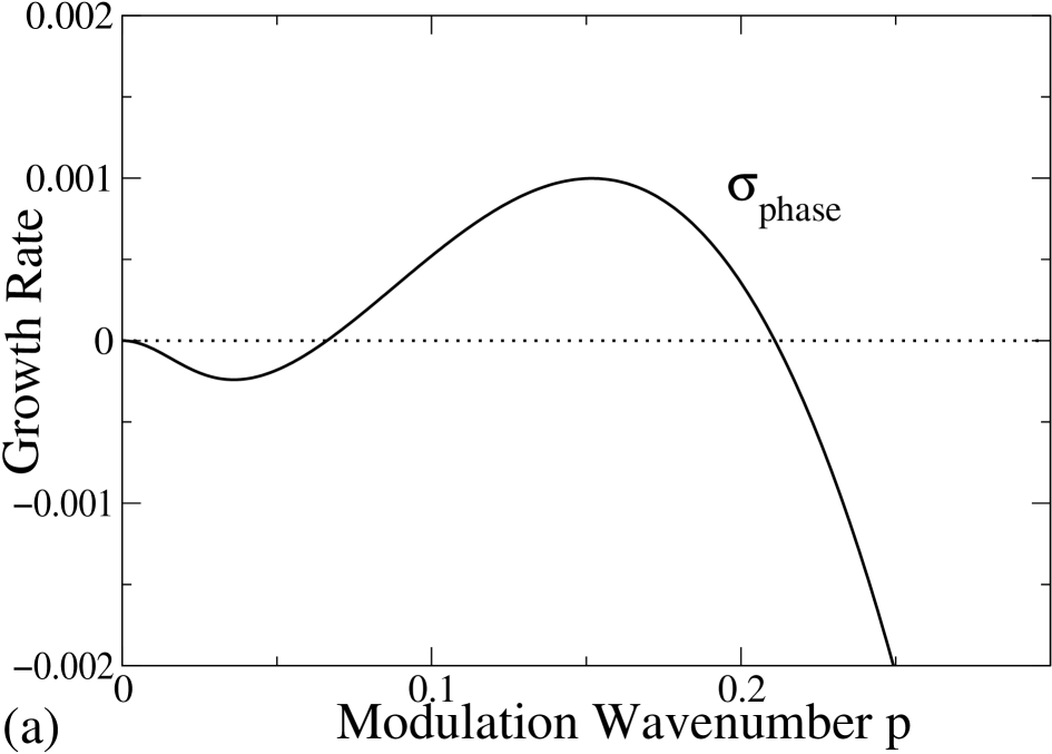
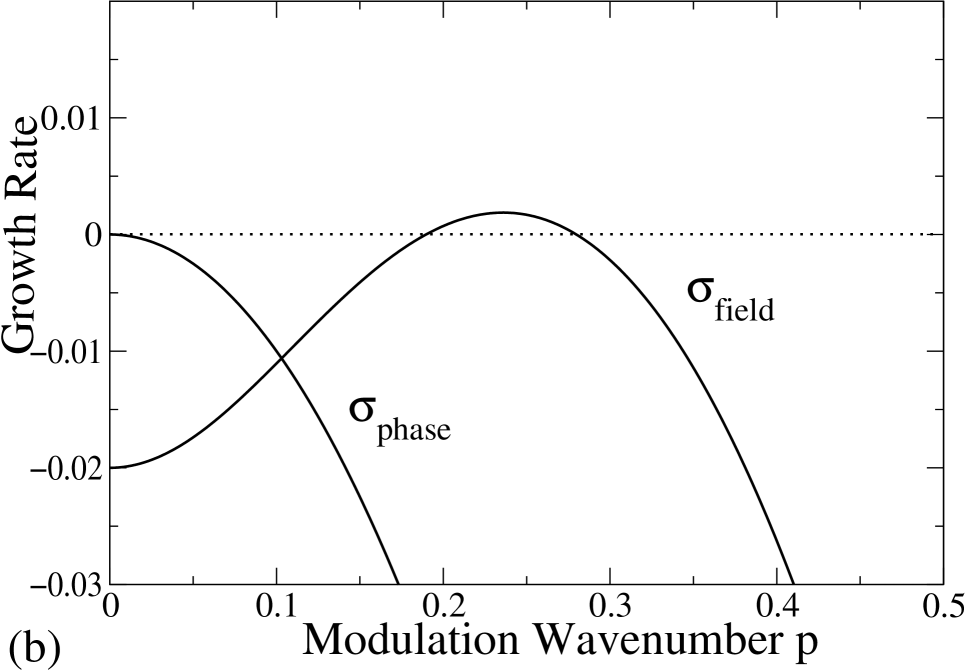
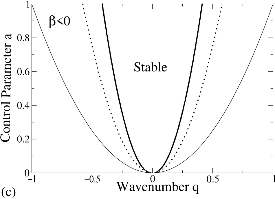
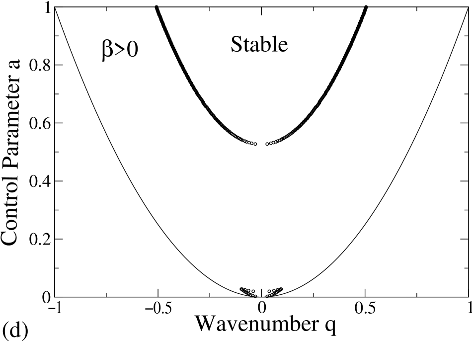
Figure 1: For all 4 figures h=1, $\alpha$=0.02, $\delta$=1.0 In (a) s=-1.5, q=0.425, a=1.0. This is a shortwave phase instability. The other two eigenvalues are large and negative. In (b) s=1.0, q=0, a=0.5. This is a shortwave instability of the C-field. The phase-eigenvalue is marginal for p=0 due to translation symmetry while the amplitude-eigenvalue is large and negative. (c) is the linear stability diagram for the values of the coefficients given in (a). The dotted line is the Eckhaus curve, given here for comparison. (d) is the linear stability diagram for the same coefficients as in (b).

Next consider waves which are phase-stable in this regime ($D_{E}>O(p^{2})$ or $\beta+\frac{\alpha^{2}q^{2}}{R^{4}}>0$ or both). In the limit as $\alpha\to 0$, the eigenvalue corresponding to the C-field can become positive through a balance between the leading order term and that at $O(p^{2})$. Consider, for example, the eigenvalues at bandcenter (q=0),

$$\sigma_{amp}(p) = -2a-2\frac{iha}{(2a-\alpha)}p-\frac{[4a^{2}\beta-2sha\alpha+(2a-\alpha)^{3}]}{(2a-\alpha)^{3}}p^{2}+O(p^{3}),$$ (16)

$$\sigma_{phase}(p) = -p^{2},$$ (17)

$$\sigma_{field}(p) = -\alpha+\frac{i(2a(s+h)-s\alpha)}{(2a-\alpha)}p-\frac{[-4a^{2}\beta+2sha\alpha+(2a-\alpha)^{3}\delta]}{(2a-\alpha)}p^{2}+O(p^{3}).$$ (18)

While for finite a as $\alpha\to 0$, both the amplitude and phase eigenvalues are stable the field-eigenvalue can become unstable if $-4\beta+8a\delta<0$. This condition can only be satisfied for $\beta>0$ and implies additionally that there is an upper bound on the control parameter a for fixed $\beta$ and $\delta$ above which this instability cannot exist ($a_{bound}=\frac{\beta}{2\delta}$). Such a case is seen in Figure 1(b) where the eigenvalue corresponding to modulations of the C-field indicates positive growth for finite-wavenumber perturbations. The linear stability diagram Figure 1(d) confirms the existence of the linear instability over a finite range of the control parameter $a$, resulting in a small stability-island near onset.

As $\beta$ passes from negative values through zero, the linear stability diagram given in Figure 1(c) changes continuously to that shown in 1(d). The intermediate regime is not captured analytically in the longwave expansions we have used thus far and must be investigated numerically. Figure 2(b) shows how the region of linear stability of the traveling waves changes as $\beta$ passes through zero. The stability boundary, outside of which the waves are phase-unstable to finite-wavenumber modulations for $\beta<0$, develops a bottle-necked region which pinches off as $\beta$ becomes more positive, resulting in two separated plane-wave-stable regions (cf. Fig.1(d)). This change is continuous, and there are values of $\beta$ for which numerical simulations have revealed both phase- and amplitude-instabilities. That is, amplitude-modulated waves can arise whose underlying phase undergoes slips until a phase-stable wavenumber is achieved.

     

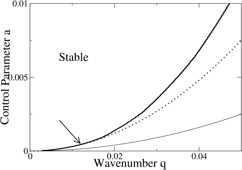
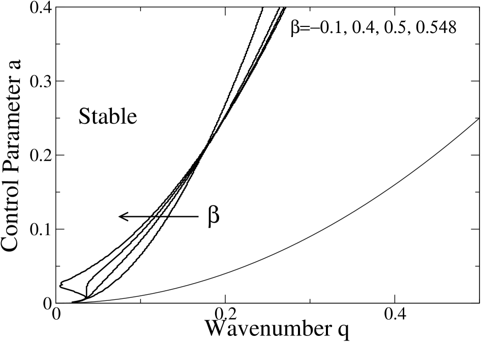
Figure 2: (a) Linear Stability diagram near threshold of the traveling waves ($a\ll 1$). The stability boundary approaches the Eckhaus curve as $a\to 0$ (arrow). (b) Linear stability diagram with $h$=1.0, $\alpha$=0.02, $\delta$=1.0, $s$=-1.1, -0.6, -0.5, -0.452. In this intermediate regime both phase and amplitude instabilities can set in.

3 Phase Instability

To facilitate the analysis of the phase instability, we make use of the large, negative eigenvalue of the magnitude of A to derive coupled phase and field equations in a longwave limit. If the longwave limit is taken at finite $\alpha$ both the magnitude and the advected field can be adiabatically eliminated and, to leading order, one obtains the usual phase equation with the usual Eckhaus stability limit. The effect of the $C$-field can be captured, however, in a distinguished longwave limit in which $\alpha\to 0$ as well. Then the amplitude can be adiabatically slaved to the dynamics of the phase and $C$-field, given that we are sufficiently far from the neutral stability boundary ($R^{2}\not\ll 1$).

We consider an ansatz of the form $A=R(T,X)e^{\frac{i}{\epsilon}\phi(T,X)}$, where $X=\epsilon x,T=\epsilon^{2}t$, and additionally $\alpha=\epsilon^{2}\alpha_{2}$. This scaling allows for large variations in the phase, although slow in time and space. To leading order we obtain an algebraic relationship relating the slaved amplitude to the C-field and local wavenumber,

$$R^{2}=a+C-(\partial_{X}\phi)^{2}.$$ (19)

Combining equations at orders $\epsilon$ and $\epsilon^{2}$ yields the longwave equations for the phase and the C-field,

$$\partial_{T}\phi = D_{E}\partial_{X}^{2}\phi+\frac{\partial_{X}\phi\partial_{X}C}{R^{2}},$$ (20)

$$\partial_{T}C = \delta\partial_{X}^{2}C-\alpha_{2}C+(s+h)\partial_{X}C-h\partial_{X}(\partial_{X}\phi)^{2}.$$ (21)

The phase-diffusion coefficient $D_{E}$ is defined as before (cf. (15)) where $R^{2}$ is now given by (19) and the local wavenumber is now given by the gradient of the phase, $q=\partial_{X}\phi$. As before, we linearize the longwave equations about the plane wave state with an ansatz,

$$\phi = qX+\epsilon\tilde{\phi}e^{ipX+\sigma T},$$ (22)

$$C = \epsilon\tilde{C}e^{ipX+\sigma T}.$$ (23)

The linearized longwave equations yield a complex, quadratic dispersion relation. As for the full EGLE we expand the growth rate $\sigma$ in powers of the modulation wavenumber $p$,

$$\sigma_{phase}(p) = -D_{E}p^{2}+2\frac{ihq^{2}}{R^{2}\alpha_{2}}p^{3}-2\frac{q^{2}\beta}{R^{2}\alpha_{2}^{2}}p^{4}+O(p^{5}),$$ (24)

$$\sigma_{field}(p) = -\alpha_{2}+i(s+h)p-\delta p^{2}+O(p^{3}).$$ (25)

As expected, phase modes with infinitesimal wavenumber become unstable when $D_{E}$ changes sign. However, according to (24) for $\beta<0$ phase modes with finite wavenumber p become unstable already for $D_{E}>0$ if

$$p^{2}>2D_{E}\frac{R^{2}\alpha_{2}^{2}}{q^{2}\beta}.$$ (26)

Thus, although we have identified the instability in the longwave limit, it is a shortwave instability and to determine the value of the critical modulation wavenumber p for which $\sigma$ first passes through zero we must solve the dispersion relation exactly.

The action of the linearized operator of the longwave equations on (22, 23) yields a 2x2 matrix, the determinant of which must equal zero for a nontrivial solution to exist. If we consider the real and imaginary parts of the growth rate $\sigma=\sigma_{r}+i\omega$, this dispersion relation can be written as,

$$\sigma_{r}^{2}+c_{1}\sigma_{r}+c_{2} = 0,$$ (27)

$$c_{3}\sigma_{r}+c_{4} = 0,$$ (28)

where

$$c_{1} = (p_{1}^{2}(D_{E}+\delta)+\alpha_{2}),$$ (29)

$$c_{2} = -\omega^{2}+\omega p(s+h)+p_{1}^{2}D_{E}(p_{1}^{2}\delta+\alpha_{2}),$$ (30)

$$c_{3} = 2\omega-p(s+h),$$ (31)

$$c_{4} = \omega(p^{2}(D_{E}+\delta)+\alpha_{2})-\frac{p^{3}}{h}(D_{E}(\beta-h^{2})+h^{2}).$$ (32)

At criticality ($\sigma_{r}=0$), (28) and (32) yield the Hopf-frequency,

$$\omega_{Hopf}=\frac{p^{3}}{h}\frac{(D_{E}(\beta-h^{2})+h^{2})}{(p^{2}(D_{E}+\delta)+\alpha_{2})}.$$ (33)

From equations (27) and (30) we arrive at a bi-cubic polynomial in p, the roots of which give the critical modulation wavenumber for the oscillatory instability,

$$-p^{4}(D_{E}(\beta-h^{2})+h^{2})^{2}+p^{2}\beta(D_{E}(\beta-h^{2})+h^{2})(p^{2}(D_{E}+\delta)+\alpha_{2})+$$

$$h^{2}D_{E}(\delta p^{2}+\alpha_{2})(p^{2}(D_{E}+\delta)+\alpha_{2})^{2}=0.$$ (34)

Solving for p directly in the sixth-order polynomial is not analytically feasible, but we note that the parameter $\beta$ is merely quadratic in (31) and so seek a solution for $\beta$,

$$\beta_{1,2} = -\frac{h^{2}(1-D_{E})(p^{2}(\delta-D_{E})+\alpha_{2})}{2D_{E}(p^{2}\delta+\alpha_{2})}$$ (35)

$$\pm\frac{p(p^{2}(D_{E}+\delta)+\alpha_{2})}{2D_{E}p^{2}(p^{2}\delta+\alpha_{2})}\sqrt{h^{2}p^{2}(1-D_{E})^{2}-4D_{E}^{2}(p^{2}\delta+\alpha_{2})^{2}}.$$

It can be shown that $\sigma_{r}>0$ only if the real quantity $\beta=h(s+h)$ is in the range $\beta_{1}<\beta<\beta_{2}$. Thus, the finite-wavenumber instability can only arise if $\beta_{1,2}$ are real, requiring the discriminant to be positive, $h^{2}p^{2}(1-D_{E})^{2}>4D_{E}^{2}(p^{2}\delta+\alpha_{2})^{2}$. This can be interpreted as a constraint on the modulation wavenumber p,

$$|p^{2}-\frac{h^{2}(1-D_{E})^{2}-8D_{E}^{2}\delta\alpha_{2}}{8D_{E}^{2}\delta^{2}}|<\frac{h(1-D_{E})}{8D_{E}^{2}\delta^{2}}\sqrt{h^{2}(1-D_{E})^{2}-16D_{E}^{2}\delta\alpha_{2}}.$$ (36)

This implies the additional constraint $h^{2}(1-D_{E})^{2}>16D_{E}^{2}\delta\alpha_{2}$ which can be simplified to,

$$q^{2}>\frac{a}{3+\frac{|h|}{2\sqrt{\alpha_{2}\delta}}}.$$ (37)

This somewhat intricate analysis of (34) can now be summarized concisely. A sufficient condition for stability of the waves with respect to shortwave instabilities is that the underlying wavenumber of the waves be in the band given by $q^{2}<\frac{a}{3+\frac{|h|}{2\sqrt{\alpha_{2}\delta}}}$, which is narrowed with respect to the traditional Eckhaus band. Thus, with respect to phase instabilities, the band of stable wavenumbers is bounded below by (37) and above by the Eckhaus curve,

$$\frac{a}{3+\frac{|h|}{2\sqrt{\alpha_{2}\delta}}}<q_{phase}^{2}<\frac{a}{3}.$$ (38)

If (38) is satisfied there exists a range in $\beta$ given by (35) for which the plane wave is unstable. For a given $\beta$ from this range the destabilizing modulation wavenumbers are given by the condition that the associated interval $[\beta_{1},\beta_{2}]$ include that value of $\beta$.

     

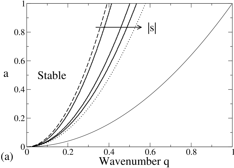
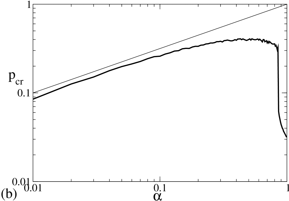
Figure 3: (a) Stability boundary as a function of the group velocity s. The boundary is bounded to the left by the stability condition derived from the dispersion relation of the longwave equations and to the right by the Eckhaus curve. Here h = 1, $\alpha$ = 0.02 $\delta$ = 1.0 and s = -1.5, -3.0, -5.0. (b) Dependence of the critical modulation wavenumber on the decay rate of C, $\alpha$. The thick line is numerically calculated from the full dispersion relation while the thinner line is p=$\sqrt{\frac{\alpha}{\delta}}$. (40) is thus valid only for small enough $\alpha$. ($a$=1.0, $h$=1.0, $s$=-1.5, $\delta$=1.0)

In the limit of zero coupling ($h\to 0$) or large decay rate of the concentration field ($\alpha_{2}\to\infty$) the Eckhaus band is recovered in a consistent manner. A linear stability diagram of waves as obtained from the full EGLE (1, 2) is shown in Figure 3(a) for various values of the group velocity s. It can be seen that inequality (38) is satisfied.

3.1 Weakly Nonlinear Analysis of Phase Instability

To examine the weakly-nonlinear behavior of the phase-instability one must solve (34) for given values of the system parameters. In the general case this yields a numerical value for the critical modulation wavenumber $p$ which can then be used in a weakly-nonlinear analysis. The coefficients of the resulting amplitude equation must then be evaluated numerically. However, if we restrict the wavenumber of the waves to lie on the curve representing the lower bound of existence of the shortwave instability, we can obtain analytical values for the critical modulation wavenumber and Hopf-frequency and consequently also for the coefficients of the amplitude equation. Along that curve,

$$q_{cr}^{2} = \frac{a_{0}}{3+\frac{|h|}{2\sqrt{\alpha_{2}\delta}}},$$ (39)

$$p_{cr}^{2} = \frac{\alpha_{2}}{\delta},$$ (40)

$$\omega_{cr} = -\textrm{sgn}(p_{cr}h)\frac{p_{cr}^{2}}{1+\frac{4\sqrt{\alpha_{2}\delta}}{|h|}},$$ (41)

$$\beta_{cr} = -4p_{cr}\delta\left(1-\frac{1}{2\delta(1+\frac{4\sqrt{\alpha\delta}}{|h|})}\right).$$ (42)

It is good to keep in mind that these values fix a unique value of the parameter $\beta=h(s+h)$ given by (42) and are in this sense restrictive. In addition, (39-41) are obtained in a longwave analysis, which requires that $p,\alpha\ll 1$. Figure 3(b) indicates the values of $\alpha$ for which (39-41) are valid.

We expand the phase and $C$-field in small-amplitude, normal modes, where $\epsilon=\sqrt{\frac{(a-a_{0})}{a_{2}}}$ is a measure of the distance from the bifurcation point ($a_{0},q_{cr}$),

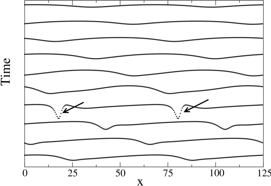
Figure 4: Space-time diagram of the evolution of the magnitude $|A|$ leading to a phase slip (arrows), here indicated by the dip in amplitude. s=-1.5, h=1 , $\alpha$ =0.02, $\delta$ =1.0

$$\left(\begin{array}[]{cc}\phi\\ C\end{array}\right)=\left(\begin{array}[]{cc}q_{cr}X\\ 0\end{array}\right)+\epsilon\Bigg{[}\left(\begin{array}[]{cc}\Phi_{0}\\ C_{0}\end{array}\right)A_{0}(\tau)e^{i(p_{cr}X+\omega_{cr}T)}+c.c+h.o.t.\Bigg{]}.$$ (43)

The complex amplitude $A_{0}$ of the unstable mode evolves on the superslow time scale $\tau=\epsilon^{2}T$. Inserting this ansatz into (20, 21) and solving order by order leads to a solvability condition at O($\epsilon^{3}$) which yields a differential equation for $A_{0}$,

$$\partial_{\tau}A_{0}=-\Sigma(a_{0},\alpha_{2},\delta,h)a_{2}A_{0}+\Gamma(a_{0},\alpha_{2},\delta,h)|A_{0}|^{2}A_{0}.$$ (44)

We are interested in the real part of the cubic coefficient, the sign of which gives the nature of the Hopf-bifurcation (forward/backward). The coefficient $\Gamma$ is a complicated expression of $\delta$, $\alpha_{2}$, a, and h, but we can expand it for small $\alpha_{2}$ to obtain an asymptotic approximation ($\alpha$ must be small from Figure 3(b)),

$$\Sigma = \frac{1}{(2\delta+1)}\Bigg{(}\frac{2|h|}{a_{0}^{3}\delta^{1/2}}\Bigg{)}^{1/2}(1+i\textrm{sgn}(h))\alpha_{2}^{3/4}+O(\alpha^{5/4}),$$ (45)

$$\Gamma = \frac{1}{a^{2}\delta^{3/2}(2\delta+1)}\Bigg{(}\frac{404}{5|h|}\alpha_{2}^{1/2}+i\textrm{sgn}(h)\Bigg{[}\frac{12}{\delta^{1/2}}+\frac{4}{5}\frac{(494\delta+451)}{(2\delta+1)}\alpha_{2}^{1/2}\Bigg{]}\Bigg{)}\alpha_{2}^{3}+O(\alpha_{2}^{9/4}).$$ (46)

Thus in the limit $\alpha_{2}\to 0$, $\Gamma>0$ for all values of the coefficients, and the phase mode undergoes a backward Hopf-bifurcation. Solving the coefficient $\Gamma$ numerically over a wide range of parameter values always yielded a positive real part. This analysis does not indicate whether or not the instability saturates at higher order or if the phase becomes undefined, signaling a phase slip. To investigate the nonlinear behavior of the phase, (1, 2) were integrated numerically using a linearized Crank-Nicholson scheme. It was found for the parameter values tested, that the waves outside the stability band underwent a phase slip when perturbed, relaxing to the plane-wave- stable band as seen in Figure 4, which shows a space-time diagram of the magnitude $|A|$ of the waves.

4 Amplitude Instability: Modulated Waves

We now investigate the instability corresponding to the eigenvalue of the $C$-field passing through zero in (18) which occurs only for $\beta>0$. Figure 5(a) indicates that plane waves are stable at onset, becoming linearly unstable as the control parameter is increased until , for large enough values of the control parameter, they once again regain stability. In addition, the band of stable wavenumbers is bounded by the Eckhaus curve outside the range of the amplitude instability. Thus for $\beta>0$ two distinct instabilities are possible depending on the wavenumber of the waves and the distance from threshold. Figure 5(b) shows the relevant eigenvalue as a function of the modulation wavenumber for increasing values of the control parameter. The wavenumber of the fastest growing mode increases continuously over the range of values of the control parameter for which the waves are linearly unstable.

     

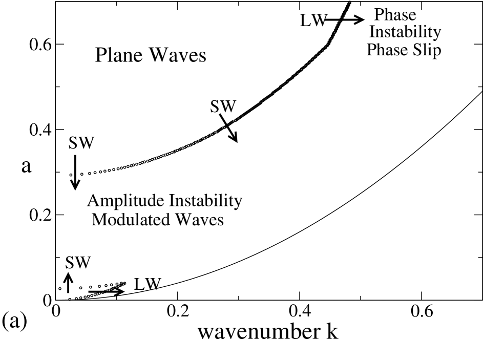
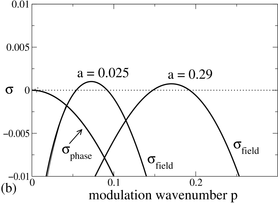
Figure 5: A linear stability diagram is given in (a) for h=1, s=1, $\alpha$=0.02, $\delta$=1.5. LW and SW denote longwave and shortwave instabilities respectively. In (b) the largest positive eigenvalue of the system is plotted versus the modulation wavenumber at bandcenter. Shortwave instabilities occur as the control parameter a is increased from the stable region near onset of the plane waves and as a is decreased from the stable region far beyond threshold.

At bandcenter, the system (6, 7, 8) decouples in the case of unperturbed plane waves. Perturbing the plane-wave solution with the ansatz (9, 10, 11) where q=0, introduces an order $\epsilon^{2}$ coupling of the phase to the real amplitude through $(\partial_{x}\theta)^{2}$, which does not appear in the linearized system. Thus it is sufficient to consider the following equations for the linear stability of the waves at bandcenter,

$$\partial_{t}R = \partial_{x}^{2}R+R[(a+C)-R^{2}],$$ (47)

$$\partial_{t}C = \delta\partial_{x}^{2}C-\alpha C+s\partial_{x}C+2hR\partial_{x}R.$$ (48)

Linearizing about the plane-wave solution in the above equations yields, for spatially periodic modulations, a complex, quadratic polynomial in the growth rate $\sigma$. As in section 3, setting $\sigma_{r}=0$ gives a value for the Hopf-frequency,

$$\omega_{Hopf}=p\frac{(2a_{0}(s+h)+sp^{2})}{((2a_{0}+\alpha)+(1+\delta)p^{2})},$$ (49)

and a polynomial in p, the roots of which give the values of the critical modulation wavenumber,

$$-p^{2}(2a_{0}(s+h)+sp^{2})^{2}+sp^{2}(2a_{0}(s+h)+sp^{2})((2a_{0}+\alpha)+(1+\delta)p^{2})$$

$$+(p^{2}+2a_{0})(\delta p^{2}+\alpha)((2a_{0}+\alpha)+(1+\delta)p^{2})^{2}=0.$$ (50)

If we are to solve (6),(7),(8) to higher order, we must consider the coupling of the phase to the amplitude. We take an expansion of the form,

$$\left(\begin{array}[]{ccc}R\\ \theta\\ C\end{array}\right)=\left(\begin{array}[]{ccc}\sqrt{a_{0}}\\ 0\\ 0\end{array}\right)+\epsilon\left(\begin{array}[]{ccc}R_{0}\\ \theta_{0}\\ C_{0}\end{array}\right)+\epsilon^{2}\left(\begin{array}[]{ccc}R_{1}\\ \theta_{1}\\ C_{1}\end{array}\right)+\dots$$ (51)

Plugging this into (7) yields the following series of equations for the phase,

$$\partial_{t}\theta_{0} = \partial_{x}^{2}\theta_{0},$$ (52)

$$\partial_{t}\theta_{k} = \partial_{x}^{2}\theta_{k}+\partial_{x}\Bigg{(}\sum_{n=1}^{k-1}\frac{1}{n!}\frac{\partial^{n}(R^{2})}{\partial\epsilon^{n}}(\epsilon=0)\epsilon^{n}\Bigg{)}\partial_{x}\theta_{j}.$$ (53)

Where n+j=k and k$>$0. Thus to leading order the phase satisfies the constant coefficient diffusion equation. Higher orders include a forcing term proportional to the gradient of all lower order terms which must all decay to zero for long times due to (52). We conclude that the long-term behavior of small-amplitude instabilities at bandcenter will not be affected by the phase and consider (47, 48) the relevant dynamics.

4.1 Weakly Nonlinear Analysis

In order to capture the dynamics of the instability near onset at both extremes of the unstable band in the control parameter, we carry out a weakly nonlinear analysis. Since solving the polynomial (50) for the critical modulation wavenumber is intractable we leave p as an implicit variable.

We again introduce a slow time scale $\tau=\epsilon^{2}t$ and define the distance from onset $\epsilon=\sqrt{\frac{(a-a_{0})}{a_{2}}}$. We consider a small-amplitude expansion,

$$\left(\begin{array}[]{cc}R\\ C\end{array}\right)=\left(\begin{array}[]{cc}\sqrt{a_{0}}\\ 0\end{array}\right)+\epsilon\Bigg{[}\left(\begin{array}[]{cc}R_{0}\\ C_{0}\end{array}\right)A_{0}(\tau)e^{i(p_{cr}x+\omega_{cr}t)}+c.c+h.o.t.\Bigg{]},$$

     

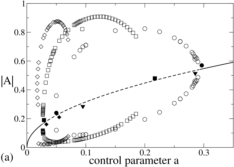
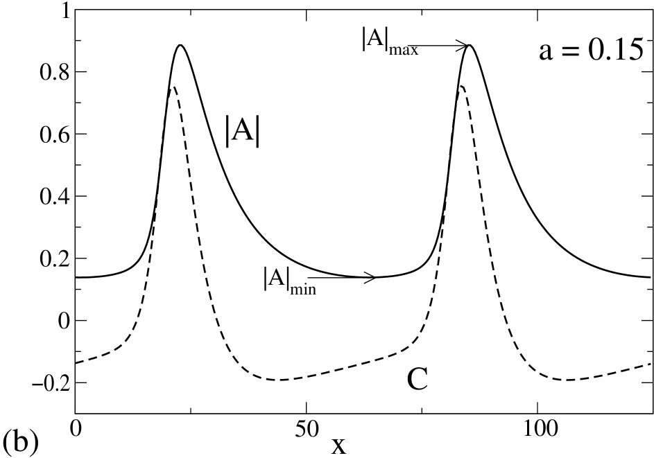
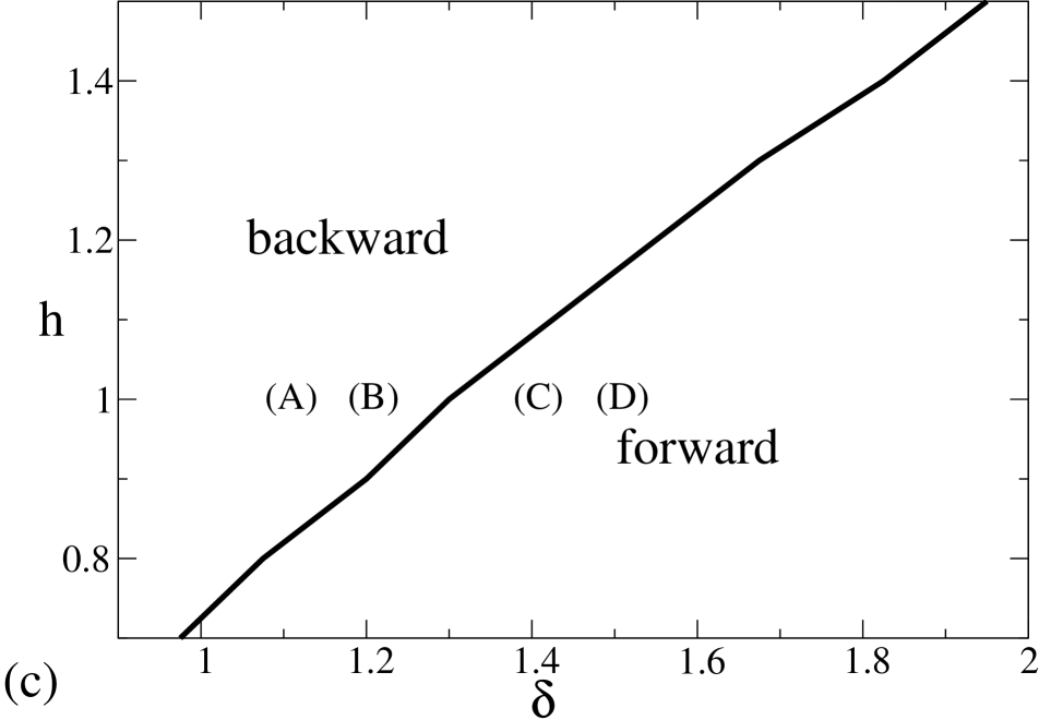
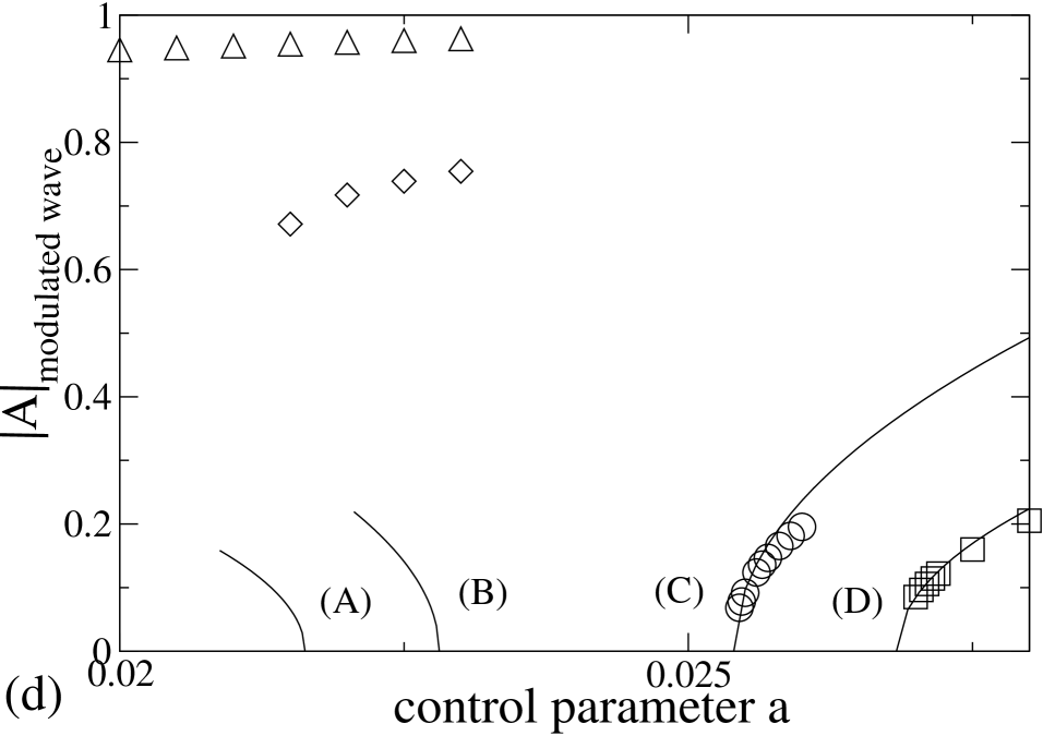
Figure 6: (a) Bifurcation diagram of modulated waves. Diamonds indicate minima and maxima of a single-wavelength modulation, squares and circles two and three wavelengths respectively. Solid symbols indicate the point at which the corresponding mode linearly destabilizes the traveling wave (triangles indicate four-wavelength instability although solution branches are not shown). Parameter values are s=1, h=1, $\delta$=1.5, $\alpha$=0.02 with a system size L=125. (b) Solution with 2-wavelength modulation. (c) Switch of the bifurcation from backward to forward according to (54). (d) Comparison of the results from the amplitude equation (solid lines) to numerical simulations confirms this transition. Enough data points where taken for (A),(B) to indicate the presence of bistability and thus confirm the subcritical nature of the bifurcations. s=1, h=1, $\alpha$=0.02, and $\delta$=1.1 (triangles),1.2 (diamonds),1.4 (circles),1.5 (squares) with a system size L=62.5.

and systematically arrive at a solvability condition at order O($\epsilon^{3}$) which yields a differential equation for $A_{0}$,

$$\partial_{\tau}A_{0}=\Lambda(a_{0},\alpha,\delta,h,s;p(a_{0},..))a_{2}A_{0}+\Pi(a_{0},\alpha,\delta,h,s;p(a_{0},..))|A_{0}|^{2}A_{0}.$$ (54)

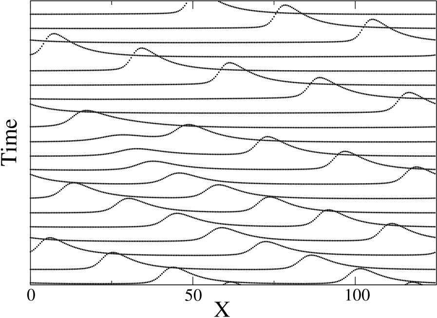
Figure 7: Space-time diagram of $|A|$ showing the annihilation of one ’hump’ by another leading to the formation of a single-wavelength modulated pattern from a two-wavelength pattern. s=1, h=1, $\alpha$=0.02, $\delta$=1.5, a=0.04

The coefficients $\Lambda$ and $\Pi$ in (54) must be solved numerically by determining the value of p from (50) for given values of the parameters. For the values of the parameters tested, it was found that the secondary bifurcation encountered first as the control parameter $a$ is increased from 0 can be either forward or backward (cf. stability island including a=0 in Fig. 5(a)). The bifurcation which occurs as $a$ is decreased from the region of stability of the plane waves was, in all cases, supercritical. A bifurcation diagram for the modulated waves is given in Figure 6(a) for a system size of L=125. The particular structure of the cascade of bifurcations is a consequence of the finite system size, where each branch corresponds to a discrete number of wavelengths of the modulation. The bifurcation to modulated waves near onset of the traveling waves (for small a) is examined in detail in Figures 6(c),(d) where the amplitude equation is compared to numerical simulation. As $\delta$ is decreased for fixed values of the other parameters, the bifurcation switches from forward to backward. Figure 6(d) confirms the validity of the amplitude equation.

The dynamics of the modulated wave pattern is not trivial. The destruction or creation of a modulation wavelength during the transient dynamics before the stable pattern is achieved occurs due to particle-like interactions of the ‘humps’ of the modulations as seen in Figure 7. The bifurcation diagram in Figure 6(a) indicates the existence of multiple branches for a single value of the control parameter. If the initial bifurcation is to a lower branch (say with 3 wavelengths), two of the three ’humps’ will collide after an initial periodically modulated state. The remaining two may again collide to form a single-wavelength modulation which is then stable.

As $\delta$ is decreased further, the subcritical branch of modulated waves, created in a saddle-node bifurcation as the control parameter is increased, extends further towards the onset of the traveling waves, eventually becoming bistable with the basic, conductive state (Fig. 8(a)). As in the supercritical case, the modulated-wave branches arise from an instability of the plane-waves to finite wavenumber modulations. Modulation wavenumbers $p$ which lie in the interval $p_{l}<p<p_{u}$, where the bounds depend on the value of the control parameter $a$, will linearly destabilize the plane-waves. For a finite system of length $L$, there will exist modulated-wave branches for all n such that $p=\frac{2n\pi}{L}$ lies in this interval. As $n$ is decreased the solutions increasingly take on the characteristics of localized objects (Fig. 8(b)). In fact, the distance between them can become arbitrarily large. Consequently, this distance can be much larger than the maximal wavelength $\frac{2\pi}{p_{l}}$ of modulations that linearly destabilize the traveling waves in a given system. Thus, these solutions do not bifurcate directly from the plane-wave branch but rather most likely arise in a tertiary bifurcation off a modulated-wave solution. For example, Figure 9 shows a series of modulated-wave branches for a system (L=250) where a single modulation (n=1) does not linearly destabilize the waves. Still, the single-pulse solution exists (dash-dot branch).

        

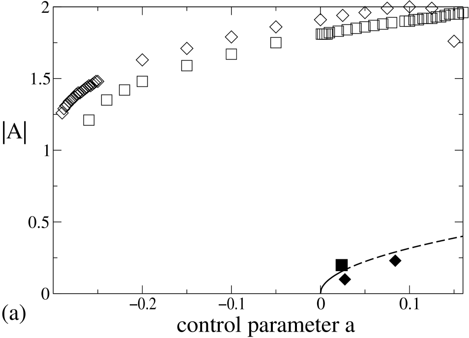
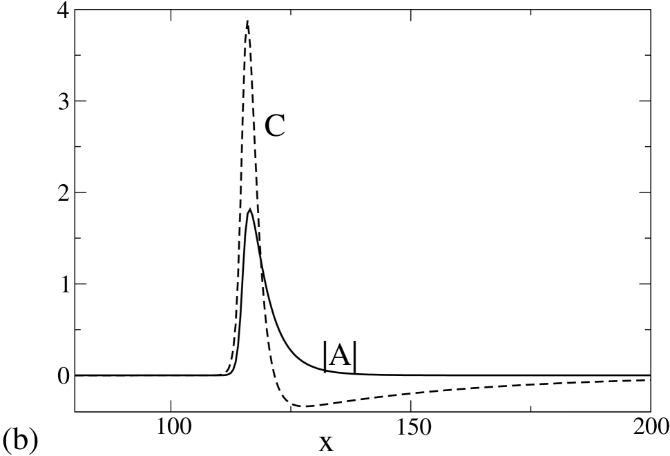
Figure 8: (a) Bifurcation diagram of pulses; the subcritical branch extends over the conductive state. The solid symbols indicate where the modes of the corresponding branches become linearly unstable. (b) Profile of the pulse solution with h=1, s=1, $\alpha$ = 0.02, $\delta$ = 0.5, a=-0.1. The solid line is the amplitude $|A|$ and the dashed line the C-field profile.

5 Conclusion

Systems similar to (3),(4) have been derived in various contexts, including a model of traveling interfacial waves in two-layer Couette flow [8] where $\alpha=0$ due to conservation of the additional zero-mode, given by the position of the interface. This system was shown to exhibit a phase-instability leading to a phase-slip [7] in agreement with experiment [1]. A small-amplitude model for traveling waves in thermal, binary-mixture convection consists of complex Ginzburg-Landau equations for counterpropagating waves coupled to a slowly decaying mode representing large-scale variations of the concentration field [4]. In this system the traveling waves arise in a backward bifurcation. Localized pulse solutions arising from instabilities of this system were identified and many of their properties characterized [16].

In this paper we have shown that the advected mode can cause the phase-instability to occur at finite wavelength and can introduce an additional amplitude-instability. The latter is identified as the origin of pulse-solutions seen in earlier works. They arise when the secondary bifurcation to modulated waves is sufficiently subcritical to lead to bistability between the modulated wave and the basic state. A similar bifurcation may explain the appearance of localized “worms” in electroconvection in nematic liquid crystals, seen again before the primary instability to supercritical traveling waves. Indeed, a model of traveling waves coupled to a slowly decaying field has been invoked to describe the worm dynamics, attaining qualitative agreement [14].

Finally, it would be worthwhile to consider the effect of dispersion in (4) on the dynamics discussed in this paper. In some cases dispersion has been shown to have a significant effect on the linear-stability properties of waves coupled to a additional mode. A model similar to (4, 5) used by Bartelet and Charru [1], with $\alpha=0$ and added dispersion, seems to explain qualitatively the linear-stability properties of waves observed in experiment. The inclusion of dispersion also allows for a determination of the effect of the additional mode on the Benjamin-Feir instability. In some cases this effect is important as, for example, in the 4-species Oregonator model [5] of the BZ reaction where the Benjamin- Feir instability can be preceded by a finite-wavenumber instability.

We would like to thank Blas Echebarria for many interesting and helpful discussions. This work was supported by the Engineering Research Program of the Office of Basic Energy Sciences at the Department of Energy (DE-FG02-92ER14303) and by a grant from NSF ((DMS 9804673).

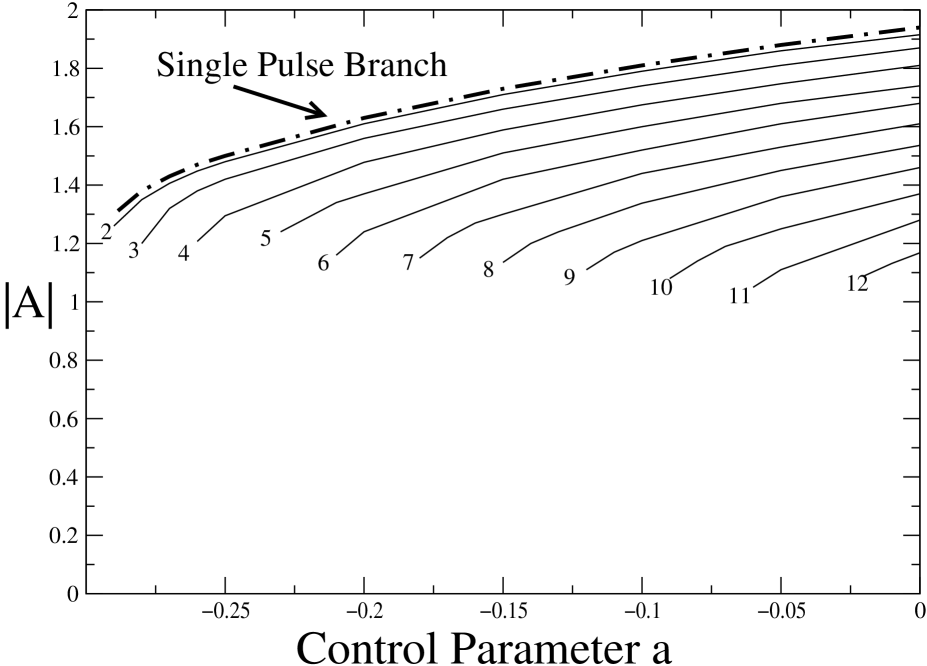
Figure 9: Bifurcation Diagram with $h$=1.0, $s$=1.0, $\alpha$=0.02, $\delta$=0.5, $q$=0 and L=250. Each branch represents a modulated-wave solution with the number of modulations given. As this number $n$ decreases, the modulated-waves become more like localized traveling pulses.

6 Appendix A: Derivation of Amplitude Equation for Phase Instability

Here we outline the derivation of the amplitude equation (44) which describes the slow-time evolution of modulations of plane waves in (20, 21). We consider finite-wavenumber modulations $p_{cr}$ of waves with wavenumber $q_{cr}$ as given by (40) and (39). We first expand the phase and C-field as,

$$\left(\begin{array}[]{cc}\phi\\ C\end{array}\right)=\left(\begin{array}[]{cc}q_{cr}X\\ 0\end{array}\right)+\epsilon\mathbf{\Phi_{0}}+\epsilon^{2}\mathbf{\Phi_{1}}+\dots,$$ (55)

where $\epsilon=\sqrt{\frac{a-a_{0}}{a_{2}}}$ and $a_{0}$ is the value of the control parameter at onset of the fastest-growing mode. We rewrite (20, 21) symbolically as,

$$\mathbf{\mathcal{L}}\left(\begin{array}[]{cc}\phi\\ C\end{array}\right)+\mathbf{\mathcal{N}}(\phi,C)=0,$$ (56)

and expand the linear and nonlinear operators in $\epsilon$,

$$\mathbf{\mathcal{L}} = L_{0}+\epsilon L_{1}+\epsilon^{2}L_{2}+\dots,$$ (57)

$$\mathbf{\mathcal{N}} = \epsilon^{2}N_{1}+\epsilon^{3}N_{2}+\dots,$$ (58)

$$D_{E} = D+\epsilon^{2}D_{2},$$ (59)

with

$$L_{0} = \left(\begin{array}[]{cc}D\partial_{X}^{2}-\partial_{T}&\frac{q_{cr}}{R^{2}}\partial_{X}\\ -2hq_{cr}\partial_{X}^{2}&\delta\partial_{X}^{2}-\partial_{T}-\alpha_{2}+(s+h)\partial_{X}\end{array}\right),$$ (62)

$$L_{1} = 0,$$ (63)

$$L_{2} = \left(\begin{array}[]{cc}D_{2}\partial_{X}^{2}-\partial_{\tau}&R_{2}\partial_{X}\\ 0&-\partial_{\tau}\end{array}\right),$$ (66)

$$N_{1} = \left(\begin{array}[]{cc}K_{1}C\partial_{X}^{2}\phi+K_{2}\partial_{X}\phi\partial_{X}^{2}\phi+K_{3}C\partial_{X}C+K_{4}\partial_{X}\phi\partial_{X}C,&-2h\partial_{X}\phi\partial_{X}^{2}\phi\end{array}\right)^{T},$$ (68)

$$N_{2} = \left(\begin{array}[]{cc}K_{5}\partial_{X}^{2}\phi(\partial_{X}\phi)^{2}+K_{6}C^{2}\partial_{X}^{2}\phi+K_{7}C\partial_{X}\phi\partial_{X}^{2}\phi+K_{8}(\partial_{X}\phi)^{2}\partial_{X}C+\\ K_{9}C\partial_{X}C\partial_{X}\phi+K_{10}C^{2}\partial_{X}C,&0\end{array}\right)^{T}.$$ (70)

where the coefficients are given by,

$$R = \sqrt{a_{0}-q_{cr}^{2}},R_{2}=-\frac{a_{2}q_{cr}}{R^{4}},$$ (72)

$$D = \frac{R^{2}-2q_{cr}^{2}}{R^{2}},D_{2}=\frac{a_{2}}{R^{2}}(1-D),$$ (73)

$$K_{1} = \frac{(1-D)}{R^{2}},K_{2}=\frac{2q_{cr}}{R^{2}}(D-3),$$ (74)

$$K_{3} = -\frac{q_{cr}}{R^{4}},K_{4}=\frac{1}{R^{2}}(1+\frac{2q_{cr}^{2}}{R^{2}}),$$ (75)

$$K_{5} = \frac{1}{R^{2}}(D-3-\frac{8a_{0}q_{cr}^{2}}{R^{4}}),K_{6}=-\frac{2q_{cr}}{R^{6}},$$ (76)

$$K_{7} = \frac{4q_{cr}}{R^{6}}(q_{cr}^{2}+a_{0}),K_{8}=\frac{q_{cr}}{R^{4}}(3+\frac{4q_{cr}^{2}}{R^{2}}),$$ (77)

$$K_{9} = -\frac{1}{R^{4}}(1+\frac{4q_{cr}^{2}}{R^{2}}),K_{10}=\frac{q_{cr}}{R^{6}}.$$ (78)

The slow time is given by $\tau=\epsilon^{2}T$. At order $\epsilon$ we recover the homogeneous, linearized system,

$$L_{0}\mathbf{\Phi_{0}}=0.$$ (79)

The zero-mode $\mathbf{\Phi_{0}}$ we take, as in 3.1, to be of the form,

$$\mathbf{\Phi_{0}}=\left(\begin{array}[]{cc}\Phi_{0}\\ C_{0}\end{array}\right)A_{0}(\tau)e^{i(p_{cr}X+\omega_{cr}T)}+c.c.$$ (80)

The eigenvector $(\Phi_{0},C_{0})^{T}$ is determined by solving (79),

$$\left(\begin{array}[]{cc}\Phi_{0}\\ C_{0}\end{array}\right)=\left(\begin{array}[]{cc}iq_{cr}\frac{p_{cr}}{R^{2}}\\ Dp_{cr}^{2}+i\omega_{cr}\end{array}\right)$$ (81)

The left-null eigenvector is found by solving the adjoint problem,

$$\mathbf{\Phi_{0}^{\dagger}}=\left(\begin{array}[]{cc}2hq_{cr}p_{cr}^{2}\\ Dp_{cr}^{2}-i\omega_{cr}\end{array}\right)e^{i(p_{cr}X+\omega_{cr}T)}.$$ (82)

At O($\epsilon^{2}$) we have

$$L_{0}\mathbf{\Phi_{1}}+N_{1}(\mathbf{\Phi_{0}})=0.$$ (83)

The nonlinear term $N_{1}$ contributes both spatio-temporally homogeneous modes and modes of twice the critical modulation. We thus take $\mathbf{\Phi_{1}}$ to be of the form,

$$\mathbf{\Phi_{1}}=\left(\begin{array}[]{cc}\Phi_{12}\\ C_{12}\end{array}\right)A_{0}^{2}e^{2i(p_{cr}X+\omega_{cr}T)}+c.c+\left(\begin{array}[]{cc}T\Phi_{10}\\ C_{10}\end{array}\right)|A_{0}|^{2}.$$ (84)

With this ansatz, (83) reduces to two linear, algebraic systems. The system corresponding to the forced second harmonic is

$$\left(\begin{array}[]{cc}-4Dp_{cr}^{2}-2i\omega_{cr}&2ip_{cr}\frac{q_{cr}}{R^{2}}\\ 8hq_{cr}p_{cr}^{2}&-4\delta p_{cr}^{2}-\alpha+2i(s+h)-2i\omega_{cr}\end{array}\right)\left(\begin{array}[]{cc}\Phi_{12}\\ C_{12}\end{array}\right)$$ (89)

$$+\left(\begin{array}[]{cc}K_{1}\Phi_{0}C_{0}p_{cr}^{2}+iK_{2}\Phi_{0}^{2}p_{cr}^{3}-iK_{3}C_{0}^{2}p_{cr}+K_{4}\Phi_{0}C_{0}p_{cr}^{2}\\ -2ih\Phi_{0}^{2}p_{cr}^{3}\end{array}\right)=0,$$ (92)

and that for the homogeneous forcing

$$\left(\begin{array}[]{cc}-1&0\\ 0&-\alpha\end{array}\right)\left(\begin{array}[]{cc}\Phi_{10}\\ C_{10}\end{array}\right)+\left(\begin{array}[]{cc}-K_{1}p_{cr}^{2}(\Phi_{0}^{*}C_{0}+\Phi_{0}C_{0}^{*})+K_{4}p_{cr}^{2}(\Phi_{0}^{*}C_{0}+\Phi_{0}C_{0}^{*})\\ 0\end{array}\right)=0.$$ (99)

Note that the homogeneous forcing causes a response in the phase which grows linearly with time, i.e. it changes the frequency of the wave (cf. (84)).

At O($\epsilon^{3}$) we have

$$L_{0}\mathbf{\Phi_{2}}+L_{2}\mathbf{\Phi_{0}}+\mathbf{N_{1}}(\mathbf{\Phi_{0},\Phi_{1}})+\mathbf{N_{1}}(\mathbf{\Phi_{1},\Phi_{0}})+\mathbf{N_{2}}(\mathbf{\Phi_{0},\Phi_{0},\Phi_{0}})=0.$$ (100)

At this order the critical Fourier mode appears through the nonlinear forcing terms and the action of the linear operator $L_{2}$ on the eigenvalue of the linearized operator of the original system. In order for a solution to exist, these contributions must lie orthogonal to the left nullspace of the operator $L_{0}$. We thus obtain the solvability condition,

$$\langle\mathbf{\Phi_{0}^{\dagger}}^{*},L_{2}\mathbf{\Phi_{0}}+\mathbf{N_{1}}(\mathbf{\Phi_{0},\Phi_{1}})+\mathbf{N_{1}}(\mathbf{\Phi_{1},\Phi_{0}})+\mathbf{N_{2}}(\mathbf{\Phi_{0}})\rangle=0,$$ (101)

where the inner product is defined as an integral over one period of the critical Fourier mode and the scalar product of the scalar vectors in $\Phi,C$-space. The solution of (101) results in a differential equation (44) for the complex amplitude $A_{0}$, the expression for which is extremely long and involved.

7 Appendix B: Derivation of Amplitude Equation at Bandcenter for Amplitude-Driven Instability

Here we follow the same procedure as in Appendix A in outlining the derivation of the Landau equation for the amplitude-driven instability. The calculation is carried out at bandcenter, i.e. $q=0$. We perturb the basic, plane-wave state in equations (47, 48) by expanding the real amplitude R and real field C in $\epsilon=\sqrt{\frac{a-a_{0}}{a_{2}}}$ where $a_{0}$ is defined as in Appendix A,

$$\left(\begin{array}[]{cc}R\\ C\end{array}\right)=\left(\begin{array}[]{cc}\sqrt{a_{0}}\\ 0\end{array}\right)+\epsilon\mathbf{\Psi_{0}}+\epsilon^{2}\mathbf{\Psi_{1}}+\dots.$$ (102)

We rewrite (47, 48) symbolically as,

$$\mathbf{\mathcal{L}}\left(\begin{array}[]{cc}R\\ C\end{array}\right)+\mathbf{\mathcal{N}}(R,C)=0.$$ (103)

We now expand the linear and nonlinear operators in $\epsilon$,

$$\mathbf{\mathcal{L}} = L_{0}+\epsilon L_{1}+\epsilon^{2}L_{2}+\dots,$$ (104)

$$\mathbf{\mathcal{N}} = \epsilon^{2}N_{1}+\epsilon^{3}N_{2}+\dots,$$ (105)

with

$$L_{0} = \left(\begin{array}[]{cc}\partial_{x}^{2}-\partial_{t}-2a_{0}&\sqrt{a_{0}}\\ 2h\sqrt{a_{0}}\partial_{x}&\delta\partial_{x}^{2}-\partial_{t}-\alpha+s\partial_{x}\end{array}\right),$$ (108)

$$L_{1} = 0,$$ (109)

$$L_{2} = \left(\begin{array}[]{cc}-2a_{2}-\partial_{\tau}&\frac{a_{2}}{2\sqrt{a_{0}}}\\ h\frac{a_{2}}{\sqrt{a_{0}}}\partial_{x}&-\partial_{\tau}\end{array}\right),$$ (112)

$$N_{1} = \left(\begin{array}[]{cc}RC-3\sqrt{a_{0}}R^{2},&2hR\partial_{x}R\end{array}\right)^{T},$$ (114)

$$N_{2} = \left(\begin{array}[]{cc}-R^{3},&0\end{array}\right)^{T}.$$ (116)

At order $\epsilon$ we recover the homogeneous, linearized system,

$$L_{0}\mathbf{\Psi_{0}}=0.$$ (118)

The zero-mode $\mathbf{\Psi_{0}}$ we take, as in 4.1, to be of the form,

$$\mathbf{\Psi_{0}}=\left(\begin{array}[]{cc}R_{0}\\ C_{0}\end{array}\right)A_{0}(\tau)e^{i(p_{cr}X+\omega_{cr}t)}+c.c.$$ (119)

The eigenvector $(R_{0},C_{0})^{T}$ is determined by solving (118),

$$\left(\begin{array}[]{cc}R_{0}\\ C_{0}\end{array}\right)=\left(\begin{array}[]{cc}\sqrt{a_{0}}\\ p_{cr}^{2}+i\omega_{cr}+2a_{0}\end{array}\right).$$ (120)

The left-null eigenvector is found by solving the adjoint problem,

$$\mathbf{\Psi_{0}^{\dagger}}=\left(\begin{array}[]{cc}-2h\sqrt{a_{0}}ip_{cr}\\ p_{cr}^{2}+2a_{0}-i\omega_{cr}\end{array}\right)e^{i(p_{cr}X+\omega_{cr}T)}.$$ (121)

At O($\epsilon^{2}$) we have

$$L_{0}\mathbf{\Psi_{1}}+N_{1}(\mathbf{\Psi_{0}})=0.$$ (122)

The nonlinear term $N_{1}$ contributes both spatio-temporally homogeneous modes and modes of twice the critical modulation. We thus take $\mathbf{\Psi_{1}}$ to be of the form

$$\mathbf{\Psi_{1}}=\left(\begin{array}[]{cc}R_{12}\\ C_{12}\end{array}\right)A_{0}^{2}e^{2i(p_{cr}X+\omega_{cr}T)}+c.c+\left(\begin{array}[]{cc}R_{10}\\ C_{10}\end{array}\right)|A_{0}|^{2}.$$ (123)

With this ansatz, (122) reduces to two linear, algebraic systems. The system corresponding to the forced second harmonic is

$$\left(\begin{array}[]{cc}-4p_{cr}^{2}-2i\omega_{cr}-2a_{0}&\sqrt{a_{0}}\\ 4h\sqrt{a_{0}}ip_{cr}&-4\delta p_{cr}^{2}-2i\omega_{cr}-\alpha+2isp_{cr}\end{array}\right)\left(\begin{array}[]{cc}R_{12}\\ C_{12}\end{array}\right)$$ (128)

$$+\left(\begin{array}[]{cc}R_{0}C_{0}-3\sqrt{a_{0}}R_{0}^{2}\\ 2ihp_{cr}R_{0}^{2}\end{array}\right)=0,$$ (131)

and that for the homogeneous forcing

$$\left(\begin{array}[]{cc}-2a_{0}&\sqrt{a_{0}}\\ 0&-\alpha\end{array}\right)\left(\begin{array}[]{cc}R_{10}\\ C_{10}\end{array}\right)+\left(\begin{array}[]{cc}R_{0}C_{0}^{*}+R_{0}^{*}C_{0}-6\sqrt{a_{0}}|R_{0}|^{2}\\ 0\end{array}\right)=0.$$ (138)

Solving these systems yields the following expression for the scalar quantities,

$$R_{12} = \frac{m_{12}}{d_{12}},$$ (139)

$$C_{12} = \frac{n_{12}}{d_{12}},$$ (140)

$$m_{12} = -\frac{1}{2}\sqrt{a_{0}}(4a_{0}\delta p_{cr}^{2}+4\delta p_{cr}^{4}+a_{0}\alpha+p_{cr}^{2}\alpha+2\omega_{cr}sp_{cr}-2\omega_{cr}^{2}+i[4\delta p_{cr}^{2}\omega_{cr}$$ (141)

$$+\alpha\omega_{cr}-2a_{0}sp_{cr}-2sp_{cr}^{3}+2a_{0}\omega_{cr}+2\omega_{cr}p_{cr}^{2}+2a_{0}hp_{cr}]),$$

$$n_{12} = -4a_{0}hp_{cr}\left(-\omega_{cr}+i[a_{0}+\frac{3}{2}p_{cr}^{2}]\right),$$ (142)

$$d_{12} = -8\delta p_{cr}^{4}-2(\alpha+2a_{0}\delta)p_{cr}^{2}-a_{0}\alpha+2\omega_{cr}(\omega_{cr}-sp_{cr})$$ (143)

$$i[4sp_{cr}^{3}-4\omega_{cr}(1+\delta)p_{cr}^{2}+2a_{0}p_{cr}(s+h)-\omega_{cr}(2a_{0}+\alpha)],$$

$$R_{10} = -\sqrt{a_{0}}+\frac{1}{\sqrt{a_{0}}}(p_{cr}^{2}+2a_{0}),$$ (144)

$$C_{10} = 0.$$ (145)

At cubic order projection onto the left null eigenvector yields the amplitude equation for $A_{0}$,

$$\partial_{\tau}A_{0} = l(p_{cr})(p_{cr}^{2}+i\omega_{cr})A_{0}+l(p_{cr})\sqrt{a_{0}}$$ (146)

$$[C_{12}\sqrt{a_{0}}-3a_{0}^{3/2}+2R_{12}(p_{cr}^{2}-a_{0})+2R_{10}(p_{cr}^{2}-a_{0}+i\omega_{cr})]|A_{0}|^{2}A_{0},$$

$$l(p_{cr}) = 2ihp_{cr}\frac{\{(p_{cr}^{2}+2a_{0})^{2}-\omega_{cr}^{2}-2i[\omega_{cr}(p_{cr}^{2}+2a_{0})+ha_{0}p_{cr}]\}}{[(p_{cr}^{2}+2a_{0})^{2}-\omega_{cr}^{2}]^{2}+4[\omega_{cr}(p_{cr}^{2}+2a_{0})+ha_{0}p_{cr}]^{2}}.$$ (147)

References

[1]
F. Charru and P. Barthelet.
Secondary instabilities of interfacial waves due to coupling with a
long wave mode in a two-layer Couette flow.
Physica D, 125:311, 1999.
[2]
B.A. Malomed.
Patterns produced by a short-wave instability in the presence of a
zero mode.
Phys. Rev. A, 45:1009, 1992.
[3]
H. Riecke.
Self-trapping of traveling-wave pulses in binary mixture convection.
Phys. Rev. Lett., 68:301, 1992.
[4]
H. Riecke.
Ginzburg-Landau equation coupled to a concentration field in
binary-mixture convection.
Physica D, 61:253–259, 1992.
[5]
M. Ipsen and P.G. Soerensen.
Finite wavelength instabilities in a slow mode coupled complex
ginzburg-landau equation.
Phys. Rev. Lett., 84:2389–2392, 2000.
[6]
P.C. Matthews and S.M. Cox.
Pattern formation with a conservation law.
Nonlinearity, 13:1293–1320, 2000.
[7]
P. Bartelet and F. Charru.
Benjamin-feir and eckhaus instabilities with galilean invariance: the
case of interfacial waves in viscous shear flows.
Eur. J. Mech., B/Fluids, 17:1–18, 1998.
[8]
M. Renardy and Y. Renardy.
Derivation of amplitude equations and analysis of sideband
instabilities in two-layer flows.
Phys. Fluids, 5:2738, 1993.
[9]
A. Bernoff.
Finite amplitude convection between stress-free boundaries;
ginzburg-landau equations and modulation theory.
Euro. J. Appl. Math., 5:267, 1994.
[10]
E.D. Siggia and A. Zippelius.
Pattern selection in Rayleigh-Béard convection near threshold.
Phys. Rev. Lett., 47:835, 1981.
[11]
F.H.Busse and E.W.Bolton.
Instabilities of convection rolls with stress-free boundaries near
threshold.
J.Fluid Mech., 146:115–125, 1984.
[12]
P. Kolodner.
Drifting pulses of traveling-wave convection.
Phys. Rev. Lett., 66:1165, 1991.
[13]
W. Barten, M. Lücke, and M. Kamps.
Localized traveling-wave convection in binary fluid mixtures.
Phys. Rev. Lett., 66:2621, 1991.
[14]
H. Riecke and G.D. Granzow.
Localization of waves without bistability: Worms in nematic
electroconvection.
Phys. Rev. Lett., 81:333, 1998.
[15]
M. Dennin, G. Ahlers, and D.S. Cannell.
Chaotic localized states near the onset of electroconvection.
Phys. Rev. Lett., 77:2475, 1996.
[16]
H. Riecke.
Solitary waves under the influence of a long-wave mode.
Physica D, 92:69–94, 1996.
[17]
C. Martel and J.M. Vega.
Dynamics of a hyperbolic system that applies at the onset of the
oscillatory instability.
Nonlinearity, 11:105, 1998.