Outliers, Extreme Events and Multiscaling

Abstract

Extreme events have an important role which is sometime catastrophic in a variety of natural phenomena including climate, earthquakes and turbulence, as well as in man-made environments like financial markets. Statistical analysis and predictions in such systems are complicated by the fact that on the one hand extreme events may appear as “outliers” whose statistical properties do not seem to conform with the bulk of the data, and on the other hands they dominate the (fat) tails of probability distributions and the scaling of high moments, leading to “abnormal” or “multi”-scaling. We employ a shell model of turbulence to show that it is very useful to examine in detail the dynamics of onset and demise of extreme events. Doing so may reveal dynamical scaling properties of the extreme events that are characteristic to them, and not shared by the bulk of the fluctuations. As the extreme events dominate the tails of the distribution functions, knowledge of their dynamical scaling properties can be turned into a prediction of the functional form of the tails. We show that from the analysis of relatively short time horizons (in which the extreme events appear as outliers) we can predict the tails of the probability distribution functions, in agreement with data collected in very much longer time horizons. The conclusion is that events that may appear unpredictable on relatively short time horizons are actually a consistent part of a multiscaling statistics on longer time horizons.

I Introduction

There is an obvious and wide spread interest in predicting extreme events in a variety of contexts. Particularly well known examples are the insurance risks related to large tropical storms, human and property risks in the context of large earthquakes, financial risks caused by large movements of the markets, and dangers to passenger planes due to extremely intermittent turbulent air velocities. Obviously, any improvement in the predictability of any of these extreme events is highly desirable for a number of reasons. Accordingly, there exists a large body of work focusing on the statistics of such events, small, intermediate and large, with the aim of studying the ensuing probability distribution functions (PDF). If one can model properly the PDF, one can in principle predict at least the frequency of extreme events. Yet, there is one fundamental question that arises that needs to be confronted first: are the extreme events sharing the same statistical properties as the small and intermediate events, or are they ”outliers”? If the latter is true, then no analysis of the core of the PDF, clever as it may be, could yield a proper answer to the desire to predict the probability of extreme events.

Indeed, in a number of context it had been proposed recently that extreme events are “outliers” [1]. For example in financial markets the largest draw-downs appear to exhibit properties that differ from the bulk of the fluctuations [2]. In general one would refer to “outliers” when the rate of occurrence of small and intermediate events lies on a PDF with some given properties, while the extreme events appear to exhibit statistical properties that differ from the bulk in a significant way. The aim of this paper is to present a detailed analysis of the fluctuations in a turbulent dynamical system that shows that such a point of view can be substantiated . Clearly, this type of considerations must be conducted with great care. The danger is that on small time horizons the largest events appear so rarely, once or twice, that their rate of occurrence is not statistically significant, and no conclusion about their relation to the statistics of small and intermediate events is possible. Nevertheless, we offer in this paper a positive outlook. We will show that in the context of the bulk of this paper, which is the analysis of a shell model of turbulence, one can analyze within the short time horizon the dynamics of the extreme events. This analysis reveals their special dynamical scaling properties, allowing us to make interesting predictions about the tails of the distribution functions even before the full statistics is available. These predictions can be checked in our case by considering much longer time horizons. The conclusion for the extreme events community is that it may very well pay to look very carefully at the detailed dynamics of the extreme events if one wants to claim anything about their probability of occurrence.

The model that we treat in detail in this paper is a so-called “shell” model of turbulence. Shell models of turbulence [3, 4, 5, 6, 7, 8] are simplified caricatures of the equations of fluid mechanics in wave-vector representation; typically they exhibit anomalous scaling even though their nonlinear interactions are local in wavenumber space. The wavenumbers are represented as shells, which are chosen as a geometric progression

$$k_{n}=k_{0}\lambda^{n}\,,$$ (1)

where $\lambda$ is the “shell spacing”. There are $N$ degrees of freedom where $N$ is the number of shells. The model specifies the dynamics of the “velocity” $u_{n}$ which is considered a complex number, $n=1,\dots,N$. Their main advantage is that they can be studied via fast and accurate numerical simulations, in which the values of the scaling exponents can be determined very precisely. We employ our own home-made shell model which had been christened the Sabra model[8]. It exhibits similar anomalies of the scaling exponents to those found in the previously popular GOY model [3, 4], but with much simpler correlation properties, and much better scaling behavior in the inertial range. The equations of motion for the Sabra model read:

$$\frac{du_{n}}{dt} = i\big{(}ak_{n+1}u_{n+2}u_{n+1}^{*}+bk_{n}u_{n+1}u_{n-1}^{*}$$ (3)

$$-ck_{n-1}u_{n-1}u_{n-2}\big{)}-\nu k_{n}^{2}u_{n}+f_{n}\,,$$

where the star stands for complex conjugation, $f_{n}$ is a forcing term which is restricted to the first shells and $\nu$ is the “viscosity”. In this paper we restrict the forcing to the first and and second shells only ($n=1,2)$. The coefficients $a,b$ and $c$ are chosen such that

$$a+b+c=0\ .$$ (4)

This sum rule guarantees the conservation of the “energy”

$$E=\sum_{n}|u_{n}|^{2}\,,$$ (5)

in the inviscid ($\nu=0$) limit.

The main attraction of this model is that it displays multiscaling in the sense that moments of the velocity depend on $k_{n}$ as power laws with nontrivial exponents:

$$S_{p}(k_{n})\equiv\langle|u_{n}|^{p}\rangle\propto k_{n}^{-\zeta_{p}}\propto\lambda^{-n\zeta_{p}}\,,$$ (6)

where the scaling exponents $\zeta_{p}$ exhibit non linear dependence on $p$. We expect such scaling laws to appear in the “inertial range” with shell index $n$ larger than the largest shell index that is effected by the forcing, denoted as $n_{L}$, and smaller than the shell indices affected by the viscosity, the smallest of which will be denoted as $n_{d}$. The scaling exponents were determined with high numerical accuracy better than $0.02$ in Ref.[8].

To introduce the issue behind the title of this paper, we present in Fig. 1 a typical time series for $u_{11}$. The parameters of the model are detailed in the figure legend. One can see the typical appearance of rare events with amplitude that exceeds the mean by a factor of 6–8. To pose the question in its clearest way we display in Fig. 2 a distribution function which is the normalized rate of occurrence (i.e. the number of times) that a given amplitude has been observed in the time window of $10^{7}$ time steps. This apparent relative frequency of events is very similar to findings in real data, see for example Fig. 1 of Ref. [2]. which deals with draw downs in the Dow Jones Average. Similarly to the analysis there, we can pass an approximate straight line through the points representing small and intermediate events. Such an exponential law would mean that the events of $|u_{11}|^{2}$ with amplitudes larger than, say, 4$\langle|u_{11}|^{2}\rangle$ are clear outliers. Their probability is so low that they should not have appeared in the short time horizon at all. We could conclude, like in the analysis of Ref. [2], that the extreme events cannot be dealt with the same distribution function as the small and intermediate events.

FIG. 1.: Time series for normalized velocity of the 11th shell. Parameters of the numerics: $a=1$, $b=c=-0.5$, $\lambda=2$, $N=28$, $k_{0}=1/64$, time correlated random forcing on the first two shells with characteristic amplitude $0.005(1+i)$. Decorrelation time is chosen about turnover time of the 1st shell.

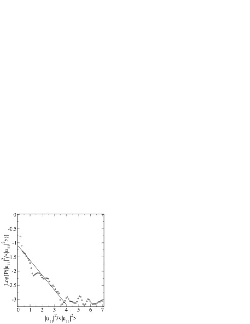
FIG. 2.: Apparent probability distribution function for 11th shell. Averaging over $10^{7}$ time-steps which is about 250 decorrelation times for this shell. The data contains additional, extremely sparse events of amplitude larger than 7, occurring once each; these were left out in this plot.

On the other hand, it is very possible that the low rate of occurrence of the extreme events in Fig. 2 means simply that they are statistically irrelevant and that no conclusion can be drawn. How to overcome this difficulty? The purpose of this paper is to show that indeed the extreme events may have dynamical scaling properties that are all their own, and that they affect crucially the tails of the distributions functions, making them very broad indeed. The main new point is that detailed analysis of the extreme events in the short time horizon suffices to make lots of predictions about the tails of the PDF’s, predictions that in our case can be easily confirmed by considering much longer time horizons.

In explaining our ideas we will try to distinguish aspects which are general, and that in our view may have applications to other systems with extreme events, and aspects which are particular to the example of the shell model of turbulence. Thus we start in Sect.2 with an analysis of the temporal shape of the extreme events. We believe that this analysis is very general, leading to an important relation between the amplitude of the event and its time scale (the time elapsing from rise up to demise). In Sect. 3 we employ the dynamical scaling form of the extreme events to present a theory of the tails of the distribution functions. We can relate the tails of PDF’s belonging to different scales. In Sect. 4 we discuss numerical studies of the PDF’s, distinguishing the core and the tails. In Sect.5 the main numerical findings are rationalized theoretically on the basis of universal “pulse” solutions of the dynamics of the Sabra model. Section 6 contains the bottom line: we make use of the scaling relations to predict the tails of PDF’s from data collected within short time horizons. Direct measurements of these tails give nonsense unless the time horizons are increased a hundred fold. Yet with the help of the theoretical forms we can offer predicted tails that agree very well with the data collected with much longer time horizons.

II Detailed dynamics and scaling of the extreme events

In turbulence in general and in our shell model in particular the energy that is injected by the forcing at the largest scales ($n=1$ and 2) is transferred on the average to smaller scales. It is advantageous to analyze the extreme events of a given scale (or given shell $n$) and also to follow the cascade of extreme events from scale to scale. We first consider a given shell.

A Temporal dependence of extreme events of a given scale

We focus here on the detailed dynamics of the largest events of a given scale. We considered for example the time series of the 20th shell ($n=20$) and isolated the 5 largest events (in terms of their amplitude) as they occurred in a time window of $10^{7}$ time steps. In the first step of analysis we normalized these 5 events by the amplitude at their maximum. Next we plotted these normalized events as a function of time, subtracting the time at which they have reached their maximum value. The result of this replotting is shown in Fig. 3. Obviously a similar replotting can be done for any time series, and by itself is contentless.

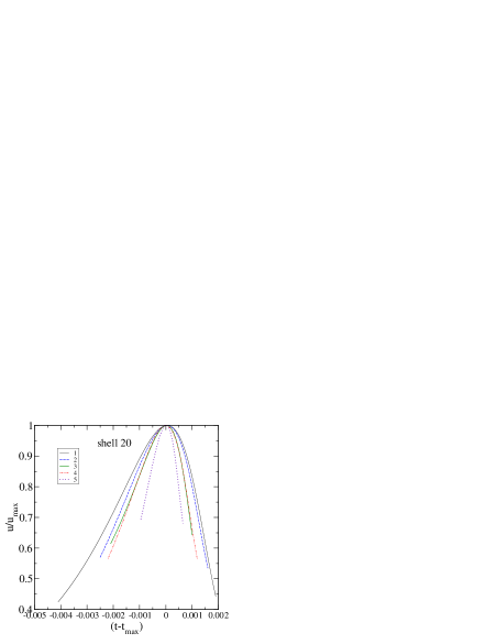
FIG. 3.: Collapse (of positions and amplitudes) for five intensive peaks belonging to 20th shell. The values of $u_{\rm max}$ for the peaks numbered from 1 to 5 are 4.65, 4.77, 6.71, 7.40 and 10.5 respectively, in units of the rms velocity in this shell. The narrowest peak is thus the tallest.

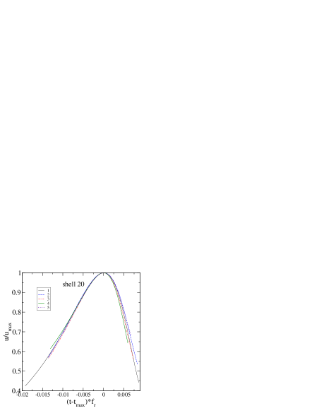
FIG. 4.: Full collapse (of the position, amplitude and width) of the same as in Fig. 3 peaks. The ordering of the points is 1 to 5 from left to right.

The next step of analysis will reveal already something interesting. Building on the normalized events of Fig. 3 we attempt to rescale the time axis for each event in order to collapse the data together. Of course, each event calls for a different rescaling factor, which we denote (in frequency units) as $f_{r}$. The fact that such a rescaling factors exist, and that they leads to data collapse as shown in Fig. 4, is a not trivial fact which may or may not exist in different cases. But we will show that if such a rescaling is found, it can serve as a starting point for very useful considerations.

The third step of the present analysis is a search of meaning to the rescaling factors $f_{r}$. We hope that $f_{r}$ has a simple relation to the amplitude of the extreme events. To test this we can plot the individual values of $f_{r}$ found in Fig. 4 as a function of the amplitude at the peak. The resulting plot is shown as Fig. 5. In passing the straight line through the data points we included the point $(0,0)$ in the analysis, as we search for a simple scaling form

$$f_{r}\propto u_{\rm max}^{x}\ .$$ (7)

with $x$ a scaling exponent. We conclude that in this case we have a satisfactory scaling law with $x=1$.

The meaning of this scaling law is quite apparent in the present case. Looking back at the equation of motion we realize that from the point of view of power counting (not to be confused with actual dynamics) it can be written as

$$\frac{du}{dt}\propto u^{1+x}$$ (8)

with $x=1$. It is thus acceptable that a rescaling of $1/t$ by $u_{\rm max}$ should collapse all the extreme events as shown above. If the equation of motion were cubic in $u$ we could expect $x=2$ etc. Obviously, the rescaling analysis in this case revealed the type of dynamics underlying the process. Whether this can be done effectively in other case where extreme events are crucial is an open question for future research.

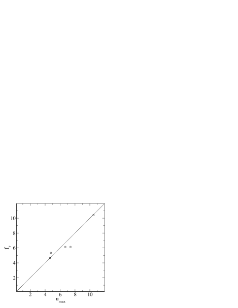
FIG. 5.: Width normalization vs amplitude for 5 peaks collapsed on Fig. 4.

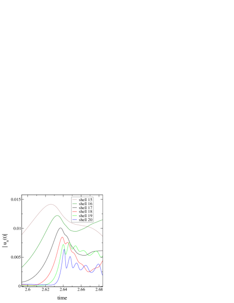
FIG. 6.: “Evolution” of a peak from the 15th to the 20th shell. The amplitudes are all in the same (arbitrary) units. One sees a progressive shift of the maximum to the right and a decrease in the amplitude, accompanied by narrowing and splitting. Nevertheless the form of the central part of the peak remains self-similar as exempified in the two following figures.

B Transfer of extreme events between different scales

To gain further understanding of the extreme events we focus now on the transfer from scale to scale. Consider for example a particular large amplitude event in the shell $n=15$, and its future fate as time proceeds. This is shown in Fig. 6. The event reached its highest amplitude at shell 15 around $t=2.625$. At a slightly later time it appeared as a large event in shell 16, and with a shorter delay at shell 17 where it started to split into a doublet. At even shorter delays this event emerges as a triplet and a multiplet at shells 18,19 and 20 respectively.

A very important characteristic of the dynamics of large events can be obtained from finding how to relate the maximal amplitudes of the first peak in the different shells. As was done above, we first replot all the first peaks as a function of time minus the time $t_{n}$ of their maximal amplitude $u_{n,\rm max}$. We then glue all the maxima together by rescaling the peaks amplitudes relative to the peak of a chosen shell. Denote by $K_{\rm am}(n,m)$ the relative amplitude of the peak in the $n$th shell to the $m$th shell. Choosing in our example $m=20$ we then seek a single exponent $y$ such that

$$K_{\rm am}(n,20)\equiv u_{n,\rm max}/u_{20,\rm max}=\lambda^{(20-n)y}\,,$$ (9)

where $\lambda$ is the shell spacing defined by Eq. (1). The value of $y$ is obtained by plotting $g_{\rm am}(n)$ vs $(20-n)$ where

$$g_{\rm am}(n)\equiv\ln[K_{\rm am}(n,20)]/\ln\lambda=y\,(20-n)\ .$$ (10)

The best fit is obtained with $y=0.24\pm 0.01$, see Fig. 9. The peaks which are now glued at their maxima as shown in Fig. 7 still have very different time-width.

Next, as before, we want to collapse all these curves by rescaling the time axis according to $(t-t_{n})\to(t-t_{n})/K_{\rm w}(n,20)$. Expecting the scaling law $K_{\rm w}(n,20)=\lambda^{z(20-n)}$ it is natural to consider

$$g_{\rm w}(n)\equiv\ln[K_{\rm w}(n,20)]/\ln\lambda=z\,(20-n)\ .$$ (11)

The exponent $z=0.75\pm 0.02$ is found by computing “the best” linear fit of $g_{\rm w}(n)$ vs $(20-n)$, see Fig. 9. The quality of the resulting data collapse can be seen in Fig. 8. Note, that within the error bars $z+y=1$. This sum rule will be rationalized theoretically in Sec. V.

The bottom line of this analysis can be summarized in a dynamical scaling form for the extreme events:

$$u_{n}(t)\approx v\lambda^{-yn}f\left[(t-t_{n})vk_{0}\lambda^{zn}\right]\ .$$ (12)

Here $v$ is a characteristic velocity amplitude associated with the cascade of a particular large event which starts at small $n$ and reaches eventually large values of $n$. As such $v$ is not universal. We stress that the scaling form was derived on the basis of a time series in the short time horizon, i.e. the the same one that gave rise to the apparent PDF shown in Fig. 1. We will see that these findings suffice to make rather strong predictions about the expected form of the converged PDF. A theoretical understanding of the origin of the scaling form (12) will be presented in Sec. V.

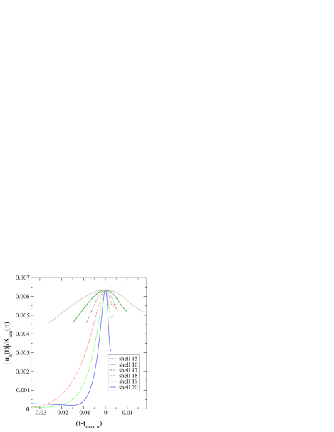
FIG. 7.: Collapse of the peak amplitudes for 15–20 shells. Initial peaks are shown on Fig. 6.

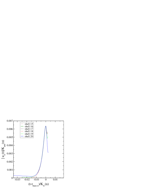
FIG. 8.: Full self-similar collapse of the peaks for 15–20 shells.

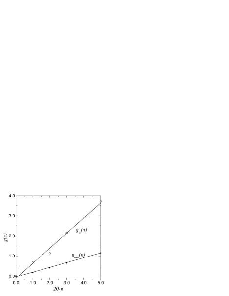
FIG. 9.: Fits of the rescaling factors $g_{\rm w}(n)$ and $g_{\rm am}(n)$ for the peaks in the shells 15 – 20 shown in Figs. 6,7 and 8. Note that in comparing different shells the rescaling of the frequency increases when the peak decreases in amplitude. This is opposite to the rescaling of peaks within a given shell.

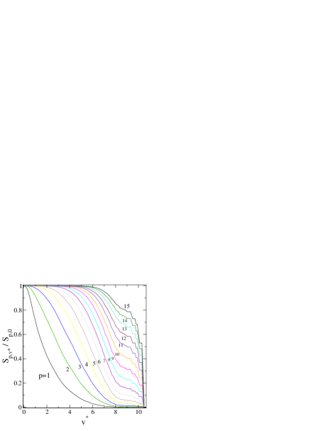
FIG. 10.: Normalized contributions to the structure functions of orders $p=1,\ 2\ \dots 15$ for 20th shell from the part of the velocity realization with $v>v_{*}$

III Implications for the tails of the Probability Distribution Functions

A Asymptotic Scaling Exponents

Having a scaling form for the large events means a great deal for the structure functions $S_{p}(k_{n})$ [cf. Eq. (6)] for high values of $p$. In fact for high $p$ the structure functions are dominated by the large events. To demonstrate this we show in Fig. 10 the relative contribution to $S_{p}(k_{20})$ that arise from velocity amplitudes that exceed a threshold $v_{*}$. In this plot $S_{p,v_{*}}$ is the structure function Eq. (6) where only events with $u_{20}\geq v_{*}$ are considered, whereas $S_{p,0}$ contains all the data. Obviously the higher $p$ is the higher is the contribution of large events. For any time window there exists the largest event, and when $v_{*}$ exceeds its value, $S_{p,v_{*}}$ necessarily vanishes.

If we accept the scaling form (12) we can use it to predict the scaling exponent $\zeta_{p}$ for high values of $p$. By definitions

$$S_{p}(k_{n})=\lim_{T\to\infty}\frac{1}{2T}\int\limits_{-T}^{T}|u_{n}|^{p}dt\propto k_{n}^{-\zeta_{p}}\propto\lambda^{-n\zeta_{n}}\ .$$ (13)

For $p$ large enough the structure functions are dominated by the well separated events. Instead of the integral in the interval $[-T,T]$ we can sum up the inegrals over the separated peaks. Substituting for each peak the form  (12) and noting that the number of peaks is proportional to $T$, we can extend the integration interval to $[-\infty,\infty]$ and write

$$S_{p}(k_{n}) \propto \lambda^{-ynp}\!\!\int\limits_{-\infty}^{\infty}\!\!f^{p}(\lambda^{zn}tvk_{0})dt$$ (14)

$$\propto \lambda^{-n(yp+z)}\!\!\int\limits_{-\infty}^{\infty}\!\!f^{p}(\tau)d\tau\ .$$ (15)

Comparing the exponents of $\lambda$ here and in the previous equation we find the scaling exponents

$$\zeta_{p}=yp+z\ .$$ (16)

Of course this prediction is valid only for high values of $p$ for which the contributions of the isolated peaks are domninant.

B Tails of the Probability Distribution Function

We turn now to the prediction of the tails of the PDFs assuming that these tails are dominated by well separated peaks with self-similar evolution (12). We will see below [and cf. Eq. (21)], that the tails of the predicted PDF are very sensitive to the exponents in Eq. (12), but rather insensitive to the precise form of the universal function $f(x)$ in Eq.(14). Assume then for simplicity that $f(x)=1$ for $|x|\leq 1/2$ and $f(x)=0$ for $|x|>1/2$. There is the free parameter $v$ in Eq. (12); for the chaotic realizations $u_{n}(t)$ we consider it as a random parameter. Define then the variable $V^{2}$ according to

$$V^{2}\equiv v^{2}/v_{0}^{2}\,,\quad v_{0}^{2}=\sum_{n=1}^{\infty}\langle u_{n}^{2}\rangle\ .$$ (17)

Consider now a run with a total time horizon $T\equiv 1/(k_{0}v_{0})$. Denote as $W(V^{2})dV^{2}$ the number of peaks measured in this run in which the value of $V^{2}$ fell in the window $[V^{2},(V^{2}+dV^{2})]$.

Next denote normalized amplitudes [the value of the signal at times $t=t_{n}$ in Eq.(12)]

$$U_{n}^{2}\equiv\frac{u_{n}^{2}}{\langle u_{n}^{2}\rangle}=\frac{V^{2}}{C\lambda^{\alpha n}}\,,\quad\alpha\equiv 2y-\zeta_{2}\,,$$ (18)

where $C$ is a dimensionless constant. We are interested in the PDF $P_{n}(U_{n}^{2})$, where $P_{n}(U_{n}^{2})dU_{n}^{2}$ is the probability to sample a normalized amplitude in the $n$th shell between $U_{n}^{2}$ and $U_{n}^{2}+dU_{n}^{2}$. By definition, the number of observations of such amplitudes in the time horizon $T$ is $dN_{n}$

$$dN_{n}=P_{n}(U_{n}^{2})dU_{n}^{2}\frac{T}{\tau_{0}}\ ,$$ (19)

where $\tau_{0}$ is the length of the sampling intervals. On the other hand, since the lifetime of a peak with a given value of $V^{2}$ belonging to the $n$th shell is $1/vk_{0}\lambda^{zn}$, we can also estimate the number of observations $dN_{n}$ as

$$dN_{n}=\frac{W(V^{2})}{\tau_{0}vk_{0}\lambda^{nz}}dV^{2}\ .$$ (20)

Equating Eqs.(19) and (20) and rearranging, one gets:

$$P_{n}(U_{n}^{2})=C\,W(V^{2})\lambda^{n(\alpha-z)}/V\ .$$ (21)

This relation is obtained under the assumption that the number of peaks is not increasing in the cascade process. In fact we saw that the number of the peaks is increasing with the shell number $n$, presumably in a scale-invariant manner as $\lambda$ to some positive exponent $\beta$. We can account for this effect by replacing in Eq. (21) $W$ by $\lambda^{\beta}\,W$. After that:

$$P_{n}(U_{n}^{2})=C\,W(V^{2})\lambda^{n(\alpha+\beta-z)}/V\,,$$ (22)

where $V^{2}$ and $U_{n}^{2}$ are defined by Eqs. (17) and (18). Equation (22) means that a collapse of the tails of the PDFs for different shells may be achieved by rescaling the $x$-axis $U_{n}^{2}\to V^{2}$ according to (18) and rescaling of the PDFs ($y$-axis) by $\lambda^{n(\alpha+\beta-z)}$.

Equation (22) for the tail of the PDFs allows one to find the high order structure functions (which are dominated by the tails of the PDFs) and their scaling exponents $\zeta_{p}$:

$$S_{p}(k_{n}) = \int\limits_{0}^{\infty}u_{n}^{p}P_{n}(U_{n}^{2})\,d\,U_{n}^{2}=C_{p}\,v_{0}^{p}\,\lambda^{n(\beta-z-yp)}\,,$$ (23)

$$C_{p} = \int\limits_{0}^{\infty}V^{p-1}W(V^{2})\,\,V^{2}\ .$$ (24)

Comparing again the exponents of $\lambda$ here and in Eq.(13) gives the prediction for the high order scaling exponents:

$$\zeta_{p}=yp+z-\beta\,,$$ (25)

which coincides with Eq. (16) at $\beta=0$. One sees that the effect of peak splitting (which was described by positive exponent $\beta$) increases the deviation of the scaling exponents from its K41 value $\zeta_{p}=p/3$.

IV Numerical studies of the PDF: core and tail

It is well known that PDF’s in multiscaling systems are not scale invariant. Nevertheless we need to examinte the possibility that the cores of the PDF’s can be collapsed using a rescaling law that is charateristic to them, while the tails may be collapsed using another rescaling law (with different scaling exponents). This possibility is related to the fact that the structure functions $S_{p}(k_{n})$ have scaling exponents in the vicinity of the K41 values ($\zeta_{{}_{\rm K41}}(p)=p/3$) for $p$ small enough, [say $p\leq 6$]. For large value of $p$ (say $p>12$) the $p$-dependence of $\zeta_{p}$ has a different slope, cf. Eq (25). These differences result from the core of PDFs originating from the bulk of the fluctuations while the tail of PDFs resulting from the well-separated high amplitude peaks. Accordingly the functional form of the core and the tail of the PDFs are different. This is demonstrated in Fig. 11 (upper panel) where the PDFs for the 11th, 15th and 18th shells are displayed. One sees that the cores (say $U_{n}^{2}\leq 20$) are practically collapsed while the tails are widely separated. Needless to say, the collapse is due to our choice of display as a function of $U_{n}^{2}$: for K41 PDF’s such a display would result in a complete collapse, core as well as tail. We stress though that if one exapnded the scale one could observe that the collapse of the core is not precise: the scaling exponents even for $p=2$ and $p=4$ are not 2/3 and 4/3 respectively. The anomaly of these exponents is however sufficiently small to allow an approximate collapse of the cores.

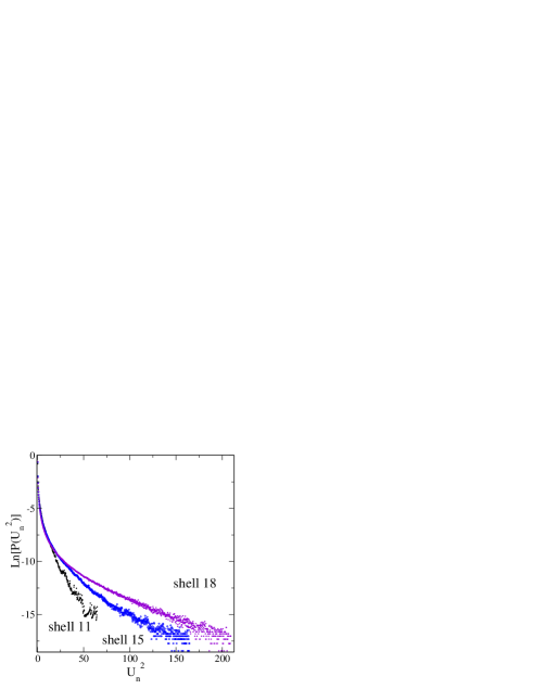
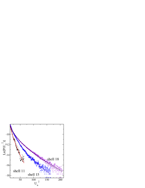
FIG. 11.: Upper panel: PDFs of the 11th, 15th and 18th shells (averaged over $10^{9}$ time steps). Lower panel: Tails of PDFs (with the cores left out) fitted by functions of the form $\ln[P_{n}(U_{n}^{2})]=a_{n}+b_{n}U_{n}$ ( continuous lines).

Our aim here is to test the predictions regarding the tails of the PDF’s. We note that PDFs that originate from data tend to have rather noisy tails. This poses difficulties in assessing the accuracy of the collapse of the tails. Therefore we opt to first fit the PDFs with some appropriate functional form and then to collapse the fit functions. As a natural fit function we choose $\ln[P_{n}(U_{n}^{2})]=a_{n}+b_{n}U_{n}^{2c_{n}}$ with three free parameters $a_{n}$, $b_{n}$ and $c_{n}$. The results of our fits showed that the parameters $c_{n}$ are close to $1/2$ for all values of $n\geq 11$. Therefore we fixed the value $c_{n}=1/2$ and optimized the values of of $a_{n}$ and $b_{n}$ to get the best fits in the tail regions. Now the fit formula reads

$$\ln[P_{n}(U_{n}^{2})]=a_{n}+b_{n}U_{n}\ .$$ (26)

The corresponding fits for the tails of the PDFs for the 11th, 15th and 18th shells are shown in Fig. 11, lower panel. The fits are excellent for $U_{n}^{2}>20$ but not surprisingly they fail for smaller values of $U_{n}^{2}$, especially for larger value of $n$.

To collapse the tails together we need to choose a reference shell $n_{\rm r}$ ; we show the results for $n_{\rm r}=11$. Replotting $\ln[P_{n}(U_{n}^{2})]-a_{n}+a_{11}$ as a function of $b_{n}^{2}U_{n}/b_{11}^{2}$ one collapses the tails of all the PDF’s on the tail of PDF for $n_{\rm r}=11$. This is shown in Fig. 12.

The theoretical predictions (18, 22) are

$$a_{n}-a_{11} = (n-11)(\alpha+\beta-z)\,\ln\lambda\,,$$ (27)

$$2\ln(b_{n}/b_{11}) = (n-11)\,\alpha\ln\lambda\ .$$ (28)

According to Eqs. (18) and the relation $y+z=1$ one computes $\alpha+\beta-z=2-3z+\beta$. We plot now the measured (by the best fits) values of $(b_{n}-b_{11})/\ln\lambda$ vs $(n-1)$. Finding best linear fits to the resulting plots we compute $\alpha=-0.25\pm 0.03$. Noticing the independently measured values of $y=0.24\pm 0.01$, $\zeta_{2}=0.72\pm 0.01$ we see that our value of $\alpha$ is in excellent agreement with Eq. (18); the latter predicts $\alpha=2y-\zeta_{2}\approx 0.24$.

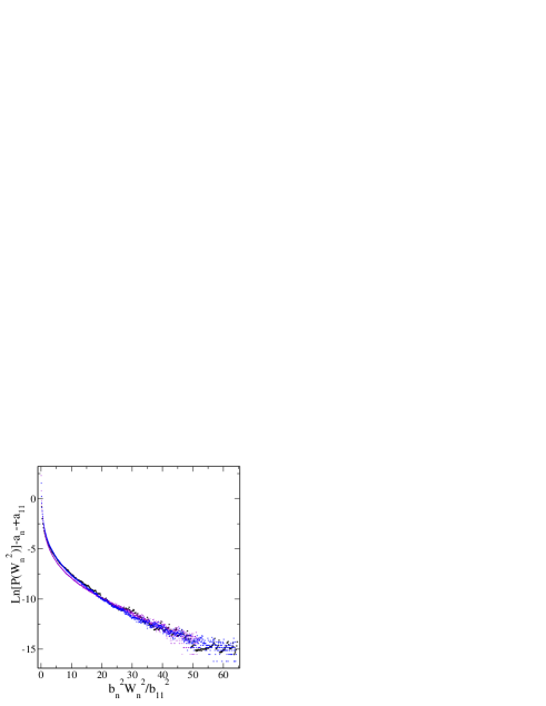
FIG. 12.: Full collapse of the PDF tails of the 11th, 15th and 18th shells. Note that in the core region the data does not collapse.

We want next to find the value of $\beta$ from the first of Eqs.(27). Unfortunately the values of $a_{n}$ are not computable with the same accuracy as those of $b_{n}$. The reason for this is that the fit formulae picks up the values of the intercepts of Eq.(26) with much worse precision than the slopes. Accordingly the plot $(a_{n}-a_{11})/\ln\lambda$ vs $(n-11)$ is much more scattered than the corresponding plot for the slopes, and we can only offer a rough estimate of the expected values of $\beta$, $0.2\leq\beta\leq 0.6$.

This rough estimate is not satisfactory, and therefore we attempt now to find a sharper result for $\beta$ using Eq.(25). In paper [8] we measured the values of $\zeta_{p}$ for $p=1,\,2,\,3,\dots 7$. We recognize that these values of $p$ are not large enough to determine the asymptotic slope of $\zeta_{p}$. Nevertheless for a semi-quantitative analysis we can use a reasonable fit formula for the $\zeta_{p}$-dependence, for example:

$$\zeta_{p}=\frac{p}{3}-\frac{\delta\,p\,(p-3)}{1+\gamma p}\ .$$ (29)

With this we find the “best” values of $\delta$ and $\gamma$ that agree with the measured values of $\zeta_{p}$: $\delta\approx 0.092$, $\gamma\approx 0.725$. With these values Eq. (29) predicts for $p\to\infty$

$$\zeta_{p}\approx 0.56+0.21\,p\ .$$ (30)

According to the prediction (25) the slope of this dependence is $y$. The value of $y$ found above from the inter-shell collapse of the separated peaks is $y=0.24\pm 0.01$, being in agreement with the value of $y$ found from the collapse of PDF tails. The value $y=0.24\pm 0.01$ differs a bit from the slope in Eq. (30). Nevertheless in light of the inaccuracy of the measured values $\zeta_{p}$ for large $p$ (originating mostly from the finite extent of the inertial interval), one cannot trust the last digits in the numbers of Eq.(30). We thus consider the agreement between the estimated values of $y$ more than acceptable.

Thus we will use the intercept in Eq. (30) to estimate $\beta$. Considering Eq. (25) the free term in (30) has to be $z-\beta$. With $z\approx 0.74$ we compute $\beta\approx 0.18$ which is at the borderline of the expected region [0.2,0.6] found above from collapsing the PDF tails. Taking then a value of $\beta\approx 0.2$ allows us to evaluate the number of peaks $N_{n}$ in $n$ shell when there were $N_{n-1}$ peaks in the previous one:

$$N_{n}/N_{n-1}=\lambda^{\beta}\approx 1.15\,,\quad\mbox{for}\ \lambda=2\,,\ \beta=0.2\ .$$ (31)

The conclusion is that peak splitting leads (for $\lambda=2$ and the chosen value of $a,b,c$) to a 15% increase of $N_{n}$ from shell to shell.

A cursory look at Fig.6 may leave the impression that this is an underestimate. After all, from one peak in shell 15 the cascade forms four or five peaks in shell 20. A rate of increase of 15% would result in a factor of 2, not 5. But we must rememeber that we talk about peaks of a given amplitude, and the peak splitting results in peaks of varying amplitudes. The counting of peaks of comparable amplitudes is more subtle, and the predicted rate of 15% increase should be interpreted in the statistical sense, taking many realizations into account.

V Self-similar solutions of the Sabra shell model

In this section we rationalize the scale-invariant form (12) on the basis of the equations of motion of the Sabra model (3). The exponent $y$ and the times $t_{n}$ which appear in Eq. ( 12) are chosen according to

$$y=1-z\,,\quad t_{n}-t_{n-1}=A\lambda^{-zn}\,,$$ (32)

with an arbitrary positive parameter $A$; (note that in [10] there was a salient choice of $A=0$). These choices are not specific for the Sabra model; in Refs. [9, 10] identical choices were taken the the Obukhov – Novikov (ON) and the Gledzer – Okhitani – Yamada (GOY) models. The fist relation follows from simple power counting, since the RHS of the equation of motion for $n$th shell is proportional to $\lambda^{n}$. Indeed, we saw that this scaling relation is in good agreement with our numerical observations. The second choice of (32) reflects the fact the time delay between the appearance of the peaks in consecutive $n$ shells falls off geometrically with $n$, and see Fig. 6 as an example. Nevertheless we want to show directly that these choices are supported by the equations of motion.

In doing so we follow Ref. [9]. Substituting (12) and (32) in (3) we find the equation of motion of the scaling function $f(\tau)$ which is valid in the inertial interval:

$$\frac{d\,f(\tau)}{d\tau} = \rm{St}(\tau)\ ,$$ (33)

$$\rm{St}(\tau) \equiv \lambda^{3z-2}f^{*}[\lambda^{z}(\tau-\tau_{0})+\tau_{0}]f[\lambda^{2z}(\tau-\tau_{0})+\tau_{0}]$$ (34)

$$+ \,\,c\lambda^{2-3z}f[\lambda^{-z}(\tau-\tau_{0})+\tau_{0}]f[\lambda^{-2z}(\tau-\tau_{0})+\tau_{0}]$$ (35)

$$- (a+c)f^{*}[\lambda^{-z}(\tau-\tau_{0})+\tau_{0}]f\,[\lambda^{z}(\tau-\tau_{0})+\tau_{0}]\ .$$ (36)

To get this equation we changed the time variable from $t$ to $\tau_{n}\equiv\lambda^{nz}(t-t_{n})$, and used the same $\tau_{n}$ in all the shells involved in (3), and finally denoted $\tau_{n}\equiv\tau$. The characteristic time $\tau_{0}$ is obtained from computing the sum of all time increments $\sum_{m=n}^{\infty}(t_{m+1}-t_{m})$, and noting that it converges to $t_{0}=\lambda^{-nz}\tau_{0}$, where

$$t_{0}=\lambda^{-nz}\tau_{0}\,,\quad\tau_{0}\equiv A/(\lambda^{z}-1)\ .$$ (37)

The meaning of $t_{0}$ is the time needed for a pulse to propagate from the $n$th shell all the way to infinitely high shells. The characteristic time $\tau_{0}$ allows one to convert all the arguments of the functions $f$ involved in (34) to a universal form $[\lambda^{\alpha}(\tau-\tau_{0})+\tau_{0}]$.

It was shown in Ref. [9] that the Eqs. (33, 34) can be considered as a nonlinear eigenvalue problem. They have trivial solutions $f(\tau)=0$, but they may have nonzero solutions for particular values of $z$ and $A$. For example, the nonzero solution $f(\tau)=\$const. requires $z=2/3$. Nevertheless the constant solution fails to fulfill the requirement that $\lim_{\tau\to\pm\infty}f(\tau)=0$. We expect that a nontrivial solution that satisfied the boundary conditions will force $z$ into the observed value which lies between 2/3 to 1. The actual calculations that demonstrate this are outside the scope of this paper. We just reiterate our numerical finding that $z\approx 0.75$ for the particular set of parameters $a$, $b$, $c$ and $\lambda$ that were employed in this study.

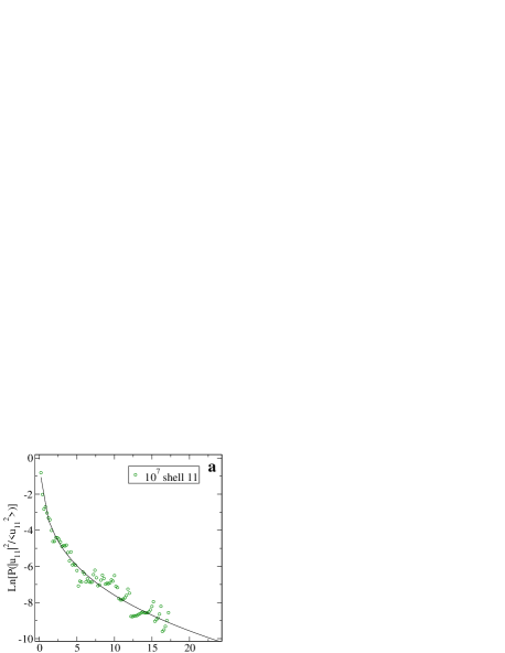
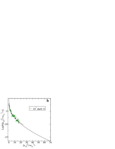
FIG. 13.: Panel a: data and analytic fit for the PDF of the 11th shell in a short time horizon of $10^{7}$ time steps. Note that here we presented all the events, including four isolated events that give rise to the upswingings strings of data points with amplitudes larger than 7. Panel b: same as in panel a together with the tail (dashed line) predicted from the tail of the 18th shell in the same short time horizon.

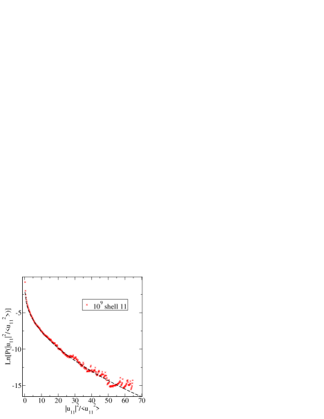
FIG. 14.: Test of the predicted PDF for the 11th shell using data from a hundred fold longer time horizon of $10^{9}$ time steps.

VI Predicting tails of PDF’s from data measured in short time horizons

In this Section we demonstrate that the analysis presented above can be used to predict the tails of the PDF’s of large scale phenomena (relatively low values of $n$) using only data measured in the short time horizon. We focus on the example shown in Fig. 2, i.e. $n=11$ with $10^{7}$ times steps.

We first fit the PDF shown in Fig. 2, using a fit formula which is inspired by Eq. (26):

$$\ln[P_{n}(u_{n}^{2})]=\tilde{a}_{n}+\tilde{b}_{n}u_{n}^{\tilde{c}_{n}}\ ,$$ (38)

and found $\tilde{a}_{11}\approx 1.34$, $\tilde{b}_{11}\approx-4.64$., $\tilde{c}_{11}\approx 0.28$. The data and the best fit are shown in Fig.13 panel a.

Next we want to continue the PDF of $n=11$ into event values that are too rare in the short time horizon. To this aim we measured, in the same time window of $10^{7}$ time steps, the tail of the PDF of the 18th shell. In doing so we use the fact that the small scale events have a much shorter turn over time, and the “short” time horizon is sufficiently long to provide a good estimate of the tail. We fitted the tail with Eq. (26) and found $a_{18}\approx-5.3$, $b_{18}\approx-0.94$. From this value and (Eq. 27) we can predict $b_{11}$. We employ the value $\alpha\approx 0.24$ which is taken from Eq.(18) with the known value of $y$ (from the intershell collapse) and of $\zeta_{2}$. The resulting prediction is $b_{11}\approx-1.72$.

Rather than attempting to also predict $a_{11}$ in Eq. (26) (knowing the inaccuracies of intercepts) we glued the tail with the predicted value of $b_{11}$ to the core PDF function (38) by finding the unique point of continuity with same first derivative. The way that the predicted tail hangs onto the PDF is shown in Fig. 13 panel b.

To test the quality of the prediction we ran now the simulation for a time horizon that is a hundred times longer (i.e $10^{9}$ time steps). Such a run can resolve the events that belong to the tail, and indeed the comparison is surprisingly good, as seen in Fig. 14.

VII Summary

The main aims of this paper are twofold: on the one hand we aimed at understanding the detailed dynamical scaling properties of the largest events in our system. On the other hand we wanted to employ these properties to predict the probability of these events even in situations in which they are very rare.

The first aim was achieved by focusing on the largest events, following their cascade down the the scales (or up the shells), and learning how to collapse them on each other by rescaling their amplitudes and their time arguments. This exercise culminated in Eq.(12) which represents the largest events $u_{n}(t)$ in terms of a “universal” function $f(\tau)$ where $\tau$ is a properly rescaled time difference from the peak time of the event. This dynamical scaling form is characterized by two exponents, a “static” one denoted $y$ and a “dynamic” one denoted $z$. We argued theoretically for a scaling relation $z+y=1$, and determined the values of the these exponents on the basis of the analysis of isolated events in short time horizons.

The second aim was accomplished by developing a scaling theory for the tails of the PDF’s in different shells. We have learned how to translate information from the tail of a PDF in a high shell to the tail of a PDF of a low shell. In doing so we made use of the fact the high shells (small length scales) have much shorter characteristic times scales. Thus even short time horizons are sufficient to accumulate reliable statistics on the tails of the PDF’s of high shells. Having a theory to translate the information to low shells in which the tails are extremely sparse (or even totally absent), we could overcome the meager statistics. We could present predicted tails that were populated only in time horizons that were a hundred fold longer than those in which the analysis was performed.

We demonstrated the existence of scaling properties of the extreme events that are in distinction from the bulk of the fluctuations that make the core of the PDF. In this sense the extreme events are outliers. We cannot, on the basis of the present work, claim that this approach has a general applicability to a large class of physical systems in which extreme events are important. We certainly made a crucial and explicit use of the scale invariance of the underlying equation of motion. This scale invariance translates here to an intimate connection between extreme events appearing on one length scale at one time to extreme events appearing on smaller length scales at later (and predictable) times (cf. Fig.6). We are pretty confident that similar ideas can (and should) be implemented to fluid turbulence; whether or not such techniques will be applicable to broader issues like geophysical phenomena or financial markets is a question that we pose to the community at large.

- [1] D. Sornette, “Complexity, catastrophe and physics”, Physics World 12 57 (1999).
- [2] A. Johansen and D. Sornette, Eur. Phys. J. B 1, 141 (1998).
- [3] E. B. Gledzer. Dokl. Akad. Nauk. SSSR, 200, 1046 (1973).
- [4] M. Yamada and K. Ohkitani. J. Phys. Soc. Jpn., 56, 4210 (1987).
- [5] M. H. Jensen, G. Paladin, and A. Vulpiani. Phys. Rev. A, 43, 798 (1991).
- [6] D. Pissarenko, L. Biferale, D. Courvoisier, U. Frisch, and M. Vergassola . Phys. Fluids A, 5, 2533 (1993).
- [7] R. Benzi, L. Biferale, and G. Parisi. Physica D, 65, 163 (1993).
- [8] V.S. L’vov, E. Podivilov, A. Pomyalov, I. Procaccia and D. Vandembrouq, Phys. Rev. E, 58, 1811 (1998).
- [9] T. Nakano. Progress of Theoretical Physics, 79, 569 (1988).
- [10] T. Dombre and Jean-Louis Gilson, On-line pub. chao-dyn/9510009 (1995).