Quantum Zeno Effect in Quantum Chaotic Systems

Abstract

We analyzed the effect of frequent measurements on the quantum systems that are chaotic in the classical limit. It is shown that the kicked rotator, a well-known example of quantum chaos, is too special to be used as a testing ground for the effects of the repeated measurements. The abrupt change of state vectors by the delta-kick singular interruptions causes a quantum anti-Zeno effect. However, in more realistic systems with interaction potentials of continuous time dependence the quantum Zeno effect prevails.

Quantum mechanical behavior of the systems that are chaotic in the classical limit, so called quantum chaos, has recently been the subject of considerable interest [1]. Now it is generally accepted that classical-like chaos is absent in quantum mechanics. We can consider dividing the whole physical problem of quantum dynamics into two qualitatively different parts: unitary time evolution of the wave function $\psi(t)$ described by Schrödinger’s equation and the collapse of the wave function caused by quantum measurements. The first part has been mostly investigated in the study of quantum chaos so far while the second part still remains controversial. The absence of classical-like chaos is agreed only in the first part. It has been stressed that, particularly by Lamb, that the clarification of quantum chaos should be based on the thorough understanding of the concept of measurements in quantum mechanics [2].

One of the most paradoxical results in the measurement problem is the quantum Zeno effect (or quantum watched pot) [3], which is the inhibition of the time evolution of a quantum system, from one eigenstate of an observable into a superposition of eigenstates, by frequently repeated measurements . It can occur when measurement are repeated so rapidly that the time between any two successive measurements is much shorter than the natural life time of the state. In his 1930 book [4], Dirac already asserted that an observation of an observable always results in one of the eigenvalues of that observable, and that two measurements of the same observable made in rapid succession would give the same results. Itano et al. experimentally found that Rabi oscillations were diminished by frequent measurements of the survival of the initial eigenstate, which was considered as the first demonstration of the quantum Zeno effect [5]. However, it is arguable whether this confirms the quantum Zeno effect completely [6, 7, 8]. Recently Kofman and Kurizki [9] found that the modification of a decay process is determined by the energy spread incurred by the measurements and by the distributions of the states to which the decaying state is coupled. They concluded, whereas the inhibitory quantum Zeno effect may be feasible in a limited class of systems, the opposite effect, accelerated decay or quantum anti-Zeno effect, appears to be much more ubiquitous.

One major modification that quantum mechanics introduces to the classical picture of the deterministic chaos is the suppression of chaotic diffusion, a phenomenon usually referred to as dynamical localization (DL). This phenomenon, first discovered by Casati et al. [10] in their investigation of the kicked rotator, can be understood as a dynamical version of Anderson localization in solids [11]. Just like the other quantum interference effects, DL is very sensitive to any incoherent perturbation. In the quantum kicked rotator, even when the corresponding classical dynamics is regular, a diffusive behavior is obtained if a measurement is performed after each kick [12]. This phenomena was interpreted as an example of the anti-Zeno effect [13]. However, in this paper we show, although the kicked rotor is a well-known example of the quantum chaos, it is too special to be used as a testing ground for the effect of the repeated measurements. The anti-Zeno effect in the kicked rotator is rather a trivial consequence of singular interruptions by the delta kicks. In more general classes of the quantum systems that are chaotic in the classical limit, the quantum Zeno effect prevails, which can be also confirmed by using the results of Kofman and Kurizki [9].

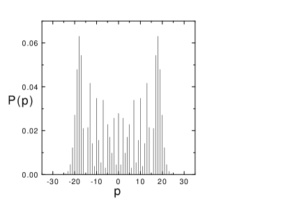
FIG. 1.: Probability distribution of the state vector in the momentum space after a single kick in the kicked rotator with the initial state $|n=0\rangle$ for $\lambda=20$ and $T=1/4$. It is noted that the survival probability, $P(1)(=|c_{0}(1)|^{2})$, is less than 3%.

Let us begin by analyzing the kicked rotator described by the following Hamiltonian

$$H=\frac{p^{2}}{2}+\lambda\cos x\sum_{k=-\infty}^{\infty}\delta(t-kT),$$ (1)

where $\lambda$ and $T$ is the kick strength and the time interval between successive delta kicks, respectively. Using the complete set of eigenstates $|n\rangle$, in which $\langle x|n\rangle=\exp(inx)/\sqrt{2\pi}$, the state just after the $(k+1)$th kick, $\psi(k+1)=\sum c_{n}(k+1)|n\rangle$, can be described by unitary transformation of the state just after the $k$th kick, $\psi(k)=\sum c_{n}(k)|n\rangle$:

$$c_{n}(k+1)=\sum_{m}U_{nm}c_{m}(k),$$ (2)

where $U_{nm}=(-i)^{n-m}J_{n-m}(\lambda/\hbar)\exp(-i\hbar m^{2}T/2)$ with $J_{n}$, the $n$th order Bessel function. Figure 1 shows the probability distribution of the state after a single kick for the initial condition $|n=0\rangle$ with $\lambda=20$ and $T=1/4$. Since during the time interval between successive kicks the momentum distribution is not changed, it is meaningless to perform the measurements more frequently than at the rate of $1/T$.

The quantum Zeno effect is represented by the relation, $P(t)\rightarrow 1$ as $\tau\rightarrow 0$, where $\tau$ and $P(t)$ represent the time interval between successive measurements and the survival probability of the initial state, respectively. Note that the Zeno effect concerns itself with the short time behavior of the quantum evolution. In the kicked rotator the Zeno effect cannot take place by the following reasons. First, since the momentum distribution does not change during the time interval between successive kicks, any measurement done during that time interval, will trivially yield an identical result. Hence, for any meaningful discussion of the Zeno effect, we should consider $\tau$ larger than the period $T$. Once we have this constraint, the fact that $P(t)$ changes abruptly even after a single kick leads us to conclude that any physically meaningful Zeno effect cannot occur in this system. The quantum localization due to the quantum interference is destroyed in the kicked rotator by the decoherence induced by the measurements. This observation is interesting but does not prove the existence of the anti-Zeno effect in a broad class of the quantum systems that are chaotic in the classical limit.

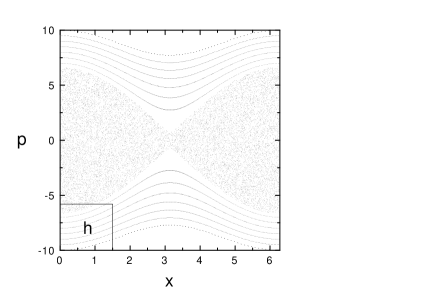
FIG. 2.: Partial Poincaré surface of section showing the phase space dynamics described by the Hamiltonian of Eq. (3) for $\lambda=10$ and $T=2\pi$. The box in the left corner illustrates the size of Planck constant $h$.

In order to analyze the effect of repeated measurements in the absence of the abrupt changes of the wave function as in the kicked rotator, we consider a new Hamiltonian with continuous time dependence:

$$H=\frac{p^{2}}{2}+\lambda\cos x\cos t.$$ (3)

It is noted that the delta kicks in Eq. (1) can be expanded as follows,

$$\sum_{k=-\infty}^{\infty}\delta(t-kT)=\frac{2}{T}\sum_{m=1}^{\infty}\cos(\frac{2\pi mt}{T})+\frac{1}{T},$$ (4)

so that Eq. (3) corresponds to the rotator driven by a single frequency mode among the infinite numbers of modes of the kicked rotator. Figure 2 shows a Poincare surface of section of Eq. (3) with $\lambda=10$, where a confined chaotic region is seen near the origin. While the diffusion of the classical kicked rotator does not stop due to the infinite number of frequency components, the classical as well as the quantum diffusion in Eq. (3) become saturated. In Fig. 3 we show that both classical and quantum evolution of $\Delta p^{2}(t)$ have the same average level except for the quantum fluctuations, so that both the quantum and classical results in Fig. 3 correspond to a delocalized regime. In our discussion it is not necessary that the quantum diffusion should be suppressed below the classical one, the so-called localized regime.

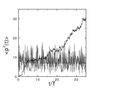
FIG. 3.: The evolution of momentum width $\Delta p^{2}(t)$ as a function of time in a unit of the period of driving field in the system described by the Hamiltonian of Eq. (3). The solid and the dotted curves represent the pure quantum evolution and the measured quantum evolution with $\tau=T/1000$, respectively. The dashed curve corresponds to the classical evolution.

Consider now the dynamics of a system subjected to measurements at time $n\tau$ ($n$ is an integer). The wave function can be expanded into a linear superposition of complete bases of an observable, say, $A$, for example

$$\psi(t)=\sum_{n}c_{n}(t)u_{n},~{}~{}~{}Au_{n}=a_{n}u_{n}\;.$$ (5)

where $c_{n}(t)=|c_{n}(t)|e^{i\phi(t)}$ with $\phi(t)$ a phase factor. A measurement of the system’s state at $t=n\tau$ projects the system onto one of the eigenstates of the measured observable $A$ with a probability $|c_{n}(t)|^{2}$. After the measurement we know the probabilities, but we lose information on the phase of the amplitudes $\phi(t)$, so that the phase after the measurement can be regarded being random. This is nothing but the simple measurement postulate, so-called von Neumann’s formulation of the wave function collapse.

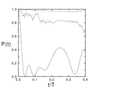
FIG. 4.: The survival probability for the pure quantum evolution (the solid curve) and the measured quantum with $\tau=T/1000$ (the dashed curve) and $\tau=T/5000$ (the dotted curve). This clearly shows quantum Zeno effect.

By using this concept we can find the quantum evolution of the system of Eq. (3) under the repeated measurements. The system is described by a unitary transformation given by Schrödinger’s equation in the momentum representation. Upon measuring the momentum we randomize the phases of all the amplitudes, which can be also expressed by a unitary transformation of a form of a diagonal matrix with random complex numbers of unity amplitude. Even though this diagonal matrix is unitary in the mathematical expression, it can be considered irreversible in time in the physical sense since the phase randomization corresponds to a stochastic process. In practice, for reducing the fluctuations induced by the phase randomization, we averaged over 100 data sets for each result. Figure 4 shows that the autocorrelation of the initial wave function (or survival probability), $|\langle\psi(0)|\psi(t)\rangle|^{2}$, without measurement (the solid curve) decreases faster than that under measurement (the dashed and the dotted curves). In addition, the shorter is the time interval of the measurement, the slower is the decay of the autocorrelation. This is exactly what the quantum Zeno effect is.

Figure 3 presents $\Delta p^{2}(t)$ for the quantum evolution both with and without measurement, where the long time behavior is totally different from the short time one. The decoherence induced by the measurements destroys quantum (and classical) localization. It should be emphasized that this delocalization (or diffusion) does not show anti-Zeno effect since Zeno effect manifests itself only in the short time limt. It is also noted that the measured quantum dynamics is not equivalent to the classical dynamics regardless of the frequency of measurements, which has been already known in several previous works [12, 14].

To gain more physical insight let us examine the present problem using the analysis tool similar to that of Ref. [9]. We write $\hat{H}=\hat{H}_{0}+\hat{V}g(t)$, so that $\hat{H}_{0}|\alpha\rangle=\hbar\omega_{\alpha}|\alpha\rangle$ and $\hat{H}_{0}|j\rangle=\hbar\omega_{j}|j\rangle$, where $|\alpha\rangle$ is an initial (decaying) state and ${|j\rangle}$’s are orthogonal to $|\alpha\rangle$. The wavefunction can be written by

$$\psi(t)=\alpha(t)e^{-i\omega_{\alpha}t}|\alpha\rangle+\sum_{j}\beta_{j}e^{-i\omega_{j}t}|j\rangle.$$ (6)

One can then obtain the following equations from Schrödinger’s equation

$$\dot{\alpha} = -\frac{i}{\hbar}\sum_{j}\langle\alpha|\hat{V}|j\rangle e^{i(\omega_{\alpha}-\omega_{j})t}g(t)\beta_{j}$$ (7)

$$\dot{\beta}_{j} = -\frac{i}{\hbar}\langle j|\hat{V}|\alpha\rangle e^{-i(\omega_{\alpha}-\omega_{j})t}g(t)\alpha.$$ (8)

Integrating (8) and inserting it into (7), we obtain the equation

$$\dot{\alpha}=-\int^{t}_{0}dt^{\prime}e^{i\omega_{\alpha}(t-t^{\prime})}\Phi(t-t^{\prime})g(t)g(t^{\prime})\alpha(t^{\prime}),$$ (9)

where

$$\Phi(t)=\hbar^{-2}\sum_{j}|\langle\alpha|\hat{V}|j\rangle|^{2}e^{-i\omega_{j}t}.$$ (10)

Since we need to obtain only the short time behavior, for which $\alpha(t)\approx\alpha(0)=1$, we can set $\alpha(t^{\prime})=1$ in the right side of Eq. (9) to obtain

$$\alpha\simeq 1-\int_{0}^{t}dxe^{i\omega_{\alpha}x}\Phi(x)M(t,x),$$ (11)

where

$$M(t,x)=\int_{x}^{t}dt^{\prime}g(t^{\prime})g(t^{\prime}-x).$$ (12)

If measurements are performed at sufficiently small interval $\tau$, we can obtain the survival probability, $P(t)$, using Eq. (11)

$$P(t=n\tau)\simeq|\alpha(\tau)|^{2n}\approx e^{-R(\tau)t},$$ (13)

where

$$R=\frac{2}{\tau}Re\int_{0}^{\infty}dte^{i\omega_{\alpha}t}\Phi(t)M(\tau,t)\theta(\tau-t).$$ (14)

The function $\theta(x)$ is 1 for $x\geq 0$ and 0 for $x<0$. Using the convolution theorem of Fourier transform, Eq. (14) can be rewritten by

$$R=2\pi\int_{0}^{\infty}d\omega G(\omega)F(\omega),$$ (15)

where

$$G(\omega)=Four\{\Phi(t)\}=\hbar^{-2}\sum|\langle\alpha|\hat{V}|j\rangle|^{2}\delta(\omega-\omega_{j})$$ (16)

and

$$F(\omega)=Four\left\{\frac{1}{\tau}M(\tau,t)e^{i\omega_{\alpha}t}\theta(\tau-t)\right\}.$$ (17)

$Four(f)$ means Fourier transform of the function $f$. While the function $G(\omega)$ in Eq. (16) is the spectral density of the states depending on the Hamiltonian, especially the coupling, $\hat{V}$, the form factor $F(\omega)$ in Eq. (17) shows the broadening of the eigenvalue $\omega_{\alpha}$ incurred by the frequent measurements. If the time independent potential is considered, simply $F_{0}(\omega)=(\tau/2\pi){\rm sinc}^{2}((\omega-\omega_{\alpha})\tau/2)$, in which the broadening rate is approximately $1/\tau$, consistent with the uncertainty principle.

In the case of a time dependent potential like the one described by Eq. (3), only $F(\omega)$ is modified from $F_{0}(\omega)$. Even though this is not just simple sinc function, the broadening of $\omega_{\alpha}$ is of the order of $1/\tau$ or larger. As the time interval of measurement, $\tau$, decreases, the broadening of $F(\omega)$ becomes larger, so that for a given $\omega$ the value of $F$ also decreases. Consequently we can roughly write $F\sim\tau$ (or monotonically increasing function of $\tau$). Since $\langle 0|\cos x|j\rangle=(\delta_{1j}+\delta_{-1j})/2$ in (3), we obtain the following simple equation

$$G(\omega)=\lambda^{2}\delta\left(\omega-\frac{1}{2}\right).$$ (18)

From these it can be easily shown that $R\sim\lambda^{2}\tau$, which means that in the limit of $\tau\rightarrow 0$, the decay rate goes to zero. This corresponds to the Zeno effect. If the delta kicks in Eq. (1) are replaced by pulses with a gaussian shape with finite time duration of interaction, which also means more harmonics are included in Eq. (3), the above discussion is still applicable, and thus we find the decay rate $R$ still proportional to $\tau$ with a different numerical constant. Therefore, for a realistic kicked rotator we reach the same conclusion, the Zeno effect.

In summary, we have investigated the effect of frequent measurements on quantum systems that are chaotic in the classical limit. In the well-known kicked rotator a meaningful Zeno effect cannot occur due to the abrupt change of state vectors by the delta kicks. For fair evaluation of measurement-induced effects a new Hamiltonian with continuous time dependence has been considered instead. In this case, it was shown that the shorter is the time interval of the measurement, the slower is the decay of the survival probability. This clearly shows the quantum Zeno effect occurs. We also examined this problem analytically and confirmed our conclusion. Even though in the case of radiative or radioactive decay quantum anti-Zeno effect prevail [9], in the usual dynamical systems including chaotic ones quantum Zeno effect is more feasible.

We thanks Hyunchul Nha, Jaewan Kim, and Hai-Woong Lee for helpful discussion. This work is supported by Creative Research Initiatives of the Korean Ministry of Science and Technology.

REFERENCES

- [1] L. E. Reichl, The Transition to Chaos in Conservative Classical Systems: Quantum Manifestations (Springer-Verlag, New York, 1992).
- [2] W. E. Lamb, Jr., in Chaotic Behavior in Quantum Systems, edited by G. Casati (Plenum, New York, 1985).
- [3] B. Misra and E. C. G. Sundarshan, J. Math. Phys. 18, 756 (1977).
- [4] P. A. M. Dirac, Principles of Quantum Mechanics (Oxford, 1930).
- [5] W. M. Itano, D. J. Heinzen, J. J. Bollinger, and , Phys. Rev. A 41, 2295 (1990).
- [6] L. E. Ballentine, Phys. Rev. A 43, 5165 (1991).
- [7] V. Frerichs and A. Schenzle, Phys. Rev. A 44, 1962 (1991).
- [8] S. Pascazio and M. Namiki, Phys. Rev. A 50, 4582 (1994).
- [9] A. G. Kofman and G. Kurizki, Nature 405, 546 (2000).
- [10] G. Casati, B. V. Chirikov, F. M. Izrailev, and J. Ford, in Stochastic Behaviors in Classical and Quantum Hamiltonian Systems, edited by G. Casati and J. Ford, Lecture Notes in Physics Vol.93 (Springer Verlag, Berlin, 1979) p. 334.
- [11] S. Fishman, D. R. Grempel, and R. E. Prange, Phys. Rev. Lett. 49, 509 (1982).
- [12] P. Facchi, S. Pascazio, and A. Scardicchio, Phys. Rev. Lett. 83, 61 (1999).
- [13] B. Kaulakys and V. Gontis, Phys. Rev. A 56, 1131 (1997).
- [14] T. Dittrich and R. Graham, Phys. Rev. A 42, 4647 (1990).