Multi-soliton energy transport in anharmonic lattices

Abstract

We demonstrate the existence of dynamically stable multihump solitary waves in polaron-type models describing interaction of envelope and lattice excitations. In comparison with the earlier theory of multihump optical solitons [see Phys. Rev. Lett. 83, 296 (1999)], our analysis reveals a novel physical mechanism for the formation of stable multihump solitary waves in nonintegrable multi-component nonlinear models.

Spatially localised solutions of multi-component nonlinear models, multi-component solitary waves, have received a great deal of attention in the last decade. In particular, recent studies in the nonlinear optics [1, 2] and Bose-Einstein condensation [3] have shown that, under certain conditions and only in multi-component systems, the formation of dynamically stable localized states and soliton complexes is possible. Unlike their single-component (or scalar) counterparts, multi-component (or vector) solitons possess complex internal structure forming a kind of “soliton molecules”, which makes them attractive, both from the fundamental and applied point of view, as composite and reconfigurable carriers for a transport of spatially localized energy.

Recent discovery of stable multi-component spatial solitons in optics [1, 2] shed a light on the general physical mechanisms of the formation and stability of multi-component localised states. Such states are often called multihump solitons due to multiple maxima displayed in their intensity profile. Usually, multihump solitary waves appear via bifurcations of scalar solitons when a primary soliton plays a role of an effective waveguide (“potential well”) that traps higher-order guided modes excited in a complimentary field [2]. On the other hand, the multihump solitons can be formed as multi-soliton bound states, when two or more different vector solitons are “glued” together due to balanced interaction between the soliton constituents [4].

Soliton bifurcations and binding enable the existence of multi-component localized states in many nonlinear models; these include bound states of dark solitons [4] and incoherent solitons [5] in optics, and multihump plasma waves [6]. Importantly, multihump solitary waves are also found in higher dimensions [6, 7].

The experimental and theoretical results on optical solitons [1, 2] challenge the conventional view on multi-component solitary waves in other fields of nonlinear physics. The main question we wish to address here is: Can stable multihump solitons exist in other important models of nonlinear physics? This is a crucial issue because, so far, the stable multihump solitons have been positively identified only in the nonlinear optical model of Refs. [1, 2] that is known to possess additional symmetries, which might be the reason for their unique stability.

In this Letter, we demonstrate the existence of dynamically stable multihump solitary states in a completely different (in both the physics and properties) but even more general model that describes the interaction of envelope and lattice excitations, a generalisation of the well-known polaron model. We reveal a novel physical mechanism for the formation of stable multihump solitary waves in nonintegrable multi-component nonlinear models.

Model. Let us consider the continuous model of the energy (or excess electron) transport in an anharmonic molecular chain [8], described by the system of coupled nonlinear Schrödinger (NLS) and Boussinesq equations:

$$i\frac{\partial\psi}{\partial t} + \frac{\partial^{2}\psi}{\partial x^{2}}+2w\psi=0\;,$$ (1)

$$m\frac{\partial^{2}w}{\partial t^{2}} = \frac{\partial^{2}w}{\partial x^{2}}+\mu\frac{\partial^{4}w}{\partial x^{4}}+\alpha\frac{\partial(w^{2})}{\partial x^{2}}-\frac{\partial(|\psi|^{2})}{\partial x^{2}}\;,$$ (2)

where $t$ and $x$ are the normalised time and spatial coordinate, correspondingly, $\psi(x,t)$ is the excitation wave function, and $w(x,t)$ is the chain strain. The system is characterized by three dimensionless parameters: the particle mass $m$, the anharmonicity of the chain $\alpha$, and the dispersion coefficient $\mu$.

Equation (1) appears in a number of other physical contexts including, for example, the interaction of nonlinear electron-plasma and ion-acoustic waves [9], coupled Langmuir and ion-acoustic plasma waves [10], interaction of optical and acoustic modes in diatomic lattices [11], particle theory models [12], etc.

System (1) is known to be integrable for $\alpha\mu=6$ [13]. In this case, it possesses two types of single-soliton solutions: scalar ($\psi=0$) supersonic Boussinesq (${\mathcal{B}}$q) solitons and vector Davydov-Scott (DS) solitons [8] which can be both subsonic and supersonic. Because of the complete integrability for $\alpha\mu=6$, these solitons do not interact with each other. For $\alpha\mu\neq 6$, the situation changes dramatically, and it has been recently shown [14, 15] for the nearly-integrable case ($\alpha\mu\approx 6$) that ${\mathcal{B}}$q and DS solitons can form a bound state for $\alpha\mu>6$. From the other hand, it is also known that in a weakly anharmonic lattice two subsonic DS solitons can form a bisoliton [16]. However, it remains a mystery what happens when the system (1) is far from its integrable limit and, especially, when the solitons are supersonic. In this Letter we examine the model (1) numerically for arbitrary values of $\alpha\mu$ and, employing the concept of soliton bifurcations, demonstrate the origin and exceptional robustness of multihump supersonic stationary solitary waves.

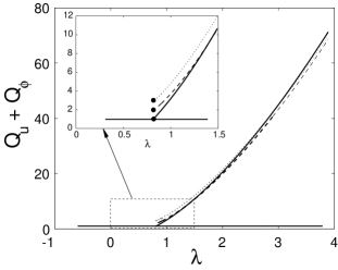
FIG. 1.: Bifurcation diagram of the system (4) for $g=7$. Inset - close-up of the bifurcation point. Horizontal line - $u$-solitons, solid - single-hump $|0,0\rangle$ solitons, dashed - two-hump solitons, dotted - three-hump solitons.

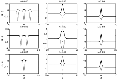
FIG. 2.: Profiles of single-hump (bottom row), two-hump (middle row), and three-hump (top row) solitons with increasing (from left to right) values of $\lambda$.

Bifurcation analysis. The stationary solutions of Eq. (1) can be found in the form of the traveling waves

$$\psi(x,t)=\frac{c}{4\sqrt{\mu}}e^{ivx/2-i\Omega t}\phi(z)\;,\quad w(x,t)=\frac{c}{4\mu}u(z)\;,$$ (3)

where $z=\sqrt{c/4\mu}(x-vt)$, and the constant $c=(mv^{2}-1)$ is positive for a supersonic velocity, $v>1/\sqrt{m}$. Substituting Eq. (3) into Eq. (1), we derive a system of coupled ordinary differential equations

$$\phi_{zz}-\lambda\phi+2u\phi=0\;,$$ (4)

$$u_{zz}-4u+gu^{2}-\phi^{2}=0\;,$$ (5)

where $g=\alpha\mu$ is an effective anharmonicity parameter, and $\lambda=\mu(v^{2}-4\Omega)/c$ is a characteristic eigenvalue of the stationary localized solutions.

Equation (4) has two types of one-soliton solutions: a one-component ${\mathcal{B}}$q soliton

$$\phi_{0}(z)=0\;,\qquad u_{0}(z)=(6/g)\,\mbox{sech}^{2}(z)\;,$$ (6)

which exists for arbitrary values of $g$, and a two-component DS soliton

$$\phi_{1}=2\sqrt{\lambda(\lambda-1)}\,\mbox{sech}(\sqrt{\lambda}z)\;,\quad u_{1}=\lambda\,\mbox{sech}^{2}(\sqrt{\lambda}z)\;,$$ (7)

which exists only in the integrable case $g=6$.

To understand what happens for $g\neq 6$, we consider the limit $\phi/u\sim\varepsilon\ll 1$ and apply a multi-scale asymptotic analysis. In the zeroth order in $\varepsilon$, $\phi=0$ and Eq. (4) reduces to a nonlinear equation for the component $u(z)$ only, with the supersonic ${\mathcal{B}}$q soliton solution (6). In the first order in $\varepsilon$, we obtain a linear eigenvalue problem for $\phi(z)$ characterized by the effective potential $u=u_{0}(z)$. For a given value of $g$, the spectrum of the eigenvalue problem consists of $N+1$ discrete eigenvalues $\lambda_{n}=\left(N-n\right)^{2}$, where $n=0,\;1,\;...\;N,$ and $N$ is the integer part of $(1/2)[\sqrt{1+(48/g)}-1]$. Each cut-off value $\lambda_{n}$ corresponds to a bifurcation point of the node-less scalar soliton $u_{0}$ where a two-component solution with a nonzero component $\phi$ emerges. The latter has $n$ nodes and, near the bifurcation point, can be treated as a fundamental (or higher-order) bound mode of an effective potential created by the soliton $u_{0}(z)$. The emerging vector soliton can therefore be characterised by a “state vector” $|0,n\rangle$, according to the number of nodes in the corresponding components.

It is easy to see that for $g>6$ only bifurcations of the $|0,0\rangle$ state, which corresponds to the DS soliton (7), are possible. First bifurcation of the $|0,1\rangle$ state occurs for the completely integrable case $g=6$ at $\lambda_{1}=0$. In this case, the bifurcation pattern is identical to that of the completely integrable Manakov limit of two coupled NLS equations [17], namely, the $|0,0\rangle$ state appears at $\lambda_{0}=1$, and the $|0,1\rangle$ state appears at $\lambda_{1}=0$.

Weaker anharmonicity (smaller $g$) means larger number of possible bound states supported by the effective potential $u(z)$, and thus the increasing number of bifurcations. Indeed, the depth of the effective trapping potential is inversely proportional to $g$. The $|0,0\rangle$ state always exists, even for a shallow potential $u(z)$.

We now consider in detail the formation of multihump solitons in the cases of weak (subcritical, $g<6$) and strong (supercritical, $g>6$) anharmonicity, respectively.

Supercritical regime. In the absence of bifurcating higher-order solutions, the multihump solitons are formed only via binding of the $|0,0\rangle$ vector solitons. The physics of this mechanism is simple. The interaction forces between closely separated fundamental solitons are different for both the $\phi$ and the $u$ components. Namely, while two in-phase $u$-solitons attract, the two in-phase $\phi$-solitons repel. This allows for the existence of multihump nodeless modes of the field $\phi$ trapped in the multi-well potential $u$. Each of such multihump solitons can be considered as a bound state of several $|0,0\rangle$ DS solitons, with in-phase humps in both components.

It is convenient to represent the solution families as branches on the bifurcation diagram $Q$ vs. $\lambda$, where $Q\equiv Q_{u}+Q_{\phi}\equiv\int u^{2}dz+\int\phi^{2}dz$ is the total soliton power. Typical bifurcation diagram for a supercritical case ($g=7$) is shown in Fig. 1. Solid line represents the bifurcating solution $|0,0\rangle$, and it can be seen on the close-up of the bifurcation region, that the branches representing two- and three-hump solutions start off at the same point $\lambda=\lambda_{0}$ but with the energies approximately equal to that of two or three $u$-solitons. Examples of such multihump solitons are shown in Fig. 2, and it is clear that this novel type of soliton bifurcations occurs from a countable set of infinitely separated single solitons. With increasing $\lambda$, separation between the humps decreases until all solitons of this type become single-humped (Fig. 2, right column).

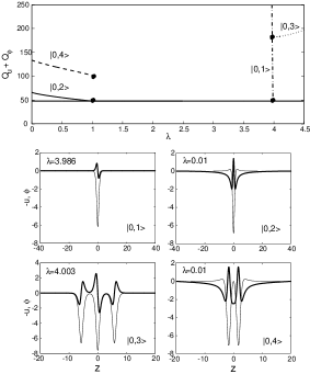
FIG. 3.: Bifurcation diagram of the system (4) for $g=1$. Shown are branches of the fundamental $u-$soliton (horizontal), $|0,1\rangle$ (dot-dashed), $|0,3\rangle$ (dotted), $|0,2\rangle$ (solid), and $|0,4\rangle$ (dashed) solitons. Below: profiles of $|0,1\rangle$ and $|0,2\rangle$ solitons (top row) and some examples of their bound states, $|0,3\rangle$=$|0,1\rangle$+$|0,1\rangle$+$|0,1\rangle$ and $|0,4\rangle$=$|0,2\rangle$+$|0,2\rangle$ (bottom row).

Subcritical regime. In this case, bifurcations of the $u$-state do not lead to multihump solitons. That is, in sharp contrast to the coupled NLS equations describing vector solitons in nonlinear optics, none of the higher-order states $|0,n\rangle$ become multihumped in the system under consideration. Although the function $\phi$ does have multiple maxima in its intensity profile, because of the non-self-consistent source for the $u$-component, it does not cause significant distortions in the shape of the effective potential, $u(z)$, and the total intensity $I(z)=u^{2}+\phi^{2}$ remains single-humped. Typical bifurcation diagram for the case $g=1$ is presented in Fig. 3. In this case $N=2$, and only bifurcations of the $|0,1\rangle$ (dot-dashed line) and $|0,2\rangle$ (solid line) solitons are shown. Corresponding modal profiles of the bifurcating solitons are presented in Fig. 3 (top row).

Similar to the supercritical regime, the multihump solitons can exist only as bound states of the bifurcating $|0,1\rangle$ or $|0,2\rangle$ solitons. They appear at the bifurcation points $\lambda_{n}$, and they have energies equal to a number of lower-order solitons “glued” together by the low-amplitude components. The number of nodes that the $\phi$-component has in the composite soliton depends on the number of $|0,n\rangle$ solitons forming that bound state. Typical examples of such solutions are presented in Fig. 3 (bottom row).

From this analysis, we can conclude that, in this model, the multihump solitons appear as bound states of $|0,0\rangle$ solitons for any value of anharmonicity parameter $g$. In addition, multihump solitons of more sophisticated modal structure are also possible.

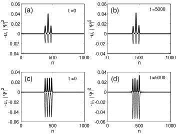
FIG. 4.: (a,b) Stable dynamics of a three-hump soliton for $g=7$ and $\lambda=0.824$. The family of these solitons is shown in Fig. 1 (dotted line), and the corresponding profiles are presented in Fig. 2 (top row). (c,d) Stable dynamics of a four-hump soliton for $g=3.005$ and $\lambda=2.9$.

Dynamical stability. The second equation of the system (1) is the so-called “ill-posed” (or “bad”) ${\mathcal{B}}$q equation [18]. It possesses an intrinsic linear instability and therefore its reliable numerical solution for non-zero $\mu$ is unfeasible. This linear instability is not inherent in the original physical model, and it can be traced to neglecting higher-order spatial derivatives in Eq. (1). In the case of the energy transport in anharmonic molecular chains, Eq. (1) with $\mu=1/12$ originates from the following system of discrete equations [14, 15]

$$i\frac{d}{dt}\Psi_{n} = -\Delta_{2}(\Psi_{n})-(W_{n}+W_{n-1})\Psi_{n}\;,$$ (8)

$$m\frac{d^{2}}{dt^{2}}W_{n} = \Delta_{2}(W_{n})+\alpha\Delta_{2}(W^{2}_{n})$$ (9)

$$+ \frac{1}{2}(|\Psi_{n+1}|^{2}+|\Psi_{n}|^{2}-|\Psi_{n-1}|^{2}-|\Psi_{n+2}|^{2})\;,$$ (10)

where $\Delta_{2}(X_{n})\equiv X_{n+1}+X_{n-1}-2X_{n}$. Discrete functions $\Psi_{n}$ and $W_{n}$ define, in the continuous limit, the excitation wave function, $\psi(x,t)$, and the strain function of the lattice, $w(x,t)$.

Therefore, it would be justified to study the dynamics of the stationary solutions of Eqs. (4) numerically by employing the original discrete dynamical system (8). Besides, the argument can be reversed, and such a discrete system can be treated as a regularised numerical discretisation scheme for a general system of coupled NLS and ill-posed ${\mathcal{B}}$q equations.

We investigate the dynamical stability of the multihump solitons for two distinct cases of a subcritical and supercritical anharmonicity discussed above. The condition of a unit norm for the envelope function $\Psi_{n}$ ($\sum_{n}|\Psi_{n}|^{2}=1$) is satisfied in all cases, and $v$ is chosen close to the sound velocity ($c=0.0244$) to allow for a smooth discretisation.

In the supercritical regime ($g>6$), where multihump solitary waves can be formed through binding of several $|0,0\rangle$ states together, our numerical simulations indicate that such solitons are stable as long as the separation between the humps is sufficiently large. This property is just opposite to that observed for multihump optical solitary waves [2]. An example of the stable dynamics of a three-hump soliton for $g=7$ is shown in Figs. 4(a,b). All solitons of the DS type, i.e. $|0,0\rangle$ soliton states, presented in Fig. 1 (by solid line) and Fig. 2 (bottom row), exhibit similar stable dynamics.

It is important that the same mechanism of the creation of multihump solitons applies to the subcritical regime. This means that the dynamically stable multi-soliton bound states described above exist also for $g<6$. As an example, propagation of a four-hump soliton at $g=3.005$ is demonstrated in Figs. 4(c,d). After initial adjusting of the soliton amplitudes (due to the discretisation), only small amplitude breathing occurs [see Fig. 4(d)], otherwise the soliton dynamics is stable. In contrast, all bifurcating higher-order solitons are dynamically unstable.

Our results on the robustness and stability of multi-soliton states call for a systematic revision of our understanding of the role of nonlinear localized modes in a number of physical phenomena related to the nonlinear transport in macromolecules [8] and even artificial nanoscale structures [19], where the coupling of two (or more) degrees of freedom occurs. How the soliton binding and existence of multi-soliton states modifies the nonlinear kinetics, nonequilibrium thermodynamics [20], and other properties of the system? These questions remain to be answered.

In conclusion, we have found robust two-component solitary waves in a polaron-type model of the energy transport in anharmonic lattices. We have revealed a novel physical mechanism for the formation of multihump solitons in a discrete anharmonic lattice and demonstrated their dynamical stability. Along with the recent studies on multihump optical solitons [1, 2], these results call for re-examination of the role of multi-component solitary waves in other fields of nonlinear physics.

We thank A. V. Zolotaryuk and L. Cruzeiro-Hansson for helpful discussions. S. M. acknowledges support from the Australian Research Council. The work of E. O. and Yu. K. is supported by the Performance and Planning Fund of The Australian National University.

REFERENCES

- [1] M. Mitchell, M. Segev, and D.N. Christodoulides, Phys. Rev. Lett. 80, 4657 (1998).
- [2] E.A. Ostrovskaya, Yu.S. Kivshar, D. Skryabin, and W. Firth, Phys. Rev. Lett. 83, 296 (1999).
- [3] See, e.g., M. R. Matthews, B. P. Anderson, P. C. Haljan, D. C. Hall, C. E. Wieman, and E. A. Cornell, Phys. Rev. Lett. 83, 2498 (1999); Victor M. Perez-Garcia, Juan J. Garcia-Ripoll, Phys. Rev. A 62, 033601 (2000).
- [4] E. A. Ostrovskaya, Yu. S. Kivshar, Z. Chen, and M. Segev, Opt. Lett. 24, 327 (1999); Z. Chen, M. Acks, E. A. Ostrovskaya, and Yu. S. Kivshar, Opt. Lett. 25, 417 (2000).
- [5] M. Mitchell, M. Segev, T.H. Coskun, and D.N. Christodoulides, Phys. Rev. Lett. 79, 4990 (1997); D.N. Christodoulides, T.H. Coskun, M. Mitchell, and M. Segev, Phys. Rev. Lett. 80, 2310 (1998).
- [6] I. A. Kol’chugina, V. A. Mironov, and A. M. Sergeev, JETP Lett. 31, 304 (1980); V. A. Mironov, A. M. Sergeev, and E. M. Sher, Sov. Phys. Dokl. 26, 861, (1981).
- [7] Z. Musslimani, M. Segev, D.N. Christodoulides, and M. Soljačić, Phys. Rev. Lett. 84, 1164 (2000).
- [8] A. S. Davydov, Solitons in Molecular Systems (Reidel, Dordrecht, 1987); A. C. Scott, Phys. Rep. 217, 1 (1992).
- [9] K. Nishikawa, et al., Phys. Rev. Lett. 33, 148 (1974).
- [10] V. G. Makhankov, Phys. Lett. A 50, 42 (1974).
- [11] N. Yajima and J. Satsuma, J. Prog. Theor. Phys. 62, 370 (1979).
- [12] G. Brown and A. D. Jackson, The Nucleon Nucleon Interactions (North-Holland, Amsterdam, 1976).
- [13] I. M. Krichever, Funct. Anal. Appl. 20, 203 (1986).
- [14] Yu. B. Gaididei, P. L. Christiansen, and S. F. Mingaleev, Physica Scripta 51, 289 (1995); S. F. Mingaleev et al., J. Biol. Phys. 25, 41 (1999).
- [15] A. V. Zolotaryuk, K. H. Spatschek, and A. V. Savin, Europhys. Lett. 31, 531 (1995); Phys. Rev. B 54, 266 (1996).
- [16] L. S. Brizhik and A. S. Davydov, Sov. J. Low Temp. Phys. 10, 358 (1984); L. S. Brizhik and A. A. Eremko, J. Biol. Phys. 24, 233 (1999).
- [17] S. V. Manakov, Sov. Phys. JETP 38, 248 (1974).
- [18] P. Rosenau, Phys. Lett. A 118, 222 (1986).
- [19] See, e.g., A. A. Farajian, K. Esfarjani, and Y. Kawazoe, Phys. Rev. Lett. 82, 5084 (1999).
- [20] L. Cruzeiro-Hansson and S. Takeno, Phys. Rev. E 56, 894 (1997).