Low-dimensional dynamical system model for observed coherent structures in ocean satellite data

Abstract

The dynamics of coherent structures present in real-world environmental data is analyzed. The method developed in this Paper combines the power of the Proper Orthogonal Decomposition (POD) technique to identify these coherent structures in experimental data sets, and its optimality in providing Galerkin basis for projecting and reducing complex dynamical models. The POD basis used is the one obtained from the experimental data. We apply the procedure to analyze coherent structures in an oceanic setting, the ones arising from instabilities of the Algerian current, in the western Mediterranean Sea. Data are from satellite altimetry providing Sea Surface Height, and the model is a two-layer quasigeostrophic system. A four-dimensional dynamical system is obtained that correctly describe the observed coherent structures (moving eddies). Finally, a bifurcation analysis is performed on the reduced model.

I Introduction

In the last decades the study of turbulent or extended chaotic systems has enjoyed important advances. Two of them are, first, the recognition of the existence and high relevance of coherent structures (defined as strongly persistent spatiotemporal structures in the dynamical evolution of the system) in weakly and even strongly chaotic systems, and, second, the borrowing of mathematical methods coming from the studies of nonlinear dynamical systems (see [1] and references therein).

In both subjects, the introduction of the statistical technique known as the Proper Orthogonal Decomposition (POD, also known under a variety of other names, such as Karhunen-Loève decomposition, method of Empirical Orthogonal Eigenfunctions, etc.) has played an important rôle. It was introduced in the context of turbulence by Lumley [2] and has revealed itself as an efficient technique for finding, describing and modeling coherent structures in turbulent fluids or extended chaotic systems. The purpose of POD is to separate a given data set into orthogonal spatial and temporal modes which most efficiently absorb the variability of the data set.

The power of POD has been implemented following two different paths [1]: On the one hand the POD is used as a standard technique to extract coherent structures from empirical data sets [3, 4]. Contrasting to Fourier Decomposition, the eigenfunctions obtained from the POD may display spatial localization, and thus provide a more efficient way to represent coherent structures. The use of empirical information can be pushed further and methodologies from dynamical systems theory and other fields have been used in the POD framework, to provide useful algorithms for control [5] and prediction [6, 7]. On the other hand, the POD eigenfunctions provide a set of basis functions which is optimum (at least in a well defined linear sense) for obtaining low-dimensional ordinary differential equation (ODE) approximations starting from models based on partial differential equations (PDEs). The approximation is performed by obtaining long runs of the PDEs, performing the POD onto this synthetic data set, and using the Galerkin method to project the PDE model into the so obtained POD eigenfunctions [8, 9, 10, 11, 12].

These two potentialities, i.e. the ability to extract empirical information from experimental data, and the efficiency in building low-dimensional projections from models, are not frequently used together in the literature. A remarkable exception is the use of empirical eigenfunctions obtained from the POD of experimental data from a turbulent boundary layer to build a low-dimensional approximation to the Navier-Stokes equations [13, 14]. We believe that, in some circumstances, the projection of theoretical models into experimentally obtained empirical functions could improve both the model and the data. This will occur in situations such as in the modeling of natural phenomena (ocean or atmospheric dynamics, for example) where even very complex models may be not accurate enough, and data are unvoidably noisy and difficult to calibrate. Projecting the model onto the experimental eigenfunctions will force it to stay into the ‘right’ subspace, providing a kind of data assimilation [15] that may compensate the loss of details inherent to low-dimensional projections. On the other hand, the truncation involved in the POD method implies a kind of filtering providing noise reduction to the data set.

Our aim in this Paper is to explore the synergy between experimental observation and low-dimensional reduction via POD, in the complex setting of environmental fluid dynamics. In particular, a model for coherent structures arising from instabilities of the Algerian current in the Mediterranean Sea will be set up and analyzed.

In the ocean dynamics context, the kind of spatiotemporal data sets we need for our purposes can only be obtained from satellite observations. The recent availability of satellite data of the sea surface is allowing a deeper understanding of the Ocean. Satellites continuously measure sea temperature, sea level, chlorophyll concentration, etc., which increase our knowledge of ocean currents, mean sea level changes, tides, or plankton dynamics, to name a few. In particular, in the last decade the ERS and the TOPEX/POSEIDON (T/P) satellite missions have provided the scientific community with high-accuracy altimetry data, which determines the sea surface level, this is, the height of the sea surface over a reference level on Earth. Among other relevant scientific applications, these type of data are specially useful for a better understanding of the dynamics of mesoscale phenomena in the Ocean. Mesoscale refers to typical spatial scales of $30$ to $300$ kilometers and time scales of less than one year, and it is associated with movements of oceanic currents and short-time flow variations, and also with the formation and propagation of ocean eddies. These eddies are generated by interactions with the oceanic topography and/or mean flow instabilities and their importance is enormous: for example they play a fundamental role in the heat transport from low to high latitudes.

Some details of the results we present here are determined by the peculiarities of the data set we are going to use. In particular we mainly focus in the motion of a vortex which is present in the data, but is only described by subdominant eigenfunctions in the POD results. This lead us to a model for this coherent structure, but we do not try to model the full dynamics of whole data set. We expect however that our general methodology will be useful in other problems in which real-world noisy observations and complex but imperfect PDE models are available. Generalizations of the POD method which take into account in a more consistent way dynamic constraints have been developed [16, 17, 18] and even applied to geophysical contexts [16, 19, 20]. We will use however, and just for simplicity, the standard formulation of the POD technique.

The Paper is organized as follows: in the next section, we describe the data set. In section III, these data are analyzed with the Proper Orthogonal Decomposition (POD). The study of the most relevant of the eigenfunctions allows the identification of a coherent structure, that is, a moving vortex or eddy. Then, in the following section, the associated temporal modes of the POD eigenfunctions defining the eddy are projected over a hydrodynamic model which, finally, provides a deterministic dynamical system depending on the parameters of the model. In section V, the reconstruction of the moving vortex from the dynamical system model is performed. Next, in section VI the bifurcation analysis of the dynamical system is shown. Section VII concludes this work.

II Satellite altimetry data

We analyze altimetry data from the T/P and ERS-1 satellite missions [21]. Altimetry data of the Ocean provide the Sea Surface Height (SSH) over a reference substrate. The data obtained in both missions have been merged (to obtain a better spatiotemporal resolution) on a common time period, from October 1992 to December 1993 and, finally, $44$ maps taken every $10$ days on a $0.2^{o}$ regular grid are obtained for the Western Mediterranean Sea [22]. We restrict our analysis to the area known as the Algerian Current, localized between $0-15^{o}E$ and $35-40^{o}N$, where a strong mesoscale activity is observed [24]. A mean flow moving eastwards and parallel to the coast of Algeria is the main feature in this area. It undergoes instabilities that shed vortices into the western Mediterranean basin, greatly influencing the physical and biological processes in this area of the Sea [23]. In Figure 1 a) we show in a small box of an image of the Mediterranean Sea, the area under study. Figure 1 b) shows one of the $44$ maps that we are going to analyse.

The SSH fields allow the identification of coherent structures (structures approximately maintained in the flow over long time periods) in geophysical flows. In particular, areas of higher altimetric values may correspond to anticyclonic (clock-wise) vortices and lower ones may indicate the existence of cyclonic (anticlock-wise) vortices. Actually, the data we have used are referred to a mean level, i.e, we analyze Sea Level Anomalies (SLA) where the reference height is the temporal mean of the data. This may give rise to some minor problems because to obtaining the SSH data (the one we are going to need in our modeling approach) is not as simple as adding the mean sea level. This is because of the different resolution in the data and will be explained in detail in section IV.

III POD analysis of the satellite data

As it has already been mentioned, the POD technique is generally used to analyze experimental or numerical data with the view in extracting their dominant features, which will typically be patterns in space and time. On output, it provides a set of orthogonal functions which are the eigenfunctions of the covariance matrix of the data. Generally, this set is ordered in decreasing size of the corresponding eigenvalue, the larger the eigenvalue meaning the larger percentage of the data variance is contained in the dynamics of corresponding eigenfunction. Thus, if $u(x,y,t)$ is our data field ($(x,y)\in A\subset R^{2}$ is the spatial point and $t$ is time) to which the temporal average has been subtracted, the POD basis $\{\phi_{i}(x,y),i=1,...,\infty\}$ is obtained after solving

$$\int_{A}<u(x,y,t)u(x^{\prime},y^{\prime},t)>\phi_{i}(x^{\prime},y^{\prime})dx^{\prime}dy^{\prime}=\lambda_{i}\phi_{i}(x,y),$$ (1)

being $<\cdot>=\frac{1}{T}\int_{0}^{T}\cdot$ $dt$, i.e., the time average, and $\lambda_{i}$ the corresponding eigenvalues, which are ordered in decreasing size $\lambda_{1}\geq\lambda_{2}\geq...\geq 0$. Therefore, we have the modal decomposition

$$u(x,y,t)=\sum_{i=1}^{\infty}a_{i}(t)\phi_{i}(x,y),$$ (2)

where the $a_{i}(t)$ are the so-called temporal modes. In addition, the following orthogonality conditions are fulfilled

$$\int_{A}\phi_{k}(x,y)\phi_{l}(x,y)dxdy=\delta_{kl},$$ (3)

$$\left<a_{k}(t)a_{l}(t)\right>=\frac{1}{T}\int_{0}^{T}a_{k}(t)a_{l}(t)dt=\lambda_{k}\delta_{kl},$$ (4)

where $\delta_{kl}$ is the Kronecker delta.

The optimality of the POD basis functions means that [1], among all linear decompositions with respect to an arbitrary basis $\{\Phi_{i}(x,y)\}$, for a truncation or order $N$, i.e., $u^{N}(x,y,t)=\sum_{i=1}^{N}a_{i}(t)\Phi_{i}(x,y)$, with $a_{i}(t)=\int_{A}u(x,y,t)\Phi_{i}(x,y)$, the minimum error, defining the error as $\epsilon=\left<\int_{A}(u-u^{N})^{2}dxdy\right>$, is obtained when $\{\Phi_{i}(x,y)\}$is the POD basis $\{\phi_{i}(x,y)\}$.

We now apply the POD analysis to the altimetry satellite data. The results of this are outlined in the following. Fig. 2 shows (in linear-log scale) the fraction of variance ${\lambda_{i}}/({\sum_{n=1}^{N}\lambda_{n}})$, given by each eigenvalue. It is clearly seen that most of the variance is captured by the first and second eigenvalues. In Fig. 3 we show the temporal mode associated to the first two eigenvalues, and the power spectrum of the four dominant ones is plotted in Fig. 4. The annual seasonal periodicity is clearly observed in the two dominant modes. This and more detailed observations in terms of a complex version of the POD on the same data set [24] allow us to interpret the dynamics given by these dominant eigenfuntions as the seasonal response of the Ocean (heating in summer and cooling in winter) along the annual cycle.

Therefore, to get a deeper insight into the data (and in particular in the mesoscale phenomena), we have to study other eigenfunctions than the first two. In Fig. 5 we show again the fraction of variance of the eigenvalues (linear-log plot) but in this case we have removed the first two eigenvalues. We observe that eigenvalues $3^{rd}$ and $4^{th}$ are equivalent under the error bar (for calculating error bars in POD eigenvalues see [25]). In this case, a linear superposition of them can represent a moving coherent structure [3]. In Fig. 6 we show the temporal modes associated with eigenvalues $3^{rd}$ and $4^{th}$. This Figure, and the corresponding power spectra in Fig. 4 suggest a weak semiannual periodicity for both modes.

Visualization of the time evolution of the data filtered to keep just the eigenfuntions $3^{rd}$ and $4^{th}$, i.e., $u_{34}(x,y,t)=a_{3}(t)\phi_{3}(x,y)+a_{4}(t)\phi_{4}(x,y)$, suggest a vortex moving northward and eastwards from the Algerian coast, in agreement with the results of [24]. The approximate periodicity of the associated temporal modes indicates that new vortices are shed from the coast roughly every six months. Describing the dynamics of this coherent structure found in the flow will be our goal in the remaining of the Paper.

IV Model and low-dimensional dynamical system

The classical way of using POD to obtain a low-dimensional dynamical system approximation, which takes into account the most relevant features of the physical system, consists in truncating the expansion (2) to a particular order [1, 8, 9, 10, 11, 12, 13, 14]. This order is generally chosen to contain most of the percentage of the variance of the data. Then, the equations governing the dynamics of the system (PDEs from which the data may have been generated numerically) are projected over this particular Galerkin basis and a system of ODEs for the temporal modes $a_{i}(t)$ can be obtained. Our approach is somewhat different, first of all, our data are from satellite observations and we need a specific mathematical model to describe approximately our data, and second, our interest focuses in the dynamics associated with the eigenfuntions $3^{rd}$ and $4^{th}$ which seem to contain the evolution of the moving mesoscale vortex, and not the more dominant eigenfunctions $1^{st}$ and $2^{nd}$.

Proceeding with the modeling step, and supported by marine experimental campaigns [24, 26], we assume that the strong mesoscale activity in the Algerian current is mainly due to baroclinic instability phenomena. This name refers to the instabilities grown from the available potential energy associated with horizontal gradients of density [28]. Therefore, we choose a two-layer quasigeostrophic model as our basic flow description since this is the minimal model accounting for these type of instabilities. Layered quasigeostrophic models are widely used in oceanographical modeling and their main assumption is that the Ocean behaves as having different layers where density is constant and, in all the different layers, geostrophic balance is maintained (i.e. Coriolis and pressure forces nearly equilibrate via a quasibidimensional flow). Actually, the spatial scales of the chosen region, and its strong topographic features, lead however to important deviations from quasigeostrophy. Thus, the postulated model should be considered at most as a crude approximation to the real dynamics. It is one of the objectives of this Paper to show that the the empirical information contained in the satellite data is incorporated into the model during the projection procedure, so that the final low-dimensional model gives a reasonable description of the dynamics.

In the framework of multilayer quasigeostrophic models, every fluid layer $i$ of density $\rho_{i}$ and thickness $h_{i}$ is described by a stream function $\psi_{i}$, which is proportional to the pressure field within the layer, and such that the horizontal velocities ${\bf v_{i}}=(u_{i},v_{i})$ within the layer verify $u_{i}=-\frac{\partial\psi_{i}}{\partial y}$ and $v_{i}=\frac{\partial\psi_{i}}{\partial x}$. In our equations, the coordinate directions $x$ and $y$ will be oriented along the northward and the eastward directions, respectively.

More specifically we use a two-layer quasigeostrophic model on a beta plane and over topography. An eddy-viscosity and a bottom friction terms are also included. The equations defining the dynamics of the stream function of both layers are

$$\frac{D_{1}}{Dt}\left[\nabla^{2}\psi_{1}+f+\frac{\psi_{2}-\psi_{1}}{R_{1}^{2}}\right] = \nu\nabla^{4}\psi_{1},$$ (5)

$$\frac{D_{2}}{Dt}\left[\nabla^{2}\psi_{2}+f+\frac{\psi_{1}-\psi_{2}}{R_{2}^{2}}+f_{0}\frac{\tau}{H_{2}}\right] = \nu\nabla^{4}\psi_{2}-C_{b}\nabla^{2}\psi_{2},$$ (6)

where the subscript $i=1$ ($2$) refers to the upper (bottom) layer, $\frac{D_{i}}{Dt}=\frac{\partial}{\partial t}+J(\psi_{i},\cdot)$, $\psi_{i}(x,y,t)$ is the layer stream function, $\tau(x,y)$ is the bottom topography, $R_{1}=\frac{N_{1}H_{1}}{f_{0}}$, $R_{2}=\frac{N_{2}H_{2}}{f_{0}}$, $N_{1}^{2}=\frac{g\delta\rho}{H_{1}\rho_{2}}$, $N_{2}^{2}=\frac{g\delta\rho}{H_{2}\rho_{2}}$, where $\delta\rho=\rho_{2}-\rho_{1}$. $g$ the gravitational acceleration, $H_{i}$ is the mean thickness of the layer $i$, and $f$ is the Coriolis parameter, which in the beta-plane approximation depends on the latitude as $f=f_{0}+\beta y$. $\nu$ is the eddy-viscosity and $C_{b}$ is the coefficient describing friction with the bottom of the sea. The Jacobian operator $J(A,B)$ is defined as:

$$J(A,B)=\frac{\partial A}{\partial x}\frac{\partial B}{\partial y}-\frac{\partial A}{\partial y}\frac{\partial B}{\partial x}.$$ (7)

More details about quasigeostrophic dynamics can found for example in Refs.  [28] and  [29]. A more explicit way to write our equations (5) and (6) is

$$\frac{\partial\nabla^{2}\psi_{1}}{\partial t}+\frac{1}{R_{1}^{2}}\frac{\partial(\psi_{2}-\psi_{1})}{\partial t}+ \frac{\partial\nabla^{2}\psi_{1}}{\partial x}\frac{\partial\psi_{1}}{\partial y}-\frac{\partial\nabla^{2}\psi_{1}}{\partial y}\frac{\partial\psi_{1}}{\partial x}$$ (8)

$$-\frac{1}{R_{1}^{2}}\left(\frac{\partial\psi_{1}}{\partial x}\frac{\partial\psi_{2}}{\partial y}+\frac{\partial\psi_{1}}{\partial y}\frac{\partial\psi_{2}}{\partial x}\right)+ \beta\frac{\partial\psi_{1}}{\partial x}=\nu\nabla^{4}\psi_{1},$$ (9)

$$\frac{\partial\nabla^{2}\psi_{2}}{\partial t}+\frac{1}{R_{2}^{2}}\frac{\partial(\psi_{1}-\psi_{2})}{\partial t}+ \frac{\partial\nabla^{2}\psi_{2}}{\partial x}\frac{\partial\psi_{2}}{\partial y}-\frac{\partial\psi_{2}}{\partial x}\frac{\partial\nabla^{2}\psi_{2}}{\partial y}$$ (10)

$$-\frac{1}{R_{2}^{2}}\left(\frac{\partial\psi_{2}}{\partial x}\frac{\partial\psi_{1}}{\partial y}+\frac{\partial\psi_{2}}{\partial y}\frac{\partial\psi_{1}}{\partial x}\right)+ \frac{f_{0}^{2}}{gH_{2}}\left(\frac{\partial\psi_{2}}{\partial x}\frac{\partial\tau}{\partial y}-\frac{\partial\psi_{2}}{\partial y}\frac{\partial\tau}{\partial x}\right)+\beta\frac{\partial\psi_{2}}{\partial x}=$$ (11)

$$\nu\nabla^{4}\psi_{2}-C_{b}\nabla^{2}\psi_{2}$$ (12)

In this model the stream function of the upper layer is $\psi_{1}(x,y,t)=\frac{g}{f_{0}}h(x,y,t)$ where $h(x,y,t)$ is the height of the sea surface over the point $(x,y)$ at time $t$. This last quantity is the one linked to the satellite observations on which we have performed the POD. It is important to note that in equations (9) and (12) we have not considered an annual forcing term which accounts for the the seasonal variability of the Algerian Current. This is a very important fact for the next step in our approach, the projection onto a particular Galerkin basis determined from the observations. We assume the following ansatz:

$$\psi_{1}(x,y,t) = <\psi(x,y,t)>+\psi^{\prime}(x,y,t)$$ (13)

$$= \frac{g}{f_{0}}(<h(x,y,t)>+\hat{a}_{3}(t)\phi_{3}(x,y)+\hat{a}_{4}(t)\phi_{4}(x,y)),$$ (14)

where the temporal coefficients $\hat{a}_{3}(t)$ and $\hat{a}_{4}(t)$ will be calculated in the following sections and, finally, compared with the POD temporal coefficients $a_{3}(t)$ and $a_{4}(t)$. With this we assume that the stream function $\psi_{1}$ (which is proportional to the height) of the upper layer is decomposed in its temporal mean $<\psi(x,y,t)>=\frac{g}{f_{0}}<h(x,y,t)>$, accounting for the annual mean flow, and a perturbation $\psi^{\prime}(x,y,t)=\frac{g}{f_{0}}(\hat{a}_{3}(t)\phi_{3}(x,y)+\hat{a}_{4}(t)\phi_{4}(x,y))$, which models the mesoscale processes [27]. The perturbation basis for the height $\{\phi_{3}(x,y),\phi_{4}(x,y)\}$ is what we have obtained from the POD analysis of the data, and the way to calculate the annual mean will be detailed at the end of this Section.

As we have no real measure for the bottom layer (the satellite sensors get data just from the sea surface), we need to make some additional hypothesis in our model. We propose the following ansatz for the expansion of the bottom layer’s stream function

$$\psi_{2}(x,y,t) = -Uy+Vx+\frac{g}{f_{0}}(b_{3}(t)\phi_{3}(x,y)+b_{4}(t)\phi_{4}(x,y)),$$ (15)

where $U$ and $V$ are parameters of our model and simulate the eastward and northward velocity, respectively, of the bottom layer flow. The physical meaning of (15) is that the perturbations from the mean flow for the bottom layer are generated by the same basis functions as the upper one though with, obviously, different temporal coefficients. The most important feature in the former ansatz is the mean flow, parameterized with $U$ and $V$. The values of these parameters not only determine the intensity of the mean flow but also, and most importantly, its direction and sense. Discussions about the rôle of the different values of $U$ and $V$ will be given in the next section.

Projecting expansions (14) and (15) over equations (9) and (12) and using the orthogonality relations of the POD basis $\phi_{i}(x,y)$, we obtain the evolution equations for the coherent structure’s temporal amplitudes $\hat{a}_{i}$ and $b_{i}$ ($i=3,4$),

$$\frac{d\hat{a}_{i}}{dt} = p_{1,i}\hat{a}_{3}^{2}+p_{2,i}\hat{a}_{4}^{2}+p_{3,i}\hat{a}_{3}+p_{4,i}\hat{a}_{4}+p_{5,i}\hat{a}_{3}\hat{a}_{4}$$ (16)

$$+ p_{6,i}b_{3}^{2}+p_{7,i}b_{4}^{2}+p_{8,i}b_{3}+p_{9,i}b_{4}+p_{10,i}b_{3}b_{4}+p_{11,i},$$ (17)

$$\frac{db_{i}}{dt} = q_{1,i}\hat{a}_{3}^{2}+q_{2,i}\hat{a}_{4}^{2}+q_{3,i}\hat{a}_{3}+q_{4,i}d_{2}+q_{5,i}\hat{a}_{3}\hat{a}_{4}$$ (18)

$$+ q_{6,i}b_{3}^{2}+q_{7,i}b_{4}^{2}+q_{8,i}b_{3}+q_{9,i}b_{4}+q_{10,i}b_{3}b_{4}+q_{11,i}.$$ (19)

The coefficients $p_{k,i}$ and $q_{k,i}$ ($k=1,..,11$ and $i=3,4$) are real numbers that depend on the parameters of the model and on integrals containing $<\psi>$, $\phi_{3}(x,y)$, $\phi_{4}(x,y)$, the and their derivatives. Their explicit expressions are quite complex and have been obtained by computer algebraic manipulation. We do not write down here all these involved expressions. Just to give an example of them, in Appendix A we display the mathematical expression for $q_{10,2}$.

We finally proceed to explain how to obtain the mean flow $<\psi(x,y,t)>$, without which the coefficients in (19) remain undetermined. Some manipulations of the data are needed because of the bad spatial resolution of the available mean field. We recall that we are dealing with Sea Level Anomaly (SLA) data obtained from the two altimetric missions ERS-1 and T/P. These are conveniently treated to obtain regular maps in space and time every 10 days and on a $0.2^{o}$ regular grid. These SLA are relative to the annual mean sea level and, therefore, we need this annual mean to obtain the total height of the sea surface and thus be able to make relation between the empirical eigenfunctions $\phi_{3}$, $\phi_{4}$ and the dynamic variable $\psi_{1}$ of the quasigeostrophic model (see Eq. 14). Unfortunately, the annual mean sea level data are not manipulated to improve their resolution, and we have just the T/P data, of a very coarse resolution (around $2.8^{o}$) to calculate this annual mean. Therefore, we need to interpolate these to a $0.2^{o}$ regular grid and then to add the resulting annual mean to the SLA data, in order to obtain a consistent SSH field. But, all these manipulations are, at the end, manifesting when we solve eq.(19) in such a way that $\hat{a}_{3}(t)$ and $\hat{a}_{4}(t)$ have a nonzero average, in contrast with the POD temporal modes, $a_{3}(t)$ and $a_{4}(t)$, calculated from data, i.e.,

$$\frac{1}{T}\int_{0}^{T}\hat{a}_{i}(t)dt\neq 0,\ \ i=3,4.$$ (20)

In order to heal this, we proceed with an assimilation-like approach: thus we modify the annual mean sea level, which has been obtained interpolating the T/P data, by adding this nonzero average, i.e.,

$$h_{m}(x,y)=h_{m}^{T/P}(x,y)+\frac{f_{0}}{g}\frac{1}{T}\int_{0}^{T}\hat{a}_{3}(t)(\phi_{3}(x,y,t)+\hat{a}_{4}(t)\phi_{4}(x,y,t))dt,$$ (21)

being $h_{m}(x,y)$ the new annual mean height and $h_{m}^{T/P}(x,y)$ is the interpolated T/P annual mean height. Finally, and with high numerical accuracy, the new temporal modes obtained from eq. (19) have now temporal zero average.

Summing up, the data we are using along this paper are obtained by adding to the SLA data the above calculated $h_{m}(x,y)$ field. It is important to note that because in the POD analysis we substract the mean field of the data, the qualitative features of the analysis are similar if we analyse the SLA data or the SLA plus the $h_{m}$ field. Nonetheless, the quantitative differences are not negligible at all at the level of the dynamical system (19).

The four-dimensional dynamical system (19), now fully defined, is the desired low-dimensional approximation aimed to describe the coherent structures in our data set. In the next Section we show that the dynamics of the observed coherent eddy is recovered from (19).

V Numerically generated coherent structure dynamics

We now proceed to integrate the equations (19). First, typical values for the parameters of the quasigeostrophic model (9) and (12) are needed. At mid-latitudes, adequate values for the parameters giving the Coriolis force are $\beta=1.0\ 10^{-11}\ m/s$ and $f_{0}=10^{-4}s^{-1}$ [28, 30]. In addition, for the Algerian Current area the values $\rho_{1}=1025\ kg/m^{3}$ and $\rho_{2}=1029\ kg/m^{3}$ are adequate for the densities of the upper and bottom layer and $H_{1}=300\ m$, $H_{2}=3500\ m$ for their mean heights. The bottom topography $\tau(x,y)$ are real data obtained from the data basis at the URL ’http://modb.oce.ulg.ac.be/Bathymetry.html’. For the friction parameter with the bottom topography we take a value of $C_{b}=1.5\ 10^{-6}$. A typical value for the eddy viscosity at the scales we are working is $\nu=200\ m^{2}/s$. The remaining parameters are the geostrophic velocities of the bottom layer. This is a difficult task since nobody really knows what happens in the deep waters of the Algerian Current. Anyway, recent results obtained by the PRIMO-1 experiment in the channel of Sardinia [24] seem to indicate that typical velocities for the deep layer are rather weak (of the order of 1 $cm/s$), though it is not clear if the deep layer flow (dlf) is westward or eastward. Therefore we assume dlf following the upper layer, this is northeastward, with typical values of: $U=5\ cm/s$ and $V=5\ cm/s$. In the next Section, other values of $U$ and $V$ will be discussed.

Fig. 7 shows $\hat{a}_{3}(t)$ and $\hat{a}_{4}(t)$ obtained by integrating (19) with a fourth order Runge-Kutta method. The periodicity of both is evident, being the period of around 5 moths, in good agreement with the observed one. If some annual forcing would be added to our model, this period would probably lock to the semiannual harmonic, still improving the agreement. The shape of the oscillation in the calculated evolution is much more regular than the experimental one, as expected from a clean simulation versus noisy data. In Fig. 8 we show a temporal sequence of the coherent structure dynamics given by $\hat{a}_{3}(t)\phi_{3}(x,y)+\hat{a}_{4}(t)\phi_{4}(x,y)$ from the calculated temporal modes. An eddy appears next to the coast and moves northeastward, the process being repeated five months later. This is fully consistent with the observed data and confirms the success in our task of obtaining a low-dimensional reduced model. Sensibility of the results to variations in the values chosen for the parameters is discussed in terms of a bifurcation analysis in the next Section.

VI Bifurcation analysis

The value of the eddy viscosity $\nu$ is somehow arbitrary since it would depend on the scale of observation. Thus, a discussion of the variations in model behavior as $\nu$ varies is in order. We analyze numerically our system of four ODE’s (19) with the help of the software package Dstool [31] which integrates the system with a fourth order Runge-Kutta. We change the eddy-viscosity parameter $\nu$, which is proportional to the inverse of the Reynolds number, and observe the bifurcation behavior. The rest of the parameters take the same values as in the former section. It should be noted that in principle the empirical eigenfunctions would vary in a system with varying $\nu$, but since we just have experimental data for the actual value of the eddy viscosity in the Ocean at the observed scales, we keep the parameters in (19) as determined from the POD of the observed data. The bifurcation diagram is outlined as follows:

• For $\nu\geq 212\ m^{2}/s$ there are six fixed points. Two of them are stable and the rest are unstable.

• When $\nu=212\ m^{2}/s$ a Hopf bifurcation occurs. One of the stable fixed points (the one localized at the origin) gets unstable by decreasing $\nu$ and a limit cycle appears surrounding it. The limit cycle persists for all the values of the viscosity smaller than $212\ m^{2}/s$. The system undergoes no new bifurcations by decreasing the viscosity parameter.

The main dynamical feature in our model is thus the existence of a Hopf bifurcation which gives birth to a limit cycle for a long range of $\nu$ values, including the physical ones at the scales we are working. All these limit cycle solutions give rise, after reconstruction of the coherent structure with the help of the empirical eigenfunctions to traveling wave patters with a period of around six months. In particular, the moving eddy identified in section V is just one of these solutions. Moreover, the rest of the fixed points in the second regime, i.e. when $\nu\leq 212\ m^{2}/s$, seem to have no physical significance as their basins of attraction correspond to very high values of the initial condition for $\hat{a}_{i}(t)$ ($i=3,4$), i.e., high values of the sea surface height. When the eddy-viscosity is too large, the system evolves towards a stable fixed point, with no moving coherent structures, as expected on physical grounds.

To give a stronger support to the former analysis, we have tested our ODE system with other values of the dlf velocity. We have observed numerically the following behaviour of the system:

• High values of $U$ or $V$, $\sim 10\ cm/s$, produce diverging solutions, with no fixed points for any value of $\nu$. Very low values ($\sim 10^{-2}\ cm/s$) give rise also to unbounded solutions for any initial condition in some range of high viscosity values (low Reynolds number), which is not reasonable on physical grounds.

• Changing sign in $U$, that is, assuming a westward flow in the bottom layer, does not change considerably the bifurcation diagram, but the amplitude of the limit cycle is too big when reasonable values of the viscosity (around $200\ m^{2}/s$) are used. On the contrary, changing sign in $V$ or in $U$ and $V$ simultaneously gives rise to a ODE system where all the solutions are unbounded.

We think these are enough reasons supporting the chosen direction and magnitude of the velocity of the dlf, that is, a northeastward direction and typical values for the horizontal velocites around $5\ cm/s$.

VII Summary

In this article we have used the Proper Orthogonal Decomposition to obtain a low-dimensional dynamical description of coherent structures observed in satellite data of a region of the Mediterranean Sea. First, analysis of the altimetric satellite data via the POD allows the identification of a moving vortex in the ocean surface. Second, projection of a two-layer quasigeostrophic model onto the empirical basis, together with some physical assumptions on the unobserved part of the sea, allow the construction of a fourth-order dynamical system that gives a reasonable description of the dynamics of the coherent structure, in particular its period and amplitude. It is remarkable that a crude PDE model, and noisy data, can be merged to obtain an efficient reduced model. We expect our general methodology would be of use in other complex environmental fluid dynamics problems.

VIII Appendix

If we denote the scalar product by $\{\phi_{3},\phi_{4}\}=\int_{A}\phi_{3}(x,y)\phi_{4}(x,y)dxdy$, and we define also:

$$c_{k,l} = -\{\triangle\phi_{k},\phi_{l}\},$$ (22)

$$e_{k,l} = \{-\beta\frac{\partial\phi_{k}}{\partial x}+\nu\nabla^{4}\phi_{k}-\frac{g}{f_{0}}\frac{\partial<\psi>}{\partial x}\frac{\partial\triangle\phi_{k}}{\partial y}+\frac{\partial\triangle<\psi>}{\partial y}\frac{\partial\phi_{k}}{\partial x}$$ (23)

$$- \frac{\partial<\psi>}{\partial y}\frac{\partial\triangle\phi_{k}}{\partial x}-\frac{\partial\triangle<\psi>}{\partial x}\frac{\partial\phi_{k}}{\partial y}-\frac{g}{f_{0}R_{1}^{2}}(U\frac{\partial\phi_{k}}{\partial x}-V\frac{\partial\phi_{k}}{\partial y}),\phi_{l}\},$$ (24)

$$p_{k,l} = \frac{g}{f_{0}R_{1}^{2}}\{\frac{\partial<\psi>}{\partial y}\frac{\partial\phi_{k}}{\partial x}-\frac{\partial<\psi>}{\partial x}\frac{\partial\phi_{k}}{\partial y},\phi_{l}\},$$ (25)

$$f_{k,l} = \{-\frac{f_{0}}{H_{2}}(\frac{\partial\tau}{\partial y}\frac{\partial\phi_{k}}{\partial x}-\frac{\partial\tau}{\partial x}\frac{\partial\phi_{k}}{\partial y})-\beta\frac{\partial\phi_{k}}{\partial x}-C_{b}\triangle\phi_{k}+\nu\nabla^{4}\phi_{k}$$ (26)

$$- \frac{g}{f_{0}}(\frac{\partial\triangle\phi_{k}}{\partial y}V-\frac{\partial\triangle\phi_{k}}{\partial x}U)-\frac{g}{f_{0}R_{2}^{2}}(\frac{\partial<\psi>}{\partial y}\frac{\partial\phi_{k}}{\partial x}-\frac{\partial<\psi>}{\partial x}\frac{\partial\phi_{k}}{\partial y}),\phi_{l}\},$$ (27)

$$h_{k,l} = -\frac{g}{f_{0}R_{2}^{2}}\{V\frac{\partial\phi_{k}}{\partial y}-U\frac{\partial\phi_{k}}{\partial x},\phi_{l}\},$$ (28)

$$q_{1,l} = \{-\frac{g}{f_{0}}\frac{\partial<\psi>}{\partial x}\frac{\partial\triangle<\psi>}{\partial y}+\frac{g}{f_{0}}\frac{\partial<\psi>}{\partial y}\frac{\partial\triangle<\psi>}{\partial x}-\frac{g}{f_{0}R_{1}^{2}}U\frac{\partial<\psi>}{\partial x}$$ (29)

$$+ \frac{g}{f_{0}R_{1}^{2}}V\frac{\partial<\psi>}{\partial y}-\beta\frac{\partial<\psi>}{\partial x}+\nu\nabla^{4}<\psi>,\phi_{l}\},$$ (30)

$$q_{2,l} = \{-\frac{g}{f_{0}R_{2}^{2}}V\frac{\partial<\psi>}{\partial y}+\frac{g}{f_{0}R_{2}^{2}}U\frac{\partial<\psi>}{\partial x}+\frac{f_{0}}{H_{2}}U\frac{\partial\tau}{\partial x}$$ (31)

$$- \frac{f_{0}}{H_{2}}V\frac{\partial\tau}{\partial y}-\beta V,\phi_{l}\},$$ (32)

$$d_{1,l} = -\frac{g}{f_{0}}\{\frac{\partial\phi_{3}}{\partial x}\frac{\partial\triangle\phi_{3}}{\partial y}-\frac{\partial\phi_{3}}{\partial y}\frac{\partial\triangle\phi_{3}}{\partial x},\phi_{l}\},$$ (33)

$$d_{2,l} = -\frac{g}{f_{0}}\{\frac{\partial\phi_{4}}{\partial x}\frac{\partial\triangle\phi_{4}}{\partial y}-\frac{\partial\phi_{4}}{\partial y}\frac{\partial\triangle\phi_{4}}{\partial x},\phi_{l}\},$$ (34)

$$d_{3,l} = \{-\frac{g}{f_{0}}(\frac{\partial\phi_{3}}{\partial x}\frac{\partial\triangle\phi_{4}}{\partial y}-\frac{\partial\phi_{3}}{\partial y}\frac{\partial\triangle\phi_{4}}{\partial x}+\frac{\partial\phi_{4}}{\partial x}\frac{\partial\triangle\phi_{3}}{\partial y}-\frac{\partial\phi_{4}}{\partial y}\frac{\partial\triangle\phi_{3}}{\partial x},\phi_{l}\},$$ (35)

with $j,l=3,4$, we finally obtain,

$$q_{10,2} = \frac{1}{k_{1}}\left({{{R_{{1}}}^{2}{R_{{2}}}^{4}d_{{3,3}}c_{{4,4}}c_{{3,4}}}}-{{{c_{{3,3}}}^{2}d_{{3,4}}{R_{{2}}}^{4}{R_{{1}}}^{2}}}+{{R_{{2}}}^{4}d_{{3,3}}c_{{3,4}}}+{c_{{1,2}}{R_{{1}}}^{4}d_{{3,4}}{R_{{2}}}^{2}c_{{4,3}}}\right.$$ (36)

$$+ {{R_{{1}}}^{2}{R_{{2}}}^{2}c_{{3,4}}d_{{3,3}}}-{c_{{3,3}}{R_{{1}}}^{2}d_{{3,4}}{R_{{2}}}^{2}}-{c_{{4,4}}{R_{{1}}}^{4}c_{{3,3}}d_{{3,4}}{R_{{2}}}^{2}}-{c_{{4,4}}{R_{{1}}}^{2}c_{{3,3}}{R_{{2}}}^{4}d_{{3,4}}}$$ (37)

$$- {c_{{3,3}}{R_{{2}}}^{4}d_{{3,4}}}+{c_{{3,4}}{R_{{1}}}^{4}d_{{3,4}}{R_{{2}}}^{4}c_{{4,3}}c_{{3,3}}}-{{c_{{3,4}}}^{2}{R_{{1}}}^{4}c_{{4,3}}{R_{{2}}}^{4}d_{{3,3}}}+{c_{{4,4}}{R_{{1}}}^{4}c_{{3,3}}{R_{{2}}}^{4}c_{{3,4}}d_{{3,3}}}$$ (38)

$$- \left.{c_{{4,4}}{R_{{1}}}^{4}{c_{{3,3}}}^{2}d_{{3,4}}{R_{{2}}}^{4}}+{c_{{3,3}}{R_{{2}}}^{4}c_{{3,4}}{R_{{1}}}^{2}d_{{3,3}}}\right),$$ (39)

where

$$k_{1} = -2c_{{4,3}}{R_{{2}}}^{2}c_{{3,4}}{R_{{1}}}^{2}+{c_{{4,4}}}^{2}{R_{{2}}}^{2}{R_{{1}}}^{4}c_{{3,3}}+{c_{{4,4}}}^{2}{R_{{2}}}^{4}{R_{{1}}}^{2}c_{{3,3}}+{c_{{4,4}}}^{2}{R_{{2}}}^{4}{R_{{1}}}^{4}{c_{{3,3}}}^{2}$$ (40)

$$+ c_{{4,4}}{R_{{1}}}^{4}c_{{3,3}}-c_{{4,4}}{R_{{1}}}^{4}c_{{4,3}}{R_{{2}}}^{2}c_{{3,4}}+2c_{{4,4}}{R_{{1}}}^{2}c_{{3,3}}{R_{{2}}}^{2}+c_{{4,4}}{R_{{1}}}^{4}{c_{{3,3}}}^{2}{R_{{2}}}^{2}-c_{{4,3}}{R_{{2}}}^{2}c_{{3,4}}{R_{{1}}}^{4}c_{{3,3}}$$ (41)

$$+ {c_{{4,3}}}^{2}{R_{{2}}}^{4}{c_{{3,4}}}^{2}{R_{{1}}}^{4}-c_{{4,3}}{R_{{2}}}^{4}c_{{3,4}}{R_{{1}}}^{2}c_{{3,3}}-c_{{4,4}}{R_{{2}}}^{4}c_{{4,3}}c_{{3,4}}{R_{{1}}}^{2}+c_{{4,4}}{R_{{2}}}^{4}c_{{3,3}}+c_{{4,4}}{R_{{2}}}^{4}{c_{{3,3}}}^{2}{R_{{1}}}^{2}$$ (42)

$$- c_{{3,4}}{R_{{1}}}^{4}c_{{4,3}}-2c_{{4,4}}{R_{{2}}}^{4}c_{{3,4}}{R_{{1}}}^{4}c_{{4,3}}c_{{3,3}}-c_{{3,4}}{R_{{2}}}^{4}c_{{4,3}}$$ (43)

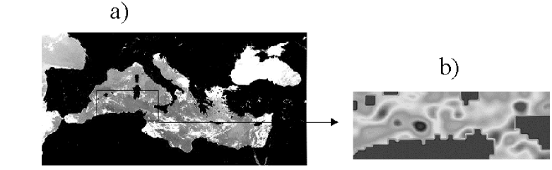
FIG. 1.: a) A map of the Mediterranean Sea. In the small box we show the area under study. b) Shows one of the altimetry images obtained from the satellite.

FIG. 2.: Linear-log plot of the fraction of variance of the eigenvalues in terms of their index.

FIG. 3.: Temporal modes associated the first two eigenvalues. Circles are the data for the first and squares for the second.

FIG. 4.: Power spectrum of the first four temporal modes. Circles, first mode; squares, second mode; triangles, third mode; and diamonds, fourth mode.

FIG. 5.: Linear-log plot showing the fraction of variance contained in the different eigenvalues starting from the third one.

FIG. 6.: Temporal modes for the third and fourth eigenfunctions. Squares, third mode; circles, fourth mode.

FIG. 7.: Temporal evolution of the third and fourth temporal modes obtained by numerical integration Eq. 19

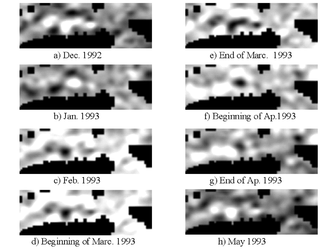
FIG. 8.: Numerical reconstruction of vortex shedding and motion near the Algerian coast. After h) the same sequence is repeated. The lighter area (higher altimetric values) next to the coast corresponds to an anticyclonic vortex (the moving coherent structure under study). In the figure, it always appears with its corresponding cyclonic vortex (darker area).

REFERENCES

- [1] P. Holmes, J.L. Lumley and G. Berkooz, Turbulence, Coherent Structures, Dynamical Systems and Symmetry, Cambridge University Press, Cambridge, 1996; P. Holmes, J.L. Lumley, G. Berkooz, J.C. Mattingly, and R.W. Wittenberg, Phys. Rep. 287 (1997), 337; G. Berkooz, P. Holmes, and J.L. Lumley, Annu. Rev. Fluid Mech. 25 (1993), 539.
- [2] J.L. Lumley, Stochastic Tools in Turbulence . Academic Press, New York, 1971.
- [3] R. W. Preisendorfer, Principal Component Analysis in Meteorology and Oceanography. Elsevier, Amsterdam, 1988.
- [4] A. Palacios, D. Armbruster, E.J. Kostelich, and E. Stone, Physica D 96 (1996), 132.
- [5] F. Qin, E.E. Wolf, and H.-C. Chang, Phys. Rev. Lett. 72 (1994), 1459.
- [6] C. López, A. Álvarez, and E. Hernández-García, Phys. Rev. Lett. 85 (2000), 2300.
- [7] A. Álvarez, C. López, M. Riera, E. Hernández-García, J. Tintoré, Geophys. Res. Lett. 27 (2000), 2709.
- [8] L. Sirovich and J.D. Rodríguez, Phys. Lett. A 120 (1987), 211.
- [9] L. Sirovich, Physica D 37 (1989), 126.
- [10] J.D. Rodríguez and L. Sirovich, Physica D 43 (1990), 77.
- [11] A.E. Deane, I.G. Kevrekidis, G.E. Karniadakis, and S.A. Orszag, Phys. Fluids A 3 (1991), 2337.
- [12] R.A. Sahan, A. Liakopoulos, H. Gunes, Phys. Fluids 9 (1997), 551.
- [13] N. Aubry, P. Holmes, J.L. Lumley, E. Stone, J. Fluid Mech. 192 (1988), 115.
- [14] N. Aubry, P. Holmes, J.L. Lumley, E. Stone, Physica D 37 (1989), 1.
- [15] M. Ghil, Dynamic Meteorology: Data Assimilation Methods, Springer-Verlag, New York, 1981.
- [16] K. Hasselmann, J. Geophys. Res. 93 (1988), 11015.
- [17] C. Uhl, R. Friedrich, and H. Haken, Phys. Rev. E 51 (1995), 3890.
- [18] F. Kwasniok, Phys. Rev. E 55 (1997), 5365.
- [19] U. Achatz, G. Schmitz, and K.-M. Greisiger, J. Atmos. Sci. 52 (1995), 3201.
- [20] F. Kwasniok, Physica D 92 (1996), 28.
- [21] See the different numbers of the AVISO Newsletter, available on-line at http://sirius-ci.cst.cnes.fr:8090/HTML/information/general/welcome.html.
- [22] The MSLA products are supplied by the CLS Space Oceanography Division (France), with financial support from the CEO programme (Center for Earth Observation) and Midi-Pyrénées regional council. CD ROMs are produced by the AVISO/Altimetry operations center. The ERS products were generated as part of the proposal Joint analysis of ERS-1, ERS-2 and TOPEX/POSEIDON altimeter data for oceanic circulation studies selected in response to the Announcement of Opportunity for ERS-1/2 by the European Space Agency (Proposal code: A02.F105); P. Y. Le Traon, J. Stum, J. Dorandeu, P. Gaspar and P. Vincent, J. Geophys. Res. 99 (1994), 24619; P. Y. Le Traon and F. Ogor, J. Geophys. Res. 103 (1998), 8045.
- [23] U. End, J. Font, G. Kraichman, C. Millot, M. Rhein and J. Tintoré, Prog. in Oceanog. 44 (1999), 37.
- [24] C. Bouzinac, J. Vazquez and J. Font, J. Geophys. Res. 103 (1998), 8059.
- [25] G. R. North, T. L. Bell, R. R. Cahalan and F.J. Moeng, Mon. Wea. Rev. 110 (1982), 699.
- [26] C. Bouzinac, PhD. Thesis, U. Pierre et Marie Curie, Paris, 1997.
- [27] F. P. Bretherton and M. Karweit, Mid-ocean mesoscale modeling in Modeling of transient or intermediate scale phenomena, National Academy of Science (1983), 237.
- [28] J. Pedlosky, Geophysical Fluid Dynamics (2nd edition). Springer-Verlag, New York, 1987.
- [29] M. Lesieur, Turbulence in Fluids. Kluwer, Dordretch, 1990.
- [30] B. Cushman-Roisin, Introduction to Geophysical Fluid Dynamics. Prentice-Hall, New Jersey, 1994.
- [31] J. Guckenheimer, A. Back, J. Guckenheimer, M. Myers, F. Wicklin and P. Worfolk, dstool: Computer Assisted Exploration of Dynamical Systems, Notices of the American Mathematical Society, 39 (1992), 303.